MSAE3111 Thermodynamics
Thermodynamics
Quiz 1
Includes only the Quiz 1 section.
States and Equation of States
Surrounding: usually used when describing heat flow from the surrounding to the system. Often referred to reservoir as well.
Extensive Properties: properties that are dependent on mass/volume/mole. (For example, momentum, energy, etc.)
Intensive Properties: properties that are independent on mass/volume/mole. (For example, energy per mole)
Quasi-static Changes: changes that are so slow such that you can assume certain variables/states being constant.
Reversible Processes:
processes whose entropy does not change, and therefore direction can be reversed/
they are usually very slow, because to avoid heat-generating work such as friction, which is related to the rate at which movement happens, we can minimize friction by simply moving really REALLY slowly.
- Volume Expansivity
- at constant pressure:
- at constant temperature:
- coefficient of linear expansion:
- Volume Expansion for system with $U(V,T,P)=U(P,T) \to V(P,T)$
- basically an equation of state defining a surface
-
Calculus Equations for $f(x,y,z)=0$ $$ {align} \begin{align} \left.\frac{\partial x}{\partial y}\right|_z &= \frac{1}{\left.\frac{\partial y}{\partial z}\right|_z}
\left.\frac{\partial x}{\partial y}\right|_z &= -\frac{\left.\frac{\partial x}{\partial z}\right|_y}{\left.\frac{\partial y}{\partial z}\right|_x}
\left.\frac{\partial x}{\partial y}\right|_z\left.\frac{\partial y}{\partial z}\right|_x\left.\frac{\partial z}{\partial x}\right|_y&=-1 \end{align*}$$
-
Volume Expansion for ideal gas
- realize they are not constants
-
Exact Differential
- basically, the function should not depend on path
So if: $$
dz=M(x,y)dx+N(x,y)dy\,\,\&\,\,\frac{\partial M}{\partial y}=\frac{\partial N}{\partial x}
$$ then $z$ is an exact differential, only dependent on the state $x,y$.
Work
-
Inexact Differential of Work Done for chemical system
- since work done is $W=\int_C \vec{F} \cdot d\vec{r}$, it is path dependent.
Positive Work Done: this is defined to be work done by the system (e.g. gas)
Negative Work Done: this is defined to be work done on the system (e.g. gas)
-
Inexact Differential of (Configurational) Work Done
-
wire/tension $$
d’W=-F_T dL
$$
-
magnetic dipole $$
d’W=-HdM
$$
-
electric dipole $$
d’W = -Ed\mathbb{P}
$$
-
surface film $$
d’W = -\sigma dA
$$
-
electrical cell $$
d’W=-\epsilon dz,\,\,\,\,z=charge
$$
where:
- there could be other dissipative/non-conservative work done for each system, but they are not listed here
-
First Law of Thermodynamics
- First Law of Thermodynamics:
- the work done through any adiabatic ($dQ=0$) path between two states are the same
- or generally:
$$
d’Q = dU + d’W
\[ where: obviously $U$ is a state function, independent of path. 4. ***Enthalpy for a Chemical System*** - given for a system, $d'W=PdV$, we can arrive at:\] d'Q |_P = d(U+PV)\equiv dH
$$
where:
- $H\equiv U+PV$ is enthalpy
-
Heat Capacity:
- how much heat to raise the temperature of a system of a given size:
which is path dependent since $Q$ is path dependent, and we define:
- at constant pressure:
-
at constant volume: $$
C_V \to Q V = \int{T_1}^{T_2}C_V dV $$
-
Heat Capacity for a Chemical System at a Constant Volume
- Since $d’Q = dU+PdV$, at constant volume:
-
Heat Capacity for a Chemical System at a Constant Pressure
-
Since $d’Q = dH - VdP$, at constant pressure: $$
\left.\frac{\partial’ Q}{\partial T}\right _P = \left. \frac{\partial H}{\partial T}\right _P = C_P $$
-
Internal Energy
-
Heat Equation with Specific Heat Capacities for Chemical System
-
From equation of $d’Q$ and $dU$, we get: $$
d’q = c_v dT+(\frac{c_P-c_v}{\beta v})dv
$$ where both $q$ and $v$ are normalized quantities from mole
-
-
Joule’s Coefficient:
-
it is a measured quantity with the following definition: $$
\left.\frac{\partial T}{\partial V}\right _U = \eta $$
where:
- for an ideal gas, this is $0$
-
- Free Expansion of Ideal Gas in Adiabatic Process
- Free expansion is different from adiabatic process, in which free expansion basically has $0$ external pressure $=$ $0$ pressure overall.
- Therefore, Free expansion means $d’W = 0$.
- Since we also have an adiabatic process, $d’Q = 0$.
- Therefore, we have $dU = 0$, so $dT = \Delta T = 0$
-
Coefficient of Free Expansion:
-
a measure of how a the internal energy of a free gas (expanding or compressing) changes at constant temperature.
-
this is derived quantity form the above using the relation $\left.\frac{\partial U}{\partial V}\right\vert _T\left.\frac{\partial V}{\partial T}\right\vert _U\left.\frac{\partial T}{\partial U}\right\vert _V = -1$ $$
\left. \frac{\partial U}{\partial V} \right _T \equiv FreeExpansion = -\eta C_V $$
where:
- for ideal gas, this quantity is $0$ since $\eta$ is 0.
-
-
Specific Heat Capacities and Coefficient of Free Expansion for Chemical System
- basically inserting the above into the equation $c_P - c_v = (\left.\frac{\partial U}{\partial V}\right\vert _T + P)\left. \frac{\partial V}{\partial T} \right\vert _P$
-
Specific Heat Capacities for Ideal Gas
-
basically knowing $\eta$ and $\left. \frac{\partial V}{\partial T} \right\vert _P$: $$
c_P - c_v = R
$$
-
-
Internal Energy Differential with Specific Heats
-
using equation (11), we have: $$
dU = C_V dT - \eta C_V dV
$$
-
-
Internal Energy with Specific Heats for Ideal Gas
-
because $\eta=0$ for ideal gas: $$
dU = C_V dT
U(T)=U(0)+\int_{T_0}^{T}C_V dT’$$
-
Enthalpy
- Joule-Thompson Experiment: Throttling of Gas
- basically, it is an adiabatic process where gas is transported from one chamber to another, such that:
or cleanly: $$
H_1 = H_2
\[ which is true in this case because ***throttling kept pressure to be constant/isobaric throughout the process*** 17. ***Joule-Thompson Experiment of Change of Temperature of a Gas*** - this a measured quantity, defining:\] \mu = \left. \frac{\partial T}{\partial P} \right|_h,\,\,\,\,where\,h=\frac{H}{moles}
$$
where:
- for **ideal gas,** $\mu=0$.
-
Specific Heat Capacity with Joule-Thompson Coefficient above
- basically, using the calculus result and cycle $\left. \frac{\partial h}{\partial T} \right\vert _P \left. \frac{\partial P}{\partial T} \right\vert _h\left. \frac{\partial T}{\partial h} \right\vert _P = -1$, we get
-
Specific Heat Capacities and Coefficient of Free Expansion for Chemical System
-
basically the other version of equation (12), using the result equation (18): $$
c_P - c_v = (\mu c_p+V)\left. \frac{\partial P}{\partial T} \right _V $$
-
-
Enthalpy and the Specific Heats
- since we knew $H(U,P,V)=H(P,V)$, we can also say $H(T,P)$
-
Enthalpy and the Specific Heats for Ideal Gas
-
Using the relation $\mu = 0$ for ideal gas, and the equation (20), we know: $$
dh=c_p dT
h(T) = h(T_0) + \int_{T_0}^{T} c_p dT’$$
-
-
Heat Capacities for an Reversible Process with Ideal Gas
- if we have an reversible process ($dS=0$), it has to be also adiabatic (since $d’Q = TdS$). Then using the two equations their their differential version of it, we get using equation (15) and (20) with ideal gas condition:
Hence, by dividing the above two equations we can arrive at: $$
\frac{c_v dT}{c_p dT} = -\frac{Pdv}{vdP}
\frac{c_v}{c_p} = -\frac{Pdv}{vdP}
\frac{dP}{P} = -\frac{c_p}{c_v}\frac{dv}{v}
ln(PV^\gamma) = constant
PV^\gamma = constant
  \gamma = \frac{c_p}{c_v} > 1


  $$
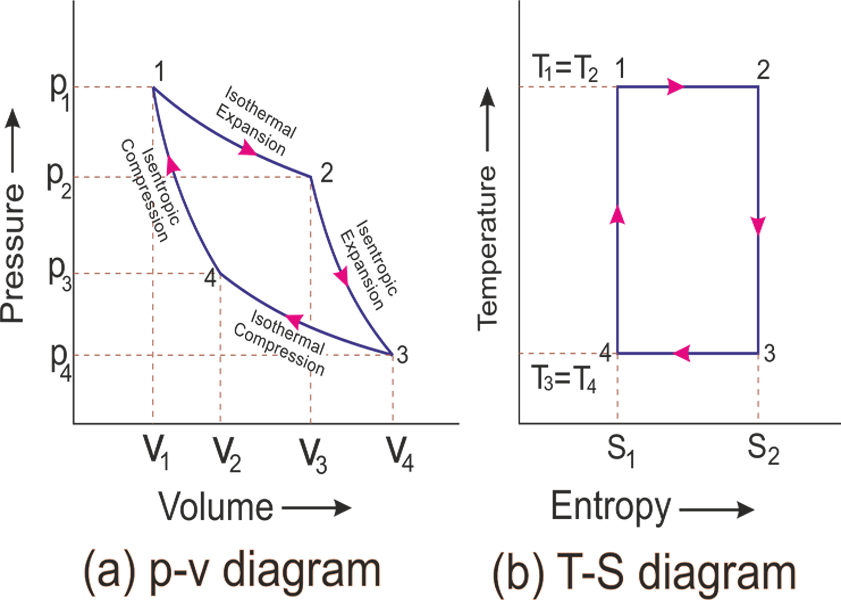
Carnot Cycle
For this section, refer to this diagram (again, ideal gas is assumed):

-
Carnot Cycle Heat Quotient
-
Consider the process 1 and process 3, we can compute the ratio of the heat: $$
\[now, since we know process 2 and process 4 are adiabatic processes, using equation (22), we found:\]\frac{Q_1}{ Q_3 }=\frac{T_1ln(\frac{V_2}{V_1})}{T_3 ln(\frac{V_3}{V_4})} T_2V_2^{\gamma}=T_1V_2^{\gamma}=T_3V_3^{\gamma}
\[dividing the above two, we obtain:\]
T_4V_4^{\gamma}=T_3V_4^{\gamma}=T_1V_1^{\gamma}\\frac{T_1V_2^{\gamma}}{T_1V_1^{\gamma}}=\frac{T_3V_3^{\gamma}}{T_3V_4^{\gamma}}
\[Hence the above equation reduces to:\]
\frac{V_2^{\gamma}}{V_1^{\gamma}}=\frac{V_3^{\gamma}}{V_4^{\gamma}}
\frac{V_2}{V_1}=\frac{V_3}{V_4}\frac{Q_1}{ Q_3 }=\frac{T_1}{T_3} $$
-
Thermal Efficiency: This is defined to be the ratio of total work done over total heat input $$
\eta = \frac{W}{Q_{in}}
$$
-
Carnot Cycle Work Done
-
for processes 2 and process 4, we knew that $Q=0$ since they are adiabatic.
-
the total work done for both processes is therefore: $$
0-\Delta U=\Delta W
\[but as for ideal gas, $U=U(T,C_{V_{(T)}})$, hence as the net change in temperature is 0:\]0=\Delta W
$$
-
-
Thermal Efficiency for Carnot Engines
-
using the equation (24) and the above fact for thermal efficiency, we obtain, for a carnot cycle/engine: $$
\eta = \frac{Q_1 + Q_3}{Q_1}= \frac{Q_1 - |Q_3|}{Q_1}
\eta = 1-\frac{T_3}{T_1}$$ where:
- $T_1$ is the higher temperature in the graph.
-
- Reverse Carnot Cycle for a Refrigerator:
- Basically we will have heat flowing in process 3 at room temperature, and heat flowing out in process 1. (Therefore, reversing the cycle.)
- Now, we can reach the same formula for net work done/heat flow, but with a negative sign, indicating that work done is needed on the system.
Figure of Merit: This is the refrigerator version for thermal efficiency, we take the ratio of heat removed/taken in over work done onto/supplied to the system. $$
c=\frac{Q_{in}}{ W } $$
- we took $\vert W\vert$ because work done would be negative.
Entropy
This explains why not all processes are reversible, even if energetically permittable.
In some of the equations below, this graph will still be used:
Second law of Thermodynamics:
- every process in an isolated entity (including the universe, if is acted on/by) can either have entropy $S$ staying the same or increase.
- $\to$ in a reversible process, entropy $S$ must stay the same
- $\to$ there is no perfect heat engine/refrigerator
-
Closed Loops in Carnot Cycle with Ideal Gas
-
for the closed loop in the figure above. and using equation (24), we know: $$
\frac{Q_1}{-Q_3}=\frac{T_1}{T_3}
\[since the other two processes are adiabatic, we know:\]
\frac{Q_1}{T_1}+\frac{Q_3}{T_3}=0\sum_i \frac{Q_i}{T_i} =0
\[Now, if we take infinitesimal loops, such that the two isothermal curve approach each other:\]\sum_i \frac{Q_i}{T_i} = \sum_i \frac{Q_1 - |Q_3|}{T_i} \approx \sum_i \frac{d’Q}{T_i}=0
\[However, since the above is an infinitesimal loop on the $P-V$ plane, we can construct any over loop by adding those small loops: - notice that this also makes the conclusion general to other **non-ideal gases** as well\]
\oint_{carnot}\frac{d’Q}{T}=0\oint_{P-V\,plane}\frac{d’Q}{T}=0
$$
-
-
Entropy
-
from the above, we can define the quantity entropy with an heat flow in a reversible process (since derived in Carnot Cycle) to be: $$
dS \equiv \frac{d’Q_{rev}}{T}\,\,or\,\,d’Q_{rev} = TdS
\[Therefore, we obtain the ***general result for any gas in the $P-V$ plane***:\]\oint_{P-V\,plane}\frac{d’Q}{T}=\oint_{P-V\,plane} dS = 0
$$
-
-
State of $S$
-
notice that equation (27) effectively made entropy $S$ become independent of path in the $P-V$ plane. Therefore, we conclude that: $$
S=S(P,V)
$$
-
now, if we use it for ideal gas, we get: $$
S=S(P,V)=S(P,T)=S(T,V)
$$
-
-
First law of Thermodynamics Combined with Entropy for Chemical Systems
-
using equation (27), we can write (if we have a reversible process): $$
d’Q =dU+d’W
TdS=dU+PdV$$
-
-
Specific Heats with Entropy
-
basically we have an alternative expression of $d’Q$, so we can express many things alternatively: $$
C_V = \left. \frac{d’Q}{dT} \right _V = T\left. \frac{dS}{dT} \right _V \ C_P = \left. \frac{d’Q}{dT} \right _P = T\left. \frac{dS}{dT} \right _P $$ and etc.
-
-
Carnot Cycle in $T-S$ Plane
-
since Carnot cycle basically contains isothermal and adiabatic processes, we can construct the same cycle in the diagram below:
-
Midterm
Includes this section and cumulatively, all the previous sections.
Entropy and Ideal Gas
-
Entropy Differentials for Ideal Gas
Since we know, for ideal gas, $dU = C_V dT - \eta C_V dV = C_V dT$, and $TdS = dU + PdV$ for a system: $$
TdS = C_V dT + PdV
\[since:\]
dS = \frac{C_V}{T}dT + \frac{P}{T}dV
\[we arrive at:\]dS = \left.\frac{\partial S}{\partial T}\right _V dT + \left.\frac{\partial S}{\partial V}\right _TdV \begin{cases} \text{for ideal gas:} & \left.\frac{\partial S}{\partial T}\right|_V = \frac{C_V}{T}
& \left.\frac{\partial S}{\partial V}\right|_T = \frac{P}{T}=\frac{nR}{V}
\text{in general:} & \left.\frac{\partial S}{\partial T}\right|_V = \frac{C_V}{T}
& \left.\frac{\partial S}{\partial V}\right|_T = \frac{P}{T}-\eta \frac{C_V}{T} \end{cases}$$
-
Entropy Integral for Ideal Gas
Using the above, we could explicitly calculate the change of entropy for an ideal gas: $$
dS = C_V \frac{dT}{T} + nR \frac{dV}{V}
\[so:\]S_2 - S_1 = C_V ln(\frac{T_2}{T_1}) + nRln(\frac{V_2}{V_1})
$$
Heat/Entropy Change for Reversible Process
Now we are dealing with processes, so the second law of thermodynamics takes precedence.
- if we are just dealing with a state of a system, use the first law.
If we have a reversible process, we could also use the relation $d’Q = TdS$.
-
Change of Entropy for Reversible Isothermal Process
Again, since it is isothermal and reversible, we can use $d’Q = TdS$: $$
S_2 - S_1 = \int_{Q_a}^{Q_b} \frac{d’Q}{T}=\frac{1}{T}(Q_b - Q_a)
$$ which means, at the constant temperature:
- net heat flow in = increase in entropy
- net heat flow out = decrease in entropy = not possible to happen
-
Change of Entropy for Reversible Isochoric Process
In addition to using $d’Q = TdS$, we also know $d’Q\vert _V = dU\vert _V = C_V dT + 0$
So we have: $$
S_2 - S_1 = \int_{T_a}^{T_b} C_V\frac{ dT}{T}=C_V ln(\frac{T_b}{T_a}),\,\,\text{if $C_V$ is independent of $T$}
$$
-
Change of Entropy for Reversible Isobaric Process
Now, we use the equation $d’Q\vert _P = dH\vert _P = C_p dT - \mu C_p dP = C_p dT$
Therefore we have: $$
S_2 - S_1 = \int_{T_a}^{T_b} C_P\frac{ dT}{T}=C_P ln(\frac{T_b}{T_a}),\,\,\text{if $C_P$ is independent of $T$}
$$
-
Reversible Heat Flow:
In all the last two cases above, we have $\Delta S$ dependent on change of $T$. This implies that, in order for a reversible process and a reversible heat flow to occur, we need to raise the temperature of the system as a sequence of infinitesimal steps $\delta T$:
$$
\begin{cases}
dS_{system} = C_{P\,or\,V} \frac{\delta T}{T}
dS_{surronding} = C_{P\,or\,V} \frac{\delta T}{T+2\delta T} \approx C_{P\,or\,V} \frac{\delta T}{T}
\end{cases}
dS_{system} + dS_{surronding} = 0
\[which is **reversible heat flow**. ### Heat/Entropy Change for Irreversible Process The **key idea/trick** is that: - for each **step**/change, you can compute it using the **reversible process** as **$S$ is a state equation** - this means, for each **change of the system or the surrounding *individually***, you can use reversible process calculation - then, a **process basically involves the sum of changes of each part of the system** (including surrounding) - you will find the **total change of $S$ will be non-zero** 35. ***Change of Entropy at Either Constant P/V in an Irreversible Process*** The idea is as follows <img src="\lectures\images\typora-user-images\image-20201013171252696.png" alt="image-20201013171252696" style="zoom:67%;" /> and we treat the ***system individually*** first, **going from state $T_1 \to T_2$:**\]\Delta S_{sys} = C_{P\,or\,V} \cdot ln(\frac{T_2}{T_1})
$$
where:
- this is legal to treat it as reversible process, **because for a system, it is merely a change of state, which is independent of path.**
now, treat the ***surrounding individually***, going from $T_2 \to T_2$, but with a heat flow known:
$$
\begin{align*}
\Delta S_{surr} &= \frac{1}{T}\int_{Q_a}^{Q_b} d'Q \\
&= \frac{1}{T_2}(-\Delta Q_{sys}) \\
&= \frac{1}{T_2}\left(- \int_{T_1}^{T_2}C_{P\,or\,V} \cdot dT\right)\\
&= -\frac{1}{T_2}C_{P \, or\,V}\left(T_2 - T_1\right)
\end{align*}
$$
Therefore, the **total change for the process becomes**:
$$
\begin{align*}
\Delta S_{total} &= \Delta S_{sys}+ \Delta S_{surr} \\
\Delta S_{total} &= C_{P\,or\,V} \cdot ln\left(\frac{T_2}{T_1}\right) - C_{P \, or\,V}\frac{\left(T_2 - T_1\right)}{T_2}
\end{align*}
$$
-
Second Law of Thermodynamics
If we convert the previous equation (35) into the form: $$
\Delta S_{total} = C_{P \,or\,V} \left( ln(1+x)-1+\frac{1}{1+x} \right)
\[where: - $x = \frac{T_2 - T_1}{T_1}$ It can be plotted to show that:\]\Delta S {total} = \Delta S{universe} \ge 0
$$
Energy Degradation
This is to show that, if you have done irreversible process/increased entropy, then the ability of doing work is reduced
- i.e. the maximum efficiency will go down
-
Work Lost Due to Irreversible Process/Increase in Entropy
Consider the same process, reached via two different path:

where:
- dotted lines indicate a reversible process
- solid line indicates an irreversible process
Path (a): $$
W_{max} = \eta Q_{in} = Q_{in}\left(1-\frac{T_0}{T_1}\right)
\[Path (b):\]W_{max} = \eta Q_{in} = Q_{in}\left(1-\frac{T_0}{T_2}\right)
\[Now, if $T_2 > T_1$, we see that the maximum work is different. Consider the **irreversible step** in path (a):\]\begin{align} \Delta S &= \Delta S_1 + \Delta S_2
\[where: - obviously we assumed the reservoir to be large enough so its temperature stayed constant - also, $T_2 > T_1$ complies to our assumption Lastly, we see that:\]
&= \frac{Q}{T_1}+\frac{-Q}{T_2}
&= Q\left(\frac{1}{T_1}-\frac{1}{T_2}\right) \end{align}\begin{align} W_{lost} &= Q_{in}\left(1-\frac{T_0}{T_2}\right) - Q_{in}\left(1-\frac{T_0}{T_1}\right)
&= T_0 Q_{in} \left( \frac{1}{T_1}-\frac{1}{T_2} \right)
&= \frac{Q_{in}}{Q}T_0\Delta S_{total} \end{align}$$ where:
- $Q$ is irreversible heat
- $Q_{in}$ is reversible heat
-
Work Lost and Entropy
If we make $Q_{in} = Q$, namely all the heat into the system is irreversible:
- we can do this as $Q$ was an arbitrary quantity
Gas Mixing Contradiction
-
Ideal Gas Mixing during an Adiabatic Free Expansion
If we have an adiabatic process, it means $d’Q = 0$. A free expansion means no external pressure, hence $d’W=0$.
- therefore, we conclude that $dU=0$, so $T$ of gas has to stay constant.

Then we have: $$
\Delta S_{He} = \Delta S_{Ne},\,\,\text{assuming their $C_{V,P}$ are also the same}
\[hence:\]\Delta S_{total} = 2\Delta S_{He} = 2\left( nRln\left( \frac{2V_1}{V_1} \right) \right) = 2nRln(2)
\[However, if we simply change the $Ne$ to $He$, we would have a homogenous mixing, then it must be:\]\Delta S_{total}=0
\[since **homogenous mixing must be reversible**. And the solution is that we need to fix our equation of $\Delta S$ to include:\]\Delta S = C_V ln\left( \frac{T_2}{T_1} \right) + nR ln\left( \frac{M_2}{M_1} \right)
$$ where:
- $M=\frac{1}{concentration}$, instead of having volume inside.
Thermodynamic Processes
-
Thermodynamic Processes of a Large Reservoir
If you have a large reservoir of temperature $T_{res}$, and $Q$ is the heat flows into the system from it, then from the second law of thermodynamics: $$
\begin{align} \Delta S_{uni} &\ge 0
\Delta S_{sys} + \Delta S_{res} &\ge 0
\Delta S_{sys} + \frac{-Q}{T_{res}} &\ge 0
T_{res}\Delta S_{sys} &\ge Q
T_{res}\Delta S_{sys} &\ge \Delta U_{sys} + P_{sys}\Delta V_{sys}
\end{align}$$ for any process.
-
Thermodynamic Processes of a Large Reservoir using Enthalpy
Same as the above setting (41), but we use $d’Q = dH - VdP$: $$
T_{res}\Delta S_{sys} \ge \Delta H_{sys} - V_{sys}\Delta P_{sys}
$$
List of Useful Theorems
Thermodynamics
Theorem
By definition, $\left.\frac{\partial U}{\partial T}\right\vert _{V}=V\beta$ , $\left.\frac{\partial U}{\partial T}\right\vert _{P}=-V\kappa_T$ $$
dU=\beta VdT-\kappa_T V dP
$$
Statistical Mechanics
Kinetic Theory
Equation Appendix
| Equation Number | Title/Condition | Equations | |
|---|---|---|---|
| 1 | chemical system | \(dV=\beta V dT - \kappa_T VdP\) | |
| 2 | chemical system | \(d'W= \vec{F} \cdot d \vec{r} = PAdx=PdV\) | |
| 3 | First Law of Thermodynamics | $d’Q = dU + d’W$ | |
| chemical system | $d’Q = dU + PdV$ | ||
| chemical system | $d’Q = dH - VdP$ | ||
| 4 | chemical system | $H\equiv U+PV$ | |
| 5 | wire/tension | \(d'W=-F_T dL\) | |
| magnetic dipole | $d’W=-HdM$ | ||
| electric dipole | $d’W = -Ed\mathbb{P}$ | ||
| surface film | $d’W = -\sigma dA$ | ||
| electrical cell | $d’W=-\epsilon dz,\,\,\,\,z=charge$ | ||
| 6 | $\left.\frac{\partial’ Q}{\partial T}\right\vert _V= \left. \frac{\partial U}{\partial T}\right\vert _V = C_V$ | ||
| 7 | $\left.\frac{\partial’ Q}{\partial T}\right\vert _P= \left. \frac{\partial H}{\partial T}\right\vert _P = C_P$ | ||
| 8 | Volumetric Expansion Coefficient | $$\beta = \frac{1}{V}\left.\frac{\partial V}{\partial T}\right | _P$$ |
| $$\kappa_T = -\frac{1}{V}\left.\frac{\partial V}{\partial P}\right | _T$$ | ||
| \(\alpha = \frac{1}{3}\beta\) | |||
| 9 | chemical system | $d’q = c_v dT+(\frac{c_P-c_v}{\beta v})dv$ | |
| 10 | chemical system | $\left.\frac{\partial T}{\partial V}\right\vert _U = \eta$ | |
| 11 | Coefficient of Free Expansion | $\left. \frac{\partial U}{\partial V} \right\vert _T\equiv -\eta C_V$ | |
| 12 | chemical system | $$c_P - c_v = (P-\eta c_V)\left. \frac{\partial V}{\partial T} \right | _P$$ |
| 13 | ideal gas | $c_P - c_v = R$ | |
| 14 | $dU = C_V dT - \eta C_V dV$ | ||
| 15 | $dU = C_V dT$ | ||
| analogy to (21): $U(T)=U(0)+\int_{T_0}^{T}C_V dT’$ | |||
| 16 | Chemical, isobaric processes: | $U_2+P_2V_2 = P_1V_1+ U_1$ | |
| $H_2 = H_1$ | |||
| 17 | $\mu = \left. \frac{\partial T}{\partial P} \right\vert _h,\,\,\,\,where\,h=\frac{H}{moles}$ | ||
| 18 | $\left. \frac{\partial h}{\partial P} \right\vert _T = -\,u c_p$ | ||
| 19 | chemical system | $c_P - c_v = (\mu c_p+V)\left. \frac{\partial P}{\partial T} \right\vert _V$ | |
| 20 | $dh= \left. \frac{\partial h}{\partial T}\right\vert _P dT+\left. \frac{\partial h}{\partial P}\right\vert _T dP$ | ||
| $dh = c_p dT - \mu c_p dP$ | |||
| 21 | $dh=c_p dT$ | ||
| analogy to (15): $h(T) = h(T_0) + \int_{T_0}^{T} c_p dT’$ | |||
| 22 | ideal gas, adiabatic process | $\gamma = \frac{c_p}{c_v} > 1$ | |
| 23 | ideal gas, adiabatic process | $PV^\gamma = constant$, for \(\gamma = \frac{c_p}{c_v} > 1\) | |
| ideal gas, isothermal process | $PV= constant=nRT_0$ | ||
| 24 | in a Carnot cycle, two isothermal processes | $\frac{Q_1}{\vert Q_3\vert }=\frac{T_1}{T_3}$ | |
| 25 | ideal thermal efficiency for Carnot engine | $\eta = 1-\frac{T_3}{T_1}$ | |
| 26 | for any gas | $\oint_{P-V\,plane}\frac{dQ}{T}=0$ | |
| 27 | In a reversible process | $d’Q = TdS$ | |
| for any gas: $\oint_{P-V\,plane} dS = 0$ | |||
| 28 | chemical system, reversible process | $TdS=dU+PdV$ | |
| 29 | for ideal gas | $\left.\frac{\partial S}{\partial T}\right\vert _V = \frac{C_V}{T}$ | |
| for ideal gas | $\left.\frac{\partial S}{\partial V}\right\vert _T = \frac{P}{T}=\frac{nR}{V}$ | ||
| for chemical system | $\left.\frac{\partial S}{\partial T}\right\vert _V = \frac{C_V}{T}$ | ||
| for chemical system | $\left.\frac{\partial S}{\partial V}\right\vert _T = \frac{P}{T}-\eta \frac{C_V}{T}$ | ||
| 30 | for ideal gas | $S_2 - S_1 = C_V ln(\frac{T_2}{T_1}) + nRln(\frac{V_2}{V_1})$ | |
| 31 | isothermal reversible process | $S_2 - S_1 = \int_{Q_a}^{Q_b} \frac{d’Q}{T}=\frac{1}{T}(Q_b - Q_a)$ | |
| 32 | isobaric reversible process | $S_2 - S_1 =C_V ln(\frac{T_b}{T_a}),\,\,\text{if$C_V$is independent of$T$}$ | |
| 33 | isobaric reversible process | $S_2 - S_1 =C_P ln(\frac{T_b}{T_a}),\,\,\text{if$C_P$is independent of$T$}$ | |
| 34 | reversible heat flow requires a sequence of infinitesimal heat transaction of $\delta T$ | ||
| 35 | for a chemical system | $\Delta S_{total} = \Delta S_{sys}+ \Delta S_{surr}= C_{P\,or\,V} \cdot ln\left(\frac{T_2}{T_1}\right) - C_{P \, or\,V}\frac{\left(T_2 - T_1\right)}{T_2}$ | |
| 36 | Second Law of Thermodynamics | $\Delta S {total} = \Delta S{universe} \ge 0$ | |
| 37 | Irreversible heat transfer between two large reservoir | $\Delta S = Q\left(\frac{1}{T_1}-\frac{1}{T_2}\right),\,\,\text{where$T_2 > T_1$}$ | |
| 38 | for $Q$ being heat transfer (37) in irreversible process | $W_{lost}=\frac{Q_{in}}{Q}T_{sys}\Delta S_{universe}$ | |
| 39 | if $Q$ is the same as $Q_{in}$ to the system (38), or all $Q_{in}$ is irreversible | $W_{lost} = T_{sys} \Delta S_{universe}$ | |
| 40 | Lagrange Multiplier | $\vec{\nabla}f(x,y)=\lambda \vec{\nabla}g(x,y)$, $g(x,y)$ being the constraint | |
| one usage of this: nature prefers to maximize $S$ under certain constraint | |||
| 41 | Process with a large reservoir of $T_{res}$ | $T_{res}\Delta S_{sys} \ge \Delta U_{sys} + P\Delta V_{sys}$ | |
| 42 | Process with a large reservoir of $T_{res}$ | $T_{res}\Delta S_{sys} \ge \Delta H_{sys} - V_{sys}\Delta P_{sys}$ | |
| 43 | Helmholtz Energy (Third Potential) | $F=U-TS$ | |
| 44 | Gibbs Free Energy (Fourth Potential) | $G=U+PV-TS$ | |
| $G=F+PV$ | |||
| $G=H-TS$ | |||
| 45 | For a process | $dF \le W_{total}$ | |
| For $W_{total}=W_{PdV}+W_{non-PdV}$, $W_{non-PdV}=0$ | $dF\le 0$, at constant volume | ||
| 46 | For a process at constant $T,V$, no $W_{Non-PdV}$ | $dF \le 0$ | |
| For a process at constant $T,P$, no $W_{Non-PdV}$ | $dG \le 0$ | ||
| 47 | Second Law (Process) on First Potential | $dU_{sys} \le T_{res}dS_{sys}-d’W_{sys}$ | |
| Second Law (Process) on Second Potential | $dH_{sys} \le T_{res}dS_{sys}+V_{sys}dP_{sys}$ | ||
| Second Law (Process) on Third Potential | $dF_{sys} \le -S_{sys}dT_{res}-P_{sys}dV_{sys}$ | ||
| Second Law (Process) on Fourth Potential | $dG_{sys} \le -S_{sys}dT_{res}+V_{sys}dP_{sys}$ | ||
| 48 | First Potential Derivatives | $\left.\frac{\partial U}{\partial S}\right\vert _V = T$, $\left.\frac{\partial U}{\partial V}\right\vert _S = -P$ | |
| Second Potential Derivatives | $\left.\frac{\partial H}{\partial S}\right\vert _V = T$, $\left.\frac{\partial H}{\partial P}\right\vert _S = V$ | ||
| Third Potential Derivatives | $\left.\frac{\partial F}{\partial T}\right\vert _V = -S$, $\left.\frac{\partial F}{\partial V}\right\vert _T = -P$ | ||
| Fourth Potential Derivatives | $\left.\frac{\partial G}{\partial T}\right\vert _P = -S$, $\left.\frac{\partial G}{\partial P}\right\vert _T = V$ | ||
| 49 | Using (48) | $U=F-T\left.\frac{\partial F}{\partial T}\right\vert _V$ | |
| $H=F-T\left.\frac{\partial F}{\partial T}\right\vert _V-V\left.\frac{\partial F}{\partial V}\right\vert _T$ | |||
| $G=F-V\left.\frac{\partial F}{\partial V}\right\vert _T$ | |||
| 50 | $\left.\frac{\partial^2 G}{\partial T^2}\right\vert _P = -\frac{C_P}{T}$ | ||
| 51 | $\left.\frac{\partial^2 G}{\partial P^2}\right\vert _T = -\kappa_T V$ | ||
| 52 | $\left.\frac{\partial^2 G}{\partial T\partial P}\right\vert _T = \beta V$ | ||
| 53 | Maxwell’s Relations | $\left.\frac{\partial T}{\partial V}\right\vert _S = -\left.\frac{\partial P}{\partial S}\right\vert _V$ | |
| $\left.\frac{\partial T}{\partial P}\right\vert _S = \left.\frac{\partial V}{\partial S}\right\vert _P$ | |||
| $\left.\frac{\partial S}{\partial V}\right\vert _T = \left.\frac{\partial P}{\partial T}\right\vert _V$ | |||
| $\left.\frac{\partial S}{\partial P}\right\vert _T = -\left.\frac{\partial V}{\partial T}\right\vert _P$ | |||
| 54 | $TdS$ Equations | $TdS=C_V dT + T\left.\frac{\partial P}{\partial T}\right\vert _V dV$ | |
| $TdS=C_P dT - T\left.\frac{\partial V}{\partial T}\right\vert _P dP$ | |||
| $TdS=C_P \left.\frac{\partial T}{\partial V}\right\vert _PdV + C_V \left.\frac{\partial T}{\partial P}\right\vert _VdP$ | |||
| 55,56,57 | All derived from (54) | $\Delta S = \int\limits_{T_0}^T \frac{C_P}{T’}dT’-\int\limits_{P_0}^P \left.\frac{\partial V}{\partial T}\right\vert _P dP’$ | |
| $\Delta C_V\vert {T_0} = T_0\int\limits{V_0}^V \left.\frac{\partial^2 P}{\partial T^2}\right\vert _VdV$ | |||
| $\Delta C_P\vert {T_0} = T_0\int\limits{P_0}^P \left.\frac{\partial^2 V}{\partial T^2}\right\vert _P dV$ | |||
| $-\eta C_V=T\left.\frac{\partial P}{\partial T}\right\vert _V -P$ | |||
| 58 | For ideal gas, using (30) | $S_2 - S_1 = C_P ln(\frac{T_2}{T_1}) - nRln(\frac{P_2}{P_1})$ | |
| 59 | For ideal gas, using $G=H-TS$ | $G=nRT\left(ln(P)+\Phi(T)\right)$, $\Phi(T)$ is some function on $T$ only. | |
| 60 | For ideal gas reaction, at constant temperature using (59) | $G(P_f) = G(P_i) + nRTln(\frac{P_f}{P_i})$ |
| Equation Number | Title/Condition | Equations |
|---|---|---|
| 61 | For ideal gas reaction at constant temperature, | $aA+bB \to cC+dD$ |
| (derived using (60)) | $\frac{(P_C)^c(P_D)^d}{(P_A)^a(P_B)^b}=e^{-\frac{\Delta G^\circ}{RT}}\equiv k$ | |
| 62 | Chemical Potential | $\mu \equiv \left.\frac{\partial G}{\partial N}\right\vert _{T,P}$ |
| 63 | At constant pressure during phase transition | $\Delta H > \Delta U$, if $\Delta V >0$ |
| 64 | During phase transition | $\begin{cases}g_{s}=g_{l} & \text{at melting temperature}\ g_{l}=g_{g} &\text{at boiling temperature}\ g_{s}=g_{g} &\text{at sublimation temperature}\end{cases}$ |
| 65 | At phase transition (hence constant $T$) | $\begin{cases}l_{s\to l}=\text{heat of fusion}\ l_{l\to g}=\text{heat of vaporization}\ l_{s\to g}=\text{heat of sublimation}\end{cases}$ |
| Above is also $\Delta H$ at constant $P$ during phase change. | ||
| 66 | reversible process | $\begin{cases}\Delta S_{s\to l}=\frac{l_{s\to l}}{T}\ \Delta S_{l\to g}=\frac{l_{l\to g}}{T}\ \Delta S_{s\to g}=\frac{l_{s\to g}}{T}\end{cases}$ |
| 67 | At constant temperature and pressure | $\Delta G=0$ at phase transition |
| 68 | Clausius Chaperone Equation | $\left.\frac{\partial P}{\partial T}\right\vert {s,l\,eqilib}=\frac{l{s\to l}}{T_{melting}}\frac{1}{v_l - v_s}$ |
| In general: $\left.\frac{\partial P}{\partial T}\right\vert {phase\,eqilib}=\frac{l{phase\,trans}}{T_{phase\,trans}}\frac{1}{\Delta v_{phase}}$ | ||
| 69 | For ideal gas, at liquid gas boundary, assuming $v_g - v_l \approx v_g$ | $P=Ae^{\frac{-l_{l \to g}}{RT}}$ |
| $$ | ||
| 70 | Energy Density (Radiation) of a Black Body | $u=\sigma T^4$ |
| 71 | Other properties of a Black Body | $P=\frac{1}{3}\sigma T^4$ |
| $U=\sigma T^4V$ | ||
| $C_v = 4\sigma T^3V$ | ||
| $TdS=4\sigma VT^3 dT + \frac{4}{3}\sigma T^4 dV$ | ||
| 72 | Heat needed for a reversible, isothermal volume expansion of Black Body | $\Delta Q = \frac{4}{3} \sigma T^4\Delta V$ |
| 73 | Reversible adiabatic process of Black Body | $VT^3=constant$ |
| 90 | Third Law of Thermodynamics: | $T \to 0$ means $\Delta S \to 0$ (technically a constant) |
| $C_{p,v}\to 0$ as $T \to 0$ | ||
| $\beta \to 0$ as $T \to 0$ | ||
| 91 | Experimental Property of Black Body Radiation | $Radiation \propto Energy \,Density\, (\frac{U}{V}=u)$ |
| $u=u(T)$ only | ||
| Radiation Pressure: $P=\frac{u}{3}$ | ||
| 74 | Overall Principle of Statistical Mechanics | All microstates are equally probable |
| $S = k_B ln(\Omega)$, $\Omega = \text{number of microstates}$ | ||
| 75, 76 | Canonical Ensemble | $P(E_s) = \frac{e^{-\beta E_s}}{\sum e^{-\beta E_s}}$ or $P(E_s) = \frac{g_ie^{-\beta E_s}}{\sum g_ie^{-\beta E_s}}$ |
| (Canonical) Partition function | $z=\sum e^{-\beta E_s}$ | |
| $\beta = \frac{1}{k_BT}$ | ||
| $U = \langle E_{sys}\rangle = \sum E_s P(E_s)= \frac{\sum E_se^{-\beta E_s}}{\sum e^{-\beta E_s}}$ | ||
| 77 | Grand Canonical Ensemble | $P(E_s) = \frac{e^{-\beta E_s-\alpha N_s}}{\sum e^{-\beta E_s-\alpha N_s}}$ |
| Grand Canonical Partition function | $z=\sum e^{-\beta E_s-\alpha N_s}$ | |
| $U = \frac{\sum E_se^{-\beta E_s-\alpha N_s}}{\sum e^{-\beta E_s - \alpha N_s}}$ | ||
| $\langle N_{sys}\rangle = \frac{\sum N_se^{-\beta E_s-\alpha N_s}}{\sum e^{-\beta E_s - \alpha N_s}}$ | ||
| 78 | Macroscopic Property $Y$ of a Macrostate | $\langle Y \rangle =\frac{\sum Y_k w_k}{\sum w_k}$ |
| usually, $\sum w_k=1$ | ||
| 79 | Number of Microstates for System Without Degeneracy | $\Omega =\frac{N!}{\Pi_i (n_i)!}$ |
| (Microcanonical Ensemble) | for $\begin{cases}n_1&\text{$n_1$particles in energy state 1}\n_2&\text{$n_2$particles in energy state 2}\n_1&\text{$n_3$particles in energy state 3}\…\n_n&\text{$n_n$particles in energy state n}\end{cases}$ | |
| 80 | Number of Microstates for System With Degeneracy | $\Omega= \frac{N!}{\Pi_i \left(\frac{n_i}{g_i^{ni}}\right)!}$ |
| (Microcanonical Ensemble) | for $\begin{cases}g_1&\text{$g_1$degeneracy in energy state 1}\g_2&\text{$g_2$degeneracy in energy state 2}\g_1&\text{$g_3$degeneracy in energy state 3}\…\g_n&\text{$g_n$degeneracy in energy state n}\end{cases}$ | |
| 81 | Energy levels in Microcanonical Ensemble | $E_n \approx n\hbar \omega$ |
| $q \equiv \text{total level of excitation/ totoal # energy level}$ | ||
| 82 | Number of Microstates for System | $\Omega = \frac{(q+(N-1))!}{q!(N-1)!}\approx\frac{(q+N)!}{q!N!}$ |
| (Microcanonical Ensemble) | since $N \gg 1$ | |
| 83 | Stirling’s Approximation | $ln(n!)\approx nln(n)-n$ |
| 84 | Entropy of System given $q$ and $N$ | $S=k_Bln\left(\frac{(q+N)!}{q!N!}\right)$ |
| Using (83) | $S=k_B\left[ (q+N)ln(q+N)-qln(q)-Nln(N) \right]$ | |
| 85 | Energy for Microcanonical Ensemble using $T$ | $U=\frac{U_0}{e^{\frac{\hbar \omega}{k_B T}}-1}=\frac{N\hbar \omega}{e^{\frac{\hbar \omega}{k_B T}}-1}$ |
| For $\begin{cases}U_{sys} = U = q\hbar \omega \ U_0 := N\hbar \omega\end{cases}$ | ||
| 86 | Microcanonical Ensemble Average Energy per Oscillator | $U_{\text{per oscillator}}=\frac{\hbar \omega}{e^{\frac{\hbar \omega}{k_bB T}}-1}$ |
| \(q_{\text{per oscillator}}=\frac{1}{e^{\frac{\hbar \omega}{k_bB T}}-1}\) | ||
| 87 | Microcanonical Ensemble $C_V$ | $C_V=Nk_B\left(\frac{\hbar \omega}{k_B T}\right)^2\left[\frac{e^{\frac{\hbar \omega}{k_bB T}}}{e^{\frac{\hbar \omega}{k_bB T}}-1}\right]$ |
| 88 | Microcanonical Ensemble at High Temperature Limit | $U \approx Nk_B T$ |
| average energy per oscillator | $\frac{U}{N} \approx k_B T$ | |
| $C_V \approx Nk_B$ | ||
| 89 | Microcanonical Ensemble at Low Temperature Limit | $U \approx N\hbar \omega e^{-\frac{\hbar \omega}{k_bB T}}$ |
| $\frac{U}{N} \approx \hbar \omega e^{-\frac{\hbar \omega}{k_bB T}}$ | ||
| $C_V=Nk_B\left(\frac{\hbar \omega}{k_B T}\right)^2 e^{-\frac{\hbar \omega}{k_bB T}}$ | ||
| 104 | Microcanonical Ensemble Entropy | $S(T)=Nk_B[ln\left( \frac{1}{e^{\hbar \omega / k_B T}-1}\right)-\frac{\hbar \omega}{k_B T}\frac{1}{1-e^{-\hbar \omega / k_B T}}]$ |
| $F(T)=Nk_B Tln(e^{\hbar\omega /k_BT}-1)-N\hbar \omega$ | ||
| 92 | Canonical Ensemble, Probability of finding a Particle at Energy $E_{sys_j}=E_j$ | $\text{Prob}\propto \Omega_{res}\approx \Omega_{res}(E_{total})e^{-\beta E_j}$ assuming $E_{uni/total} \gg E_{sys_j}$ |
| 93, 94 | Canonical Ensemble, same as (75), (76) | $P(E_s) = \frac{e^{-\beta E_s}}{\sum e^{-\beta E_s}}$ |
| 95 | Canonical Ensemble Partition Function with Degeneracy | $z=\sum g_je^{-\beta E_s}$ |
| 96 | Using Partition function for getting $U$, Canonical Ensemble | $U=-\frac{\partial ln(z)}{\partial \beta}$ |
| 97,98,99 | Canonical Ensemble Helmholtz Energy | $z=e^{-\beta F_{sys}}$ |
| (derived using an alternative method) | $F_{sys}\vert _U = -k_B Tln(z)$ | |
| 100 | Multi-particle Canonical Ensemble | $F_{sys}\vert _U = -Nk_B Tln(z)$ |
| $U=-Nk_B T^2\frac{\partial ln(z_{(1)})}{\partial T}$ | ||
| 101 | Canonical Ensemble, Work Done and Heat Flow | $dU = \sum f_j dE_j+\sum E_jdf_j$ |
| since $U=\sum f_jE_j$ | $d’Q = \sum f_j dE_j$ | |
| and $dU=d’Q-d’W$ has a one-to-one relationship to (101) | $d’W =-\sum E_jdf_j$ |
| Equation Number | Title/Condition | Equations |
|---|---|---|
| 102 | Distinguishable Particles, Different Modes, Partition Function | $Z_{(N)} = \Pi_k(Z_k)$ |
| $Z_{(N)} = Z_{(1)}^N$ | ||
| \(Z_{sys} = Z_{translation}Z_{rotation}Z_{vibration}\) | ||
| 103 | Einstein Model of All Possible Energy States (Canonical) | $Z_{(1)}=\frac{1}{(1-e^{-\beta \hbar \omega})}$ |
| $Z_{(N)}=\frac{1}{(1-e^{-\beta \hbar \omega})^N}$ | ||
| 104 | Solid with different oscillation frequency, all possible states (Canonical) | $Z_{(1)} = \Pi_k(Z_k), Z_k = \frac{1}{1-e^{-\beta\hbar \omega_k}}$ |
| $F_{(1)}=-k_B Tln(Z_{(1)})$ | ||
| $U_{(1)}=-\frac{\partial ln(Z_{(1)})}{\partial \beta}$ | ||
| 105,106 | Statistical Mechanical Limit for Thermodynamics | $error=\frac{1}{\sqrt{N}}$, $N=$ number of particles |
| calculated from | $error = \frac{\sigma (stand. dev)}{\lambda (avg)}=\frac{\sqrt{\lang (E-U)^2 \rangle}}{\lang E \rang}$ | |
| 107 | Continuous Variable Partition Function | $Z=\frac{1}{\hbar ^3}\int e^{-\epsilon/k_BT}dxdydzdp_xdp_ydp_z$ |
| $\epsilon$ is now continuous energy distribution | ||
| $\lang Q\rang = \frac{1}{\hbar ^3}\frac{\int Qe^{-\epsilon/k_BT}dxdydzdp_xdp_ydp_z}{Z}$ | ||
| 108 | Ideal Gas Using Continuous Variable Partition Function | $Z_{(1)}=\frac{1}{\hbar^3}Vm^3\left(\frac{2\pi k_bT}{m}\right)^{3/2}$ |
| 109 | Ideal Gas | $U=\frac{3}{2}Nk_B T=\frac{3}{2}n_{mole}RT$ |
| $C_V = \frac{3}{2}Nk_B =\frac{3}{2} nR$ | ||
| 110 | Maxwell’s Velocity Distribution | $f(v_x,v_y,v_z)=\left( \frac{m}{2\pi k_bT} \right)^{3/2}e^\frac{-m(v_x^2+v_y^2+v_z^2)}{2k_BT}$ |
| $f(v_x)=\left( \frac{m}{2\pi k_bT} \right)^{1/2}e^\frac{-m(v_x^2)}{2k_BT}$ | ||
| where $v=\sqrt{v_x^2+v_y^2+v_z^2}$ | $f(v)=\left( \frac{m}{2\pi k_bT} \right)^{3/2}e^\frac{-m(v^2)}{2k_BT}(4\pi v^2)$ | |
| 111 | Maxwell-Boltzmann most probable velocity | $v_{mp}=\sqrt{\frac{2k_BT}{m}}$ |
| $\lang v\rang=\sqrt{\frac{8k_BT}{\pi m}}$ | ||
| All derive from Maxwell-Boltzmann Continuous Velocity Distribution (110) | $v_{rms}=\sqrt{\lang v^2\rang}=\sqrt{\frac{3k_BT}{m}}$ | |
| 112 | Entropy of Ideal Gas | $S=Nk_B\left[ln\left( \frac{V(2\pi mk_BT)^{3/2}}{\hbar^3} \right)+\frac{3}{2}\right]$ |
| Derived using 108, obtain $F$, then calculate $S=-\frac{\partial F}{\partial T}\vert _V$ | or $S=Nk_B[lnV+\frac{3}{2}lnT+ln\left( \frac{(2\pi mk_B)^{3/2}}{\hbar^3} \right)+\frac{3}{2}]$ | |
| 113 | Correction of Indistinguishable Particles | $Z_{(N)}=\frac{Z_{(1)}^N}{N!}$ |
| Entropy of Ideal Gas for Indistinguishable Particles | $S=Nk_B\left[ln\left( \frac{V}{N}\frac{(2\pi mk_BT)^{3/2}}{\hbar^3} \right)+\frac{5}{2}\right]$ | |
| 114 | Chemical System, High Temperature Limit | $\lang E\rang = \frac{1}{2}k_BT$ |
| 115 | Linear Diatomic Molecule at Hight Temp | $C_V = \frac{7}{2}R$ |
| 116 | Polyatomic Molecule with $N$ atoms at High Temp | $C_V = \frac{3}{2}R+\frac{3}{2}R+(3N-6)R$ |
| Polyatomic Molecule with $N$ atoms at Low Temp | $C_V = \frac{3}{2}R$ | |
| 117,118,119 | Grand Canonical Ensemble, Probability of Finding a System Microstate | $f_j=\frac{1\cdot \Omega(E_r, N_r)}{\Omega(E_t,N_t)}=\frac{e^{-\beta (E_j - \mu N_j)}}{e^{-\beta \Psi}}$ |
| Definition of chemical potential $\mu$ | $\frac{\partial S_r}{\partial (N_t-N)}\equiv -\frac{\mu}{T}$ | |
| Grand Canonical Ensemble, Gibbs Factor | $e^{-\beta (E_j - \mu N_j)}$ | |
| Grand Canonical Potential ($F$ equivalent) | $\Psi = U-TS-\mu N$, $N$ is average number of particles | |
| Grand Canonical Partition Function | $Z=e^{-\beta \Psi}$ | |
| 120,121 | Grand Canonical Ensemble, $U$ | $U=\frac{\sum E_je^{-\beta (E_j - \mu N_j)}}{e^{-\beta \Psi}}=-\frac{\partial lnZ}{\partial \beta}\vert _{\gamma=\mu\beta}$ |
| Grand Canonical Ensemble, $\lang N\rang$ | $\lang N\rang =\frac{\sum N_je^{-\beta (E_j - \mu N_j)}}{e^{-\beta \Psi}}=-\frac{\partial lnZ}{\partial \gamma}\vert _\beta$ | |
| 122 | Grand Canonical Ensemble, Chemical Potential for Ideal Gas | $\mu = -T\frac{\partial S}{\partial N}\vert _{U,V} = -k_BTln\left( \frac{V}{N}\left( \frac{2\pi mk_BT}{\hbar^2} \right)^{3/2} \right)$ |
| $\mu=\frac{\partial G}{\partial N}\vert _{T,P}=\frac{G}{N}$ | ||
| $\mu=\frac{\partial F}{\partial N}\vert _{T,V}$ | ||
| 123 | Modified Grand Canonical For Quantum Mechanics | $f=\frac{e^{-\beta N_j (\epsilon_j -\mu)}}{Z}$ |
| Assumed $E_j = N_j \epsilon_j$ | ||
| 124 | Fermi-Dirac Statistics, Probability to find a fermion at state $\epsilon_i$ | $f_{FD}=\frac{1}{e^{\beta (\epsilon_i - \mu)}+1}$ |
| Fermi-Dirac Stat Partition Function | $Z_{FD}=1+e^{-\beta (\epsilon - \mu)}$ | |
| Derived since each state can only have 0 or 1 (same) fermion | ||
| 125 | Bose-Einstein Statistics, Probability to find a boson at state $\epsilon_i$ | $f_{BE}=\frac{1}{e^{\beta (\epsilon_i - \mu)}-1}$ |
| Bose-Einstein Stat Partition Function | $Z_{BE}=\frac{1}{1-e^{-\beta (\epsilon - \mu)}}$ | |
| Derived since each state can have 0,1,2,…,$N$ (same) boson | ||
| 126 | Fermi-Dirac and Bose-Einstein with Degeneracy | $f_{FD}=\frac{g_i}{e^{\beta (\epsilon_i - \mu)}+1}$ |
| $f_{BE}=\frac{g_i}{e^{\beta (\epsilon_i - \mu)}-1}$ | ||
| 127 | Number of fermions at state $\epsilon_i$ with Fermi-Dirac | $N_i=N\cdot f_{FD}=\frac{Ng_i}{e^{\beta (\epsilon_i - \mu)}+1}$ |
| Number of bosons at state $\epsilon_i$ with Bose-Einstein | $N_i=N\cdot f_{BE}=\frac{Ng_i}{e^{\beta (\epsilon_i - \mu)}-1}$ | |
| 128 | Continuous Density of “States” for Photons with $k=\frac{2\pi}{\lambda}$ | $D(k)dk=2\cdot\frac{V}{2\pi^2}k^2dk$ |
| Continuous Density of “States” for Electrons with $E=\frac{p^2}{2m}$ | $D(E)dE=\frac{V}{2\pi^2}\left(\frac{2m}{\hbar}\right)^{3/2}\sqrt{E}dE$ | |
| And $D(k)dk=D(E)dE$ | ||
| 129 | Plank’s Black Body Law | $d\bar{u}=\frac{dU}{V}=\frac{8\pi h}{c^3}\frac{\nu^3}{e^{h\nu /k_BT}-1}$, where $p=\frac{h\nu}{c}$ |
| Derived from continuous B-E statistics | $\int\limits_0^\infty d\bar{u}\, d\nu=\sigma T^4$ | |
| 130 | Molecular Flux Using Maxwell-Boltzmann Velocity Distribution | $\Phi = \frac{n\bar{v}}{4}=\frac{n}{4}\sqrt{\frac{8k_BT}{\pi m}}$ |
| 131 | Collision Cross Section (where collision would happen to a molecule) | $\sigma=\pi d^2$, $d$ should be given |
| 132 | Mean Free Path for a particle | $\lambda_{mfp} = \frac{1}{n\sigma}=\tau\bar{v}$ |
| Collision frequency of a particle | $\nu = \frac{1}{\tau} = n\sigma \bar{v}$ | |
| 133 | Fermi Energy | $E_{fermi}=\mu\vert _{T=0}$ |
| (Maximum energy attainable by a fermion when $T=0$) | $N\vert {T=0}=(\int_0^\infty D(E)f{FD}dE)\vert {T=0}=\int_0^{E{fermi}}D(E)dE$ | |
| 134 | Probability of a Molecule not Collided over a distance $x$ | $e^{-\frac{x}{\lambda}}$ |
| $\lambda =$ mean free path | ||
| 135 | Number of Molecules haven’t yet collided over a distance $x$ | $N=N_0 e^{-\frac{x}{\lambda}}$ |
| 136 | Number of Molecules collided per distance $dx$ | $N(x)-N(x+dx)=\frac{N_0}{\lambda}e^{-\frac{x}{\lambda}}dx$ |
| 137 | Diffusion Distance | $x_{diff}=\vert \vert \sum \vec{x}i\vert \vert =\sqrt{N{collision}}\lambda=\sqrt{\frac{t}{\lambda}}\lambda$ |
| $x_{diff}^2=\frac{\lambda^2}{\tau}t=\frac{\bar{v}}{n \sigma}t$ | ||
| $N_{collision}$ means number of collision a molecule suffered | ||
| 138 | Diffusion Equation, $D$ is diffusion coefficient | $D\vec{\nabla}^2n = \frac{dn}{dt}$ |
| Molecular Flux $\Gamma = \Phi$ | $\Gamma =-D\vec{\nabla}n$ | |
| 139 | Average distance above a surface so that Molecules can diffuse through | $\lang y\rang=\frac{\int \lambda \cos(\theta)\Delta \phi_{\theta, \phi, v}}{\int \Delta \phi_{\theta, \phi, v}}=\frac{2}{3}\lambda$ |
| 140 | Electrical conductance $\sigma_c = \frac{1}{\rho_{res}}$, $n_e$=density of electron | $\sigma_c = e^2 \frac{n_e}{m_e}\tau_e$ |
| $\lambda$ depends on density of nucleus, not electron | $\vec{J}=\sigma \vec{E}=e(n_e \vec{v}_d)$ | |
| 141 | Heat Flux $Q_{flux}$ | $Q_{flux}=\Phi \cdot E_{\text{heat per molecule}}$ |
| Assuming $E_{\text{heat per molecule}}=c_v T$ | $Q_{flux}=-\frac{n\bar{v}}{3}c_v \lambda \frac{dT}{dy}=-\kappa \vec{\nabla}T$ | |
| Thermal conductivity $\kappa$ | $\kappa=\frac{n\bar{v}}{3}c_v \lambda=\frac{1}{3}\frac{\bar{v}c_v}{\sigma}$ | |
| 142 | Momentum Flux $\vec{G}$ and Viscosity | $\vec{G}=\Phi \cdot P_{\text{momentum per molecule}}=\frac{n \bar{v}}{4}mu_x$ |
| $\vec{\nabla}v$ is velocity gradient | $\vec{G}=-\frac{1}{3}n \bar{v}m\lambda \frac{du_x}{dy}=-\eta \vec{\nabla}v$ | |
| $\eta$ is coefficient of viscosity | $\eta=\frac{1}{3}n \bar{v}m\lambda=\frac{1}{3}\frac{m\bar{v}}{\sigma}$ |
| Equation Number | Title/Condition | Equations |
|---|---|---|