APPH3200 Mechanics

Useful Identities

Acceleration

Polar

\[\ddot{\vec{r}} = (\ddot{r} - r\dot{\theta}^2)\hat{r}+(r\ddot{\theta}+2\dot{r}\dot{\theta})\hat{\theta}\]

Cylindrical:

\[\ddot{\vec{r}} = (\ddot{r} - r\dot{\theta}^2)\hat{r}+(r\ddot{\theta}+2\dot{r}\dot{\theta})\hat{\theta} + \ddot{z}\hat{z}\]

Spherical (won’t be tested)

Trig Identity

\[\frac{1}{T}\int_0^T \sin(2\pi \frac{t}{T}) dt = \frac{1}{T} \frac{T}{2} = \frac{1}{2}\]

Length and Angle

\[c^2 = a^2 + b^2 - 2ab \cos C\]

Ellipse:

\[\frac{(x-h)^2}{b^2} + \frac{(y-k)^2}{a^2} = 1\]

Hyperbolics

\[\sinh (x) = \frac{e^x - e^{-x}}{2}\] \[\cosh (x) = \frac{e^x + e^{-x}}{2}\]

Mass to Charge EoM

Mass EOM	Charge EOM	Meaning
$m\ddot{x}$	$L\ddot{q}$	Inductance
$b\dot{x}$	$R\dot{q} = RI$	Resistance
$kx$	$\frac{1}{C}q$	Capacitance

Chapter 3

Conditions	Equations	Comments
Linear restoring force + a Damping term $F_d=-b\dot{x}$	EoM $\ddot{x}+2\beta \dot{x}+\omega_0^2x=0$	If the linear force is $F=-kx$, then basically $m\ddot{x}+b\dot{x}+kx = 0$
		$\frac{d^2}{dt^2}+a\frac{d}{dt}+b \to \mathcal{L}$ is a linear operator
	Characteristic equation: $\omega^2 + 2\beta \omega i - \omega_0^2 = 0$	Solve using $z=Ae^{i\omega t}$.
	If $\beta^2 > \omega_0^2$, then $\omega$ is imaginary	Overdamp, solution is exponential drop
	If $\beta^2 < \omega_0^2$, then $\omega$ is real	Underdamp, solution is sinusoidal but dropping
	If $\beta^2 = \omega_0^2$, then only one $\omega$ solution	Critical Damp, solution is $(A+Bt)e^{-\omega_0 t}$. (this actually drops fastest)
Damping with Driving Force $F_{drive}=F_0 \cos(\omega_d t)$	EoM $\ddot{x}+2\beta \dot{x}+\omega_0^2x=A\cos(w_dt)$
	Solution is $x = x_{homo} + x_{part}$	$x_{homo}$ is jus the solution with pure damping
		$x_{part} = A_s \sin(\omega_d t) + A_c\cos(\omega_d t)=D\cos(\omega_d t - \delta)$
Resonance (basically happens when we have a driving force)	$w_R = \sqrt{\omega_0^2 - 2 \beta^2}$	Solve $D$ for $x_{part}$ gives $D=\frac{F_0/m}{\sqrt{(\omega_0^2-\omega^2)^2 + 4\omega_0^2\beta^2}}$
		Then resonance is defined as $\frac{dD}{d\omega} = 0$, i.e. when response amplitude is highest
Mechanical to Electrical		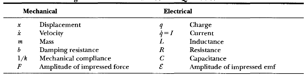Basically $x\to q$, and $m\to L$. The rest I know.
Fourier Series, any function can be represented as a series of sin and cos	$F(t)=a_0 + \sum_{n=1}^\infty a_n \cos(n\omega t) + \sum_{n=1}^\infty b_n \sin(n\omega t)$	Coefficients $a_n, b_n$ can be found using orthogonality
	$\mathcal{L}\left[ \sum \alpha_n x_n(t) \right]= \sum \alpha_n F_n(t)$	Then the above is useful because any driving force can be expressed as a Fourier series
		Proof: If $\mathcal{L}[x_n]=F_n(t)$, then use linearity

Special Note

When dealing with damping + driving force being discontinuous: $F_{drive}=H(0)$, then we can also analyze the question discontionusly:

• $t < 0$, $x=0$

• $t \ge 0$, we have EOM being:

  \[\ddot{x}+2\beta \dot{x}+\omega_0^2x=H(0)\]

  and solve normally

Then, an impulse $F_{drive}=I(0,1)=H(0)-H(1)$. Realize the EOM is then in the form of:

\[\mathcal{L}[x] = H(0)-H(1)\]

so it is a linear combination of solutions each for:

• $\mathcal{L}[x_1] = H(0)$
• $\mathcal{L}[x_2] = -H(1)$
• $x = x_1 + x_2$

Lastly, if we have a delta function as impulse:

\[\ddot{x}+2\beta \dot{x}+\omega_0^2x=\delta(t)\]

Consider again discontinuously, but now basically:

• $t<0$, $x=0$

• $t \ge 0$, we have one more constraint to satisfy as $\int_{\epsilon}^{\epsilon}\delta(t)=1$, integrating the EOM gives:

  \[\left. \frac{dx}{dt}\right|_{>0} - \left. \frac{dx}{dt}\right|_{<0}=1\]

Chapter 5

Condition	Equation	Comments
Conservative force	$\nabla \times F = 0$	Since $\oint F\cdot dr = \int \nabla \times F = 0$
Gravitational Potential	$-\nabla \Phi = \vec{g}$	$\Phi$ is the potential
	$U=m\Phi$
	$d\Phi = dW$	work done needed to bring unit mass in a field $g$ for a distance $d\vec{r}$
		proof by $dW=-\vec{g}\cdot d\vec{r}=\nabla \Phi \cdot d\vec{r}=d\Phi$
Computing gravitational Potential	$\phi = -G \int_V \frac{\rho(r’)}{r}dV’$	Basically comes from $\phi = -GM/r$
Poisson’s Equation	$\nabla^2\Phi = 4\pi G \rho$	True anywhere in space. Useful for computing gravitational force
	$\nabla \cdot g = -4\pi G\rho$	Same equation as above

Special Notes

A good way to compute/construct integrals for continuous body is to consider:

1. write out:

   \[d\Phi = -G\frac{dM}{r}\]

2. Figure out what is $dM$ in the geometry. For instance, if we have a circular disk

   

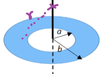
   Then

   \[\begin{align*} dM &=\rho dV\\ &=\rho r'\,dr'd\theta dz\\ &= \rho2\pi xdx \end{align*}\]

   where the last equality comes from integrating $d\theta$ and changing $r’=x$.

   • always remember you have two coordinates, $r’$ which is origin to the mass, and $r$ which is point of interest to the mass. Your goal is just two relate the two quantities in the integreal

3. Now the integral comes out easy, since $r^2 = x^2 + z^2$

   \[\begin{align*} \Phi &= \int -G\frac{dM}{r}\\ &= -G\int_a^b \frac{\rho (2\pi x)dx}{r}dx\\ &= -G\int_a^b \frac{\rho (2\pi x)dx}{\sqrt{x^2 + z^2}}dx \end{align*}\]

Another good way to solve for $\Phi$ is to use Poisson’s equation. Given some $\rho$, we know that:

1. By definition

   \[\nabla^2\Phi = 4\pi G \rho\]

2. If we have spherical symmetry, or whatever, write expand $\nabla^2 \Phi$

   \[\frac{1}{r^2}\frac{\partial }{\partial r}\left(r^2 \frac{\partial \Phi}{\partial r}\right) = 4\pi G \rho\]

   Note that now you are thinking from the origin towards outside, where $r$ is distance from origin.

   Then this is just an equation of $\Phi$. Solve for $\Phi$. e.g. For thin shell, area outside/outside the shell has $\rho = 0$, so we immediately have:

   \[\frac{\partial }{\partial r}\left(r^2 \frac{\partial \Phi}{\partial r}\right) = 0\]

   then inside the shell it should be $\frac{\partial \Phi}{\partial r} = 0$, and outside $\frac{\partial \Phi}{\partial r} = k/r^2$

   • the constant is found when solving for continuity at $r=r_0$ which at the shell

Chapter 6

Condition	Equation	Comments
Minimize $J=\int f(y_i, y_u’;x)\,dx$, such that $\frac{dJ}{d\alpha}=0$	$\frac{\partial f}{\partial y_i} - \frac{d}{dx}\frac{\partial f}{\partial y_i’}=0$
Minimize $J$, such that $\frac{dJ}{d\alpha}=0$, but also $\frac{df}{dx}=0$	\(\frac{d}{dx}(f - y'\frac{\partial f}{\partial y'})=0\)	Same as above, but can be easier to compute
Minimize $J$, such that $\frac{dJ}{d\alpha}=0$, but also with $j$ constraints $g_j(y_i;x)=0$	$\frac{\partial f}{\partial y_i} - \frac{d}{dx}\frac{\partial f}{\partial y_i’} + \sum_j \lambda_j(x)\frac{\partial g_j}{\partial y_i}=0$	Used when need constraint force, $\lambda_j(x)$ is some unknown
	$g_j(y_i;x)=0$	Useful since force of constraint is $Q_i = \sum_j \lambda_j(x)\frac{\partial g}{\partial y_i}$
Minimize $J$, such that $\frac{dJ}{d\alpha}=0$, but also with Integral $j$ constraints $\int_a^b g_j(y_i;x)=l$	$\frac{\partial f}{\partial y_i} - \frac{d}{dx}\frac{\partial f}{\partial y_i’} + \sum_j \lambda_j( \frac{\partial g}{\partial y}-\frac{d}{dx} \frac{\partial g}{\partial y’})=0$
	$\int_a^b g_j(y_i;x)=l$
Simple constraint optimization $J=J(y)$ is not an integral. Constraint is $g$	$\frac{\partial J}{\partial y_i} + \sum_j \lambda_j \frac{\partial g_j}{\partial y_i}=0$	Basically from that: $\nabla J = -\lambda \nabla g$

Special Notes

The equation to note here is the 3.1 one:

\[\frac{\partial f}{\partial y_i} - \frac{d}{dx}\frac{\partial f}{\partial y_i'} + \sum_j \lambda_j(x)\frac{\partial g_j}{\partial y_i}=0\]

notice that the sum is also over all the constraints.

Chapter 7

Condition	Equations	Comments
Hamiltonian’s minimizing least action $J=\int (T-U)dt$	$\frac{\partial L}{\partial q_i} - \frac{d}{dt}\frac{\partial L}{\partial q_i’}=0$	Basically $L=T-U\to f$, independent variable is often $t$ instead of $x$
		We are in generalized coordinate, where $q_1,…q_s$ represents the $s$ degrees of freedom of the system
Transformation between $q_i,…q_s$ to $x_1, …,x_n$ in cartesian	$x_i=x_i(q_1,…,q_s)$	e.g. $x=l\sin\theta$ for $\theta = q$ is the generalized coordinate
	\(x_i'=x_i'(q_1,...,q_s,q_i',...,q_s')\)
Legrangian with constraint $f(x_i;t)=0$	$\frac{\partial L}{\partial q_i} - \frac{d}{dt}\frac{\partial L}{\partial q_i’} + \sum_j \lambda_j(t)\frac{\partial f_j}{\partial q_i}=0$	Basically the analog
	$f_j(q_i;t)=0$
	$Q_i =\sum_j \lambda_j(t)\frac{\partial f_j}{\partial q_i}$	is the i-th force of constraint
Hamiltonian definition	$H \equiv \sum_j\dot{q}_j\frac{\partial L}{\partial \dot{q}_j} - L\equiv \sum_j\dot{q}_jp_j - L$	Derived from assuming a closed system, so that $\frac{\partial L}{\partial t} = 0$
1) if closed system, 2) If transformation equation is time independent, 3) and potential is only dependent on position	$E=H$	A faster way to write out $H$ if condition holds
Symmetry and In a closed system for Lagrangian	$\frac{\partial L}{\partial t}=0$, then $E$ is conserved	Time Homogenous
	$\frac{\partial L}{\partial x_i}=0$, $p_i$ momentum is conserved	Space Homogenous
	$\frac{\partial L}{\partial \theta}=0$, angular momentum is conserved	Space isotropic
Hamiltonian’s Equation	$p_j \equiv \frac{\partial L}{\partial \dot{q}_j}$	canonical momentum
	$H (q_i, p_i;t)\equiv \sum_j\dot{q}_jp_j - L$	Hamiltonian. Need to encode everything in the end to only include $H (q_i, p_i;t)$
	$\dot{q}_j = \frac{\partial H}{\partial p_j}$
	$\dot{p}_j = -\frac{\partial H}{\partial q_j}$	Equations of Motion because $p_j = \frac{\partial L}{\partial \dot{q}_j}$
Symmetry in Hamiltonian	$p_k$ is constant if $q_k \notin H$	Obviously comes from $\dot{p}_j = -\frac{\partial H}{\partial q_j}$
Viral Theorem, for averaging over (semi) periodic motion	$\lang T\rang =- \frac{1}{2}\lang \sum_i \vec{F}_i \cdot \vec{r}_i \rang$	For central force $F=kr^n$, can show that $\lang T\rang = \frac{n+1}{2}\lang U \rang$

Special Notes

The key equation for Lagrangian is, for $L=L(q_i, q_i’;t)$ for any generalized coordinate $q_i, q_i’$ (representing the $s$ degrees of freedom of the system)

\[\frac{\partial L}{\partial q_i} - \frac{d}{dt}\frac{\partial L}{\partial q_i'}=0,\quad i \in [0,s]\]

---

Hamiltonian comes from assuming a closed system, so $\frac{\partial L}{\partial t} = 0$, then using the fact that:

\[\frac{d}{dt}L = \sum_i \frac{\partial L}{\partial q_j}\dot{q}_j + \sum_j\frac{\partial L}{\partial \dot{q}_j}\ddot{q}_j + \frac{\partial L}{\partial t}\]

And using the Lagrangian

\[\frac{\partial L}{\partial q_i} - \frac{d}{dt}\frac{\partial L}{\partial \dot{q}_i}=0\]

Then you basically get:

\[\frac{d}{dt}\left(L- \sum_j \dot{q}_j \frac{\partial L}{\partial \dot{q}_j}\right)=0\]

Chapter 8

Conditions	Equations	Comments
Two body with central force $F=F(r)$, in the center of mass frame	$L=\frac{1}{2}\mu \vert \dot{\vec{r}}\vert ^2 - U(r)$	reduced mass $\mu-\frac{m_1m_2}{m_1+m_2}$
	$L=\frac{1}{2}\mu(\dot{r}^2+r^2\dot{\theta}^2)-U(r)$	The next step is to treat this as a one body with $m=\mu$
	Hence $p_\theta=0$, angular momentum conserved. $l=\mu r^2\dot{\theta}$	since it is cyclic in $\theta$
Kepler’s second law	$\frac{dA}{dt}=\frac{l}{2\mu}=\text{constant}$, areal velocity is constant	Only needs $F=F(r)$ to be true
		Derived from $dA=\frac{1}{2}r^2d\theta$
Equation of motion. Only requires a closed system and $F=F(r)$	$\dot{r}=\pm \sqrt{\frac{2}{\mu}(E-U)-\frac{l^2}{\mu^2r^2}}$	$\dot{r}=\dot{r}(r)$!
		Derived from conservation of energy
	$\theta(r)=\int \frac{\pm (\frac{l}{\mu r^2})}{\sqrt{2\mu (E-U-\frac{l^2}{2\mu r^2})}} dr$	$\theta=\theta(r)$!
	$\dot{\theta}=l/(\mu r^2)$	$\dot{\theta}=\dot{\theta}(r)$!, shown from conservation of angular momentum
Geometry of orbit $r$ from only $F(r)$	$\frac{d^2}{d\theta^2}\frac{1}{r} + \frac{1}{r} = -\frac{\mu r^2}{l^2}F(r)$
$r_{\min}, r_{\max}$ of orbit, so $r_{\min}\le r\le r_{\max}$	solve $E-U-\frac{l^2}{2\mu r^2}=0$	from putting $\dot{r}=0$, obtain two solutions
		for circular orbit, will find $r_{\min}, =r_{\max}$
Closed orbit if $\Delta \theta = \frac{b}{a}2\pi$, so it repeats itself	\(\Delta\theta(r)=2\int_{r_\min}^{r_\max} \frac{l/r^2}{\sqrt{2\mu (E-U-\frac{l^2}{2\mu r^2})}} dr\)	Can be used to show that if $U=r^{n+1}$, then closed iff $n=-2,+1$.
Effective Potential	$V(r)=U(r)-\frac{l^2}{2\mu r^2}$	Used so that $E-V$ gives you $\frac{1}{2}\mu\dot{r}^2$, which is kinetic energy in radial direction
From Now ON, we START to assume $F\propto r^{-2}$		All the previous results are true for any $F=F(r)$
Kepler’s First law	$\frac{\alpha}{r}=1+\epsilon\cos(\theta)$	relates $r,\theta$, and $l,E$!
	$\epsilon = \sqrt{1+\frac{2El^2}{\mu k^2}}$	$\epsilon = \epsilon(E)$! A constant!
	$\alpha = l^2 / (\mu k)$	$\alpha = \alpha(l)$! Also a constant
		Derived from performing the integral of $\theta = \theta (r)$
Geometry of Orbit if given $E$ or $\epsilon$	$\epsilon > 1, E > 0$	Hyperbola. Escapes!
	\(\epsilon =1, E = 0\)	Parabola, Just escapes!
	$0<\epsilon <1, V_{\min}<E<0$	Ellipse. Bounded orbit
	$\epsilon =0, V_{\min}=E$	Circular. Bounded.
For planetary elliptical motion	$a = \frac{\alpha}{1-\epsilon^2} = \frac{k}{2\vert E\vert }$	$a$ is half of the major axis. Determined once $E$ is known!
	$b = \frac{\alpha}{\sqrt{1-\epsilon^2}} = \frac{l}{\sqrt{2\mu \vert E\vert }}$	$b$ is half of the minor axis. Determined once $E$ is known!
	$r_\min = a(1-\epsilon)=\frac{\alpha}{1+\epsilon}$	Pedigree. Determined once $E$ or $\epsilon$ is known!
	$r_\max = a(1+\epsilon)=\frac{\alpha}{1-\epsilon}$	Apogee. Determined once $E$ or $\epsilon$ is known!
Total Energy of an orbit	$E= - k /(2a)$	Obvious if we use the equation above about $a$.
	$T=-\frac{1}{2}U$	From $E=T+U$ or from Viral theorem since we have a periodic orbit
Kepler’s Third Law	$\tau^2 = \frac{4 \pi^2 \mu}{k}a^3$	Period is completely determined by knowing one of the axis!
Stability of Circular Orbit, for $F=-k/r^n$	$(3-n)l^2/\mu > 0$, so $n < 3$	Basically, if you are stable at $r=r_0$, then $\frac{\partial V}{\partial r}\vert _{r_0}=0$ and $\frac{\partial^2 V}{\partial r^2}\vert _{r_0} < 0$, so that $\dot{r}$ is stable.
Stability of Circular Orbit at $r=\rho$, for $F=-\mu g(r)$	$\frac{F’(\rho)}{F(\rho)} + \frac{3}{\rho} > 0$	consistent with above
Precession due to force being $F=kr^{-2}+\rho(r)$	Precession angle is $\Delta = 2\pi \delta / \alpha$
	$\delta, \alpha$ comes from putting stuff into the equation $\frac{d^2}{d\theta^2}u + u = \frac{1}{\alpha}+u^2\delta$

Special Note

The following equations of motion is true for any $F=F(r)$:

\[\dot{r}=\pm \sqrt{\frac{2}{\mu}(E-U)-\frac{l^2}{\mu^2r^2}} = \dot{r}(r)\]

where $E, l$ are constants. Then, consider expressing $\frac{d\theta}{dr}=\dot{\theta}/\dot{r}$:

\[\theta(r)=\int \frac{\pm (l/r^2)}{\sqrt{2\mu (E-U-\frac{l^2}{2\mu r^2})}} dr\]

And this also holds in general:

\[\frac{d^2}{d\theta^2}\frac{1}{r} + \frac{1}{r} = -\frac{\mu r^2}{l^2}F(r)\]

(this can be shown by considering Lagrangian for $\dot{r}$ that $\frac{\partial L}{\partial r}-\frac{d}{dt}\frac{\partial L}{\partial \dot{r}}=0$, and use $u=\frac{1}{r}$ substitution). From there we also has the effective potential:

\[V(r)=U(r)-\frac{l^2}{2\mu r^2}\]

so that $E-V$ is the kinetic energy in radial direction, i.e. for $\frac{1}{2}\mu\dot{r}^2$.

---

Now, we start to assume that $F \propto r^{-2}$. Then we can say:

\[\frac{\alpha}{r}=1+\epsilon\cos(\theta)\]

derived from substituiung $U=-k/r$ and defined $u=1/r$ to compute:

\[\theta(r)=\int \frac{ l/r^2}{\sqrt{2\mu (E-U-\frac{l^2}{2\mu r^2})}} dr\]

Then, using areal velocity we can determine the period. Since we know:

\[\begin{cases} A=\pi a b\\ \frac{dA}{dt} = l/(2\mu)\\ \end{cases}\]

Then from using basically that $\tau = \int_0^\tau dt = \frac{2\mu}{l}\int_0^A dA$, we can show that:

\[\tau = \frac{2\mu}{l}\pi ab= \frac{2\mu \pi}{l}\sqrt{\alpha a} \to \tau^2 = \frac{4 \pi^2 \mu}{k}a^3\]

By basically substituting in the definition of $\alpha = l^2 / (\mu k)$.

---

Stability of Circular Orbit at $r=\rho$, for $F=-\mu g(r)$. The derivation essentially comes from reaching:

\[\ddot{r}-r\dot{\theta} = \ddot{r}-\frac{l^2}{\mu^2 r^3} = -g(r)\]

Then since it is a differential equation only of $r$, we consider apply some small perturbation away from equilibrium such that $r=\rho + x$, for small $x$. So that $\rho$ is equilibrium and we are interested in motion of displacement $x(t)$ from equilibrium.

Note

This technique is very general and useful for any given EoM: $\ddot{r}= f(r)$, as all you need to do is for $r=\rho + x$

• at equilibrium $0 = f(\rho)$
• compute $\ddot{x} = f(\rho + x)$, using (binomial) expansions for the RHS to get it to linear terms
• put into $\ddot{x}= - \omega^2 x$ form, and done.

Eventually you will reach something like:

\[\ddot{x}+\left[ \frac{3g(\rho)}{\rho} + g'(\rho) \right]x \approx 0\]

which is Oscillation equation with frequency

\[\omega^2_0 = \frac{3g(\rho)}{\rho} + g'(\rho)\]

which is only oscillatory if $\omega^2_0 > 0$.

---

Precession angle basically is solved by considering how many MORE angle do I need to get back from $r_\min$ to $r_\min$ of the next iteration. The book gives an example specifying the force, so check that. But the general idea is:

First since we have the force, we use:

\[\frac{d^2}{d\theta^2}u + u = \frac{1}{\alpha}+u^2\delta\]

then use successive approximation to solve $u$. This basically gives:

\[u = \frac{1}{\alpha}\left(1+ \epsilon \cos (\theta - \frac{\delta}{\alpha}\theta)\right)\]

Finally, to reach the same $r_\min$ means to reach the same $u$. So Basically it is just:

\[\theta - \frac{\delta}{\alpha}\theta = 2\pi \to \theta = 2\pi + \Delta\]

so the $\Delta$ is the precession angle.

Chapter 10

Conditions	Equations	Comments
Any quantity $\vec{Q}$ originates from inside the rotating frame	$\left(\frac{d\vec{Q}}{dt}\right){\text{fixed}}=\left(\frac{d\vec{Q}}{dt}\right){\text{rot}} + \vec{w}_{\text{sys}}\times \vec{Q}$	$\left(\frac{d\vec{Q}}{dt}\right)_{\text{rot}}$ is rate pf change of $\vec{Q}$ measured inside the rotating frame
		$\vec{w}_{sys}$ is the rotation of the rotating frame
$\vec{r}’$ be the inertial position vector and $\vec{r}$ is the rotating position vector	$\left(\frac{d\vec{r}’}{dt}\right){\text{fixed}}=\left(\frac{d\vec{R}}{dt}\right){\text{fixed}}+\left(\frac{d\vec{r}}{dt}\right)_{\text{fixed}}$
	$\vec{v}{\text{fixed}} = \vec{V} + \vec{v}{\text{rot}} + \vec{w} \times \vec{r}$	derived from above
		$\vec{w} \equiv \vec{w}{sys}$, and $\vec{V}=\left(\frac{d\vec{R}}{dt}\right){\text{fixed}}$
Experienced force $\vec{F}_{\text{eff}}$ in a rotating frame	$\vec{F}{\text{eff}}=m\vec{a}{rot}=\vec{F}-m\ddot{\vec{R}}f - m \dot{\vec{w}}\times \vec{r} - m\vec{w}\times (\vec{w} \times \vec{r})-2m\vec{w}\times\vec{v}{rot}$	$\vec{F}$ is the real force in inertial frame
	$\ddot{\vec{R}}_f = \vec{w}\times \dot{\vec{R}}_f = \vec{w}\times \vec{w}\times \vec{R}_f$	if $\vec{R}_f$ is from center of earth to its surface
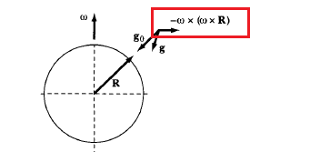
Simplified Experienced Force if on Earth	$\vec{F}{\text{eff}}=m\vec{a}{rot}=\vec{S}+m\vec{g} -2m\vec{w}\times\vec{v}_{rot}$	$\vec{S}$ real force other than gravity
	$\vec{g} \equiv \vec{g}_0 -\vec{w}\times [\vec{w} \times (\vec{R}+\vec{r})]$	for $\vec{r} « \vec{R}$ this value is a constant

Special Notes

The key derivation concept used throughout the chapter is to consider any quantity $\vec{Q}$ fixed w.r.t. the rotating frame:

\[\left(d\vec{Q}\right)_{\text{fixed}} = d\theta \times \vec{Q}\]

Hence, you get:

\[\left(\frac{d\vec{Q}}{dt}\right)_{\text{fixed}}= \vec{w}_{\text{sys}}\times \vec{Q}\]

Then if the quantity $\vec{Q}$ is measured to be moving within the rotating frame:

\[\left(\frac{d\vec{Q}}{dt}\right)_{\text{fixed}}=\left(\frac{d\vec{Q}}{dt}\right)_{\text{fixed}} + \vec{w}_{\text{sys}}\times \vec{Q}\]

---

In the equation:

\[\vec{F}_{\text{eff}}=m\vec{a}_{rot}=\vec{F}-m\ddot{\vec{R}}_f - m \dot{\vec{w}}\times \vec{r} - m\vec{w}\times (\vec{w} \times \vec{r})-2m\vec{w}\times\vec{v}_{rot}\]

the term:

• $-m\vec{w}\times (\vec{w} \times \vec{r})$ is basically a centrifugal force
• $-2m\vec{w}\times\vec{v}_{rot}$ is the Coriolis force that is perpendicular to $\vec{v}_{rot}$

All of those “forces” are fictitious force added such that the EoM would match our experimental observation in a rotating frame.

Centrifugal	Coriolis
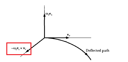Deflect gravity	Deflect velocity

---

Solving for two coupled equations (with opposite sign)

Consider equations like:

\[\begin{cases} \ddot{x} = 2 \omega_z \dot{y}\\ \ddot{y} = -2 \omega_z \dot{x} \end{cases}\]

If you consider $q = x+y$, then it doesn’t work as you will get:

\[\ddot{q} = \ddot{x} + \ddot{y} = -2\omega_z (\dot{x}-\dot{y})\]

But realize the trick that:

\[(i\dot{x} - \dot{y}) = i(\dot{x} + i\dot{y})\]

Therefore, if you consider $q = x + iy$, then it will magically work:

\[\ddot{q} = \ddot{x} + i\ddot{y} = -2 \omega_z i(\dot{x}+i\dot{y}) = -2\omega_z i\dot{q}\]

which you can solve.

Chapter 11

Conditions	Equations	Comments
(Recap) $\vec{L}$ in Lab/Fixed Frame $\vec{r}=\vec{r}f+\vec{r}{rot}$	$\vec{L} = \sum_i \vec{r}_i \times \vec{p}_i$	$\vec{r}_i$ is from origin of fixed frame to the body
	$\vec{L} = (\vec{r}{cm} \times \vec{p}{cm}) + I\vec{w}$	$I$ is inertia tensor will be defined then w.r.t to CoM frame
		Consistent with other derived parts
(Recap) $\vec{\tau}$ is Lab/Fixed Frame	$\vec{\tau}=(\vec{r}{cm}\times \vec{F}{total}) + (\sum_{i}\vec{r}_i’ \times \vec{F}_i)$	$\vec{r}_i’$ is the vector from CoM to the particle $i$ of the body
	$d\vec{L}/dt = \vec{\tau}$	Used for EoM
		Consistent with what we have
Kinetic Energy in Lab Frame, with Center of rotation at Frame $f$	$T = \frac{1}{2}\sum_{\alpha} m_{\alpha}V_f^2 + (\vec{V}f\cdot \vec{w})\times\sum\alpha m_{\alpha} \vec{r}{\alpha} + \frac{1}{2} \sum\alpha m_{\alpha}(\vec{w}\times \vec{r})^2$	$\vec{V}_f$ is the velocity of the moving frame itself
	$T = \frac{1}{2}MV_f^2 + \frac{1}{2} \sum_\alpha m_{\alpha}(\vec{w}\times \vec{r})^2 = T_{trans} + T_{rot}$	If moving frame is situated at Center of Mass, then $\sum_\alpha m_{\alpha} \vec{r}_{\alpha} =0$
Inertia Tensor	$T_{rot} = \frac{1}{2}\sum_{i,j}\omega_i\omega_j I_{ij} = \frac{1}{2}\vec{\omega}^TI\vec{\omega}$
	$I_{ij} =\sum_\alpha m_\alpha( \delta_{ij}\sum_{k} x_{\alpha, {k}{rot}}^2 -x{\alpha, {i}{rot}}x{\alpha, {j}_{rot}})$	example, $I_{11} = \sum_\alpha m_\alpha (x_{\alpha, 2}^2 + x_{\alpha, 3}^2)$
		replace the sum of $m_\alpha$ by integral $\rho dV$ for continues mass
		In the end, you will need to put $I$ and $\vec{\omega}$ into the same rotating axis-system (axis must be “not rotating” w.r.t $I$)
$\vec{L}$ w.r.t rotating axis fixed on the body without translation	$\vec{L}= \sum_{\alpha}\vec{r}{\alpha{rot}} \times \vec{p}{\alpha{real}} = I\vec{w}$	the body is only rotating
	$\vec{\tau} = \sum_{\alpha} \vec{r}{\alpha{rot}} \times \vec{F}{\alpha{real}}$	consistent with what we had before
		sometimes calculating $\sum_{\alpha}\vec{r}{\alpha{rot}} \times \vec{p}{\alpha{real}}$ could be easier
Kinetic Energy and Angular Momentum	$T_{rot} = \frac{1}{2}\vec{\omega}^TI\vec{\omega}= \frac{1}{2}\vec{\omega}\cdot \vec{L}$	Always remember that energies are useful for Lagrangian
Principle Moments of Inertia for some axis choice	$\mathbf{I}\vec{w}^* = I_\lambda \vec{\omega}^*$	if $\vec{\omega}$ happens to be along principle axis
	$\vec{\omega}^*$ along eigenvector	Basically principle axis direction = $\vec{w}$ along the eigenvector
Parallel Axis Theorem	$J_{ij} = I_{ij} + M[\vert \vec{a}\vert ^2 \delta_{ij} - a_ia_j]$	$\vec{a}$ is the vector from origin $Q$ to origin $O$ where $I_{ij}$ is defined
		example: $J_{11} = I_{11}+M[a_2^2 + a_3^2]$
Euler’s Angles	$\vec{x} = \mathbf{\lambda}\vec{x}’$, $\lambda$ is the rotational matrix	$\vec{x}$ is the rotational axis
	$\lambda = \lambda_\psi\lambda_\theta \lambda_\phi$	any $\vec{x}$ of the body rotating is the same as doing $\lambda\vec{x}’$ of the not-rotating body
		Any rotation $\vec{w}$ can be described by doing $\phi, \theta, \psi$ rotation
		Notice that $\phi, \theta, \psi$ points are not all in the direction of principle axis
	$\vec{w} = \begin{bmatrix} \dot{\phi}\sin\theta\sin\psi + \dot{\theta}\cos\psi\ \dot{\phi}\sin\theta\cos\psi - \dot{\theta}\sin\psi\ \dot{\phi}\cos\theta+\dot{\psi}\end{bmatrix}$, in body-fixed $\vec{x}$	Project $\vec{w}\phi = \dot{\phi}, \vec{w}\theta = \dot{\theta}, \vec{w}_\psi = \dot{\psi}$, into the principle/body frame $\vec{w}$
Euler’s equation for free body along principle axis	$(I_1 - I_2)\omega_1 \omega_2 - I_3 \dot{\omega}_3=0$	with no net force, only rotation
	$(I_2 - I_3)\omega_2 \omega_3 - I_1 \dot{\omega}_1=0$	since we are at principle axis, use the $\vec{w}$ found above
	$(I_3 - I_1)\omega_3 \omega_1 - I_2\dot{\omega}_2=0$
Euler’s equation for General body along principle axis	$(I_1 - I_2)\omega_1 \omega_2 - I_3 \dot{\omega}_3=\tau_1$	with net force causing a torque
	$(I_2 - I_3)\omega_2 \omega_3 - I_1 \dot{\omega}_1=\tau_2$	everything defined along principle axis
	$(I_3 - I_1)\omega_3 \omega_1 - I_2\dot{\omega}_2=\tau_3$
EoM of Force Free Motion of Symmetric Top $I_1=I_2$	$\dot\omega_1 = - \left( \frac{I_3-I_1}{I_1}\omega_3 \right)\omega_2$	Basically using force free Euler’s equatoin
	$\dot\omega_2 = \left( \frac{I_3-I_1}{I_1}\omega_3 \right)\omega_1$
	$\omega_3(t)=\text{const}$
Solution of Force Free Motion of Symmetric Top $I_1 = I_2$	$\omega_1(t) = A\cos (\Omega t)$	$\frac{I_3-I_1}{I_1}\omega_3 \equiv \Omega$
	$\omega_2(t) = A\sin (\Omega t)$	Precession as $\omega_1,\omega_2$ traces out a circle
	$\omega_3(t)=\text{const}$

Special Notes

To derive the total kinetic energy of a moving + rotating rigid body, start with considering expressing $\vec{v}_{\alpha}$ in the fixed/lab frame:

\[\vec{v}_{\alpha_{fixed}} = \vec{V}_f + \vec{v}_{rot} + \vec{\omega} \times \vec{r}_{rot}=\vec{V}_f + \vec{\omega} \times \vec{r}_{rot}\]

for the frame’s linear velocity being $\vec{V}f$ and $\vec{v}{rot}=\vec{0}$ since we are rotating with the frame itself.

Then, energy is simply:

\[\begin{align*} T &= \frac{1}{2}\sum_{\alpha} m_{\alpha}\vec{v}_{\alpha_{fixed}}^2\\ &= \frac{1}{2}\sum_{\alpha} m_{\alpha}V_f^2 + (\vec{V}_f\cdot \vec{w})\times\sum_\alpha m_{\alpha} \vec{r}_{\alpha} + \frac{1}{2} \sum_\alpha m_{\alpha}(\vec{w}\times \vec{r})^2\\ &= \frac{1}{2}MV_f^2 + (\vec{V}_f\cdot \vec{w})\times\sum_\alpha m_{\alpha} \vec{r}_{\alpha} + \frac{1}{2} \sum_\alpha m_{\alpha}(\vec{w}\times \vec{r})^2 \end{align*}\]

and often $\vec{V}f = \vec{V}{cm}$ if we choose the frame to be located at center of mass

---

When you have a purely rotating body without translation:

\[\vec{L} = \sum_{\alpha}\vec{r}_{\alpha_{rot}} \times \vec{p}_{\alpha_{real}}\]

for $\vec{r}\alpha$ is w.r.t the rotating axis and $\vec{p}\alpha$ is the real momentum in fixed frame.

Together with $\vec{\tau}$, we can write EoMs.

\[\vec{\tau} = \sum_{\alpha} \vec{r}_{\alpha_{rot}} \times \vec{F}_{\alpha_{real}}\]

---

Derivation of Parallel Axis Theorem

The idea is actually simple. Consider you have already $I$ with origin at $\mathcal{O}$. Then, you want to calculate at $\mathcal{Q}$:

\[\vec{r}_Q = \vec{a}+ \vec{r}_O \to X = \vec{a} + \vec{x} \quad \text{ for easier identification}\]

Then by definition:

\[\begin{align*} J_{ij} &=\sum_\alpha m_\alpha ( \delta_{ij}\sum_{k} X_{\alpha, {k}_{rot}}^2 -X_{\alpha, {i}_{rot}}X_{\alpha, {j}_{rot}})\\ &=\sum_\alpha m_\alpha \left[\delta_{ij}\sum_{k} (\vec{x}_{\alpha, {k}_{rot}}+\vec{a})^2 -(x_{\alpha, {i}_{rot}} + \vec{a})(x_{\alpha, {j}_{rot}} + \vec{a})\right] \end{align*}\]

Then extract out the term $I_{ij} =\sum_\alpha m_\alpha ( \delta_{ij}\sum_{k} x_{\alpha, {k}{rot}}^2 -x{\alpha, {i}{rot}}x{\alpha, {j}_{rot}})$ in the expression you will obtain that

\[J_{ij} = I_{ij} + M[|\vec{a}|^2 \delta_{ij} - a_ia_j]\]

---

Euler’s Angle and Rotation

Basically we can describe any rotation as $\phi, \theta, \psi$:

Then, if we project each $\vec{w}\phi = \dot{\phi}, \vec{w}\theta = \dot{\theta}, \vec{w}_\psi = \dot{\psi}$ back into body fixed frame:

\[\dot{\vec{\phi}} = \begin{bmatrix} \dot{\phi}\sin\theta\sin\psi \\ \dot{\phi}\sin\theta\cos\psi \\ \dot{\phi}\cos\theta\end{bmatrix}\] \[\dot{\vec{\theta}} = \begin{bmatrix} \dot{\theta}\cos\psi\\ - \dot{\theta}\sin\psi\\ 0\end{bmatrix}\] \[\dot{\vec{\psi}} = \begin{bmatrix} 0\\ 0\\ \psi\end{bmatrix}\]

which makes sense because graphically $\dot{\psi}$ is along the z’ axis (body fixed axis already). Then, adding all of them up, total rotation $\vec{w}$ is:

\[\vec{w} = \begin{bmatrix} \dot{\phi}\sin\theta\sin\psi + \dot{\theta}\cos\psi\\ \dot{\phi}\sin\theta\cos\psi - \dot{\theta}\sin\psi\\ \dot{\phi}\cos\theta+\dot{\psi}\end{bmatrix}\]

---

Euler’s equation for free body along principle axis

Using Lagrangian. Basically:

1. since there is no net force:

   \[\mathcal{L} = T - 0\]

2. Using principle axis

   \[T = \frac{1}{2} \vec{w}^TI\vec{w} = \frac{1}{2} \sum_i I_i \omega_i^2\]

   for now we are at $\vec{\omega}$ in principle axis

3. To express $\omega$ in that axis, we can employ easily:

   \[\vec{w} = \begin{bmatrix} \dot{\phi}\sin\theta\sin\psi + \dot{\theta}\cos\psi\\ \dot{\phi}\sin\theta\cos\psi - \dot{\theta}\sin\psi\\ \dot{\phi}\cos\theta+\dot{\psi}\end{bmatrix}\]

   which is already in that axis. So we have $\mathcal{L} = \mathcal{L}[\phi, \dot{\phi}, \theta, \dot{\theta}, \psi, \dot{\psi}]$

4. Use the Lagrangian EoM and obtain:

   \[\begin{align*} \frac{\partial T}{\partial \psi} - \frac{d}{dt}\frac{\partial T}{\partial \dot{\psi}} &= 0\\ \frac{\partial T}{\partial \vec{w}}\frac{\partial\vec{w}}{\partial\psi} - \frac{d}{dt}\frac{\partial T}{\partial \vec{\omega}}\frac{\partial\vec{w}}{\partial \dot{\psi}} &= 0\\ \sum_i\frac{\partial T}{\partial w_i}\frac{\partial w_i}{\partial\psi} - \frac{d}{dt}\sum_i\frac{\partial T}{\partial \omega_i}\frac{\partial \omega_i}{\partial \dot{\psi}} &= 0 \end{align*}\]

   and compute since we have $\omega, T$ as a function of the angles

5. Obtain:

   \[(I_1 - I_2)\omega_1 \omega_2 - I_3 \dot{\omega}_3=0\]

6. Permute it. (Do not try to compute the Lagrangian of $\theta, \phi$, which will be tough)

Chapter 12

Conditions	Equations	Comments
Coupled Oscillator of 2 Bodies (using algebra)	$\eta_1 = x_1 - x_2 \equiv C_1 e^{i\omega_1 t}+C_2 e^{-i\omega_1 t}$	Basically arrive at EoM and assume oscillatory solution
	$\eta_2 = x_1 + x_2 \equiv D_1 e^{i\omega_2 t}+D_2 e^{-i\omega_2 t}$
	$\omega_1 = \sqrt{(\kappa + 2 \kappa_{13} )/m}$	Solved from plugging in the solution back into EoM, obtaining the characteristic Equation
	\(\omega_2 = \sqrt{\kappa/m}\)
Coupled Oscillator of 2 Bodies (using linear algebra)	$\ddot{X} = MX$	EoM with Matrices
	$\ddot{X}=Q\Lambda Q^{-1}X\to Q^{-1}\ddot{X}=\Lambda Q^{-1}X$	where $Q^{-1}X$ is transforming into the eigenspace
		$Q^{-1}X$ is the space where motion are decoupled.
		Eigenvalue in $\Lambda$ is therefore the frequency of the normal modes
Splitting of energy	$\omega_0 = \sqrt{(\kappa + \kappa_{12})/M}$	frequency when one mass held fix
	$\omega_1 > \omega_0 > \omega_2$	splitting of frequency due to coupling
Weak Coupling, $\kappa_{12} « \kappa$	$\omega_1\approx \omega_0(1+\epsilon)$	Solved from $\omega_0 \approx (1+\epsilon)\cdot \sqrt{\kappa/m}$
	$\omega_2\approx \omega_0(1-\epsilon)$	$\epsilon = \kappa_{12}/(2\kappa)$
Coupled Oscillator of two body with weak coupling, with $x_1(0)=D,x_2(0)=0$	$x_1(t)=[D\cos(\epsilon \omega_0 t)]\cos(\omega_0 t)$	Solved from $(D/2)\cos (\omega_1 t) + (D/2)\sin (\omega_2 t)$ and matching initial conditions
	$x_2(t)=[D\sin(\epsilon \omega_0 t)]\sin(\omega_0 t)$
Loaded String	$m\ddot{z}j = - (T/d)(z{j-1}-2z_j + z_{j+1})$	$T/d \equiv \kappa$
	$\ddot{z} = c^2 \cdot {\partial^2 z}/{\partial x^2}$	Helmholtz equation from PDE
		$c^2 = \kappa d^2 / m$
	$z_n(x,t) = \sin(n\pi x/L)(A_n \cos (n\pi ct / L) + B_n \sin(n\pi ct/L))$	Fourier Series. Solve $A_n, B_n$ using orthogonality
		initial condition $z(0,t)=f(x),z_t(0,t)=g(x)$ needs to be specified
	$z_n(x,t) = D_n\sin(n\pi x/L)\sin(\omega_n t+ \theta_n)$	same solution using trig identity, $\omega_n = (n \pi c /L)$
	$z_n(x,t) = (D_n/2) \cdot [ \cos (n\pi (x-ct)/L) + \sin(n\pi (x-ct)/L)]$	compound angle from above

Special Notes

Weak Coupling:

Using Binomial expansion of $\sqrt{1+ 2\epsilon}$ you get:

\[\omega_0 =\sqrt{\frac{\kappa}{m}} (1+ \epsilon)\]

for $\epsilon = \kappa_{12}/(2\kappa)$. Then, express $\omega_1, \omega_2$ in terms of $\omega_0$ and we get what we want.

---

Loaded String

First we ignored gravity, then if we consider a string particle with mass $m$ at the $j$-th position

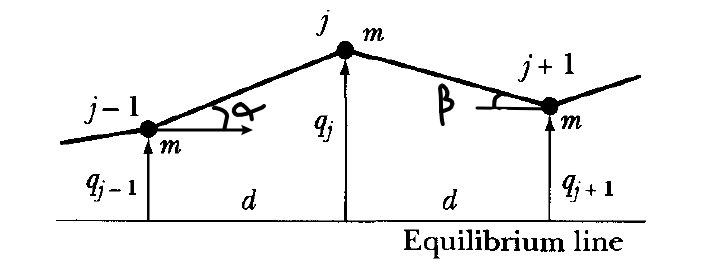
Then the vertical restoring force is given by, if the tension $T$ is the same:

\[\begin{align*} F_j &= -T \sin (\alpha) - T \sin (\beta)\\ &= -T \left( \frac{z_j - z_{j-1}}{d} \right)-T \left( \frac{z_{j+1} - z_{j}}{d} \right)\\ &= \frac{T}{d}(z_{j-1}-2z_j + z_{j+1} )\\ &= m \frac{d^2z}{dt^2} \end{align*}\]

But then, if we consider $z(x,t)$, we notice that the second derivative:

\[\begin{align*} \frac{\partial^2 z}{\partial x^2} &= \frac{1}{d}(\text{changes of rate of chage of $z(x)$})\\ &= \frac{1}{d}\left( \frac{(z_{j+1}-z_j) - (z_j - z_{j-1})}{d} \right)\\ &= \frac{1}{d^2}\left(z_{j-1}- 2z_j + z_{j+1}\right) \end{align*}\]

Then we get, letting $\kappa = T/d$

\[\frac{\partial^2z}{\partial t^2} = \frac{\kappa d^2}{m}\frac{\partial^2 z}{\partial x^2}\]

which if we define $c^2 = \kappa d^2 /m$, we get the Helmholtz equation:

\[\frac{\partial^2z}{\partial t^2} = c^2\frac{\partial^2 z}{\partial x^2}\]

which basically is solved using the technique in PDE with assuming $z(x,t)=\psi(x)h(t)$ and solve separately.