Week 1 - Logistics and Intro

Course Website http://www.cs.columbia.edu/~biliris/4111/21s/index.html
Exams are open book

Introduction

Some terms to know:

Definitions:

Database

a very large, integrated (relational) collection of shared data

DBMS - database management system

software that can manage database systems, with the advantage of reducing application development time, concurrent accesses, recovery from crashes, etc.

Data Models

a collection of concepts/structure for describing the data

for example, is it a graph (social network data)? A tree? A table?

Schema

a description of a particular collection of data, using the data model

It defines how the data is organized and how the relations among them are associated. It formulates all the constraints that are to be applied on the data.

Relational Data Model

basically a set of inter-related tables containing your data

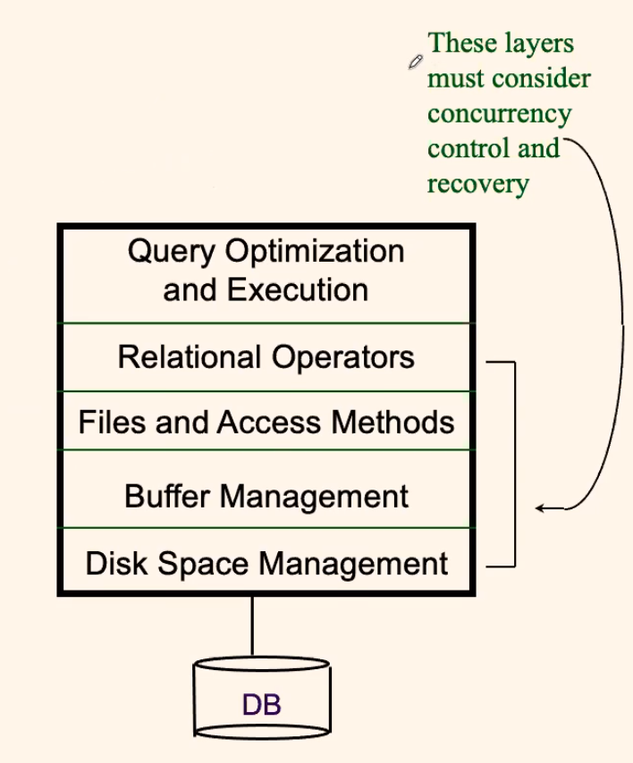
The levels of abstraction used in this course:

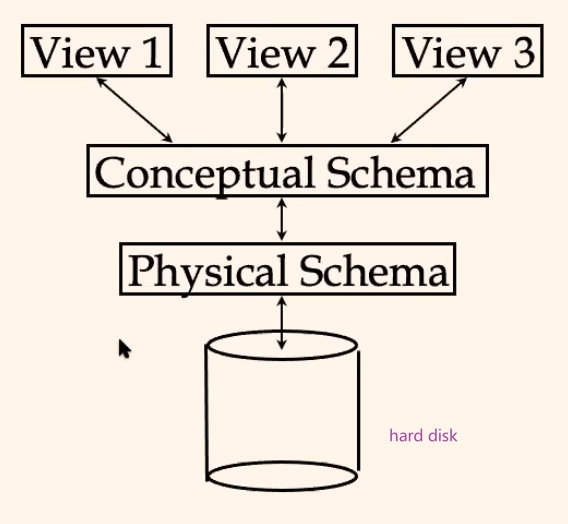
where:

Physical Database Schema − This schema pertains to the actual storage of data and its form of storage like files, indices, etc. It defines how the data will be stored in a secondary storage.
Conceptual/Logical Database Schema − This schema defines all the logical constraints that need to be applied on the data stored. It defines tables, views, and integrity constraints.

For example:

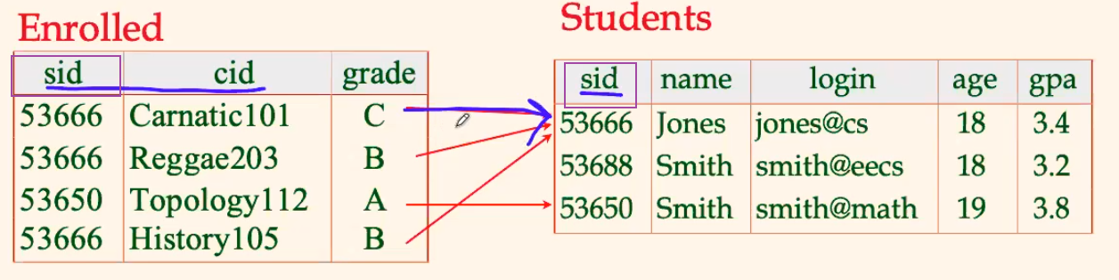
Consider a simple university database:

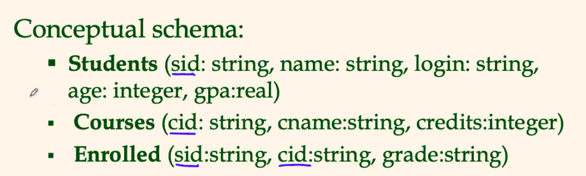
where:

the Enrolled table connects the Students and Courses table
so the conceptual schema tells you the organization of the table

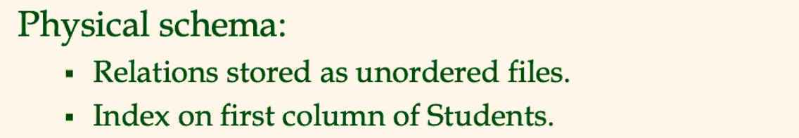
and:

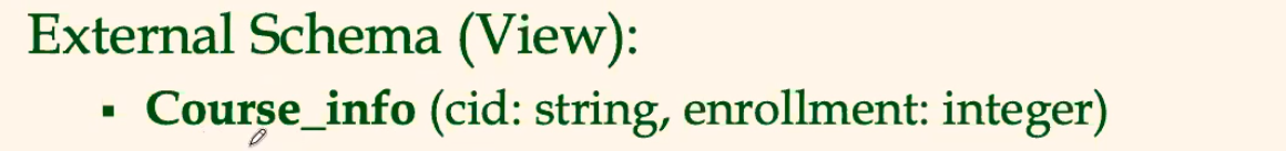
where:

this would be a computed table based on the actual tables we have (defined in the conceptual schema)

Definition: Data Independence

From the above, it can be implied that we need our application to be insulated from how the data is structured, so that the structure/organization should be intact

logical data independence - protection from changes in logical structure of data

physical data independence - protection from changes in physical structure of data

Definition: Transactions in Database

Transactions (a query/insert/… in database) is either committed or aborted (all-or-none)

This means it is important for having a concurrency control

Lock based protocol

Time-stamp protocol

Validation based protocol

This means that we will have the following structure for a DBMS:

Overview of Database Design

Conceptual Design (using ER Model)

What are the entities and relationships in the enterprise?
What are the integrity constraints or business rules that hold?
Can map an ER diagram into a relational schema?

Physical Database Design and Tuning

Considering typical workloads and further refine the database design

ER Diagram Basics

What is an ER Model? Why do we need it?

in short, it provides an abstract way of understanding the model without touching the data

Definition

Entity

real-world object, described using a set of attributes

Entity Set

a collection of entities that have the same attribute fields

each entity set has a key (could be a composite key as well)

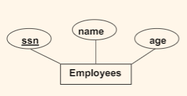
For example:

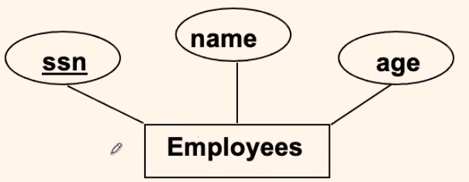
where:

employee would be an entity
employees would be a table containing the entity employee
the primary key would be the ssn

Definition

Relationship

Association among two or more entities.

Relationship Set

A collection of similar relationships

For example:

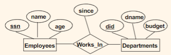
where:

Entity would be in square
Relationship would be in a diamond
Attributes would be in circle

Key and Participation Constraints

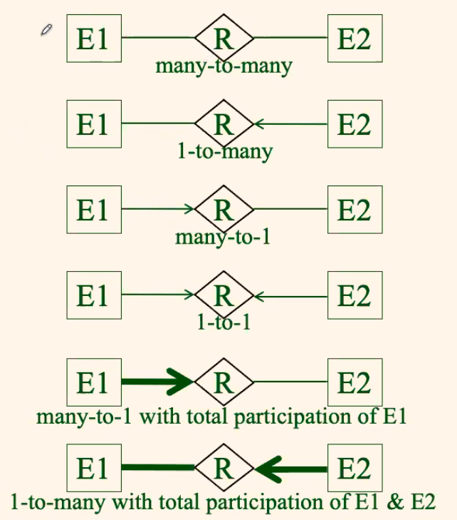
Before going to the details, first we talk about some notations:

The following relations are possible between one entity E another entity E’:

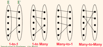
and in a more abstracted way:

where:

an arrow with head means upper-bounded with the 1-1 relationship
a bold line means a strong requirement that each entity must have a relation

For Example:

Now, we can go to key and participation constraints:

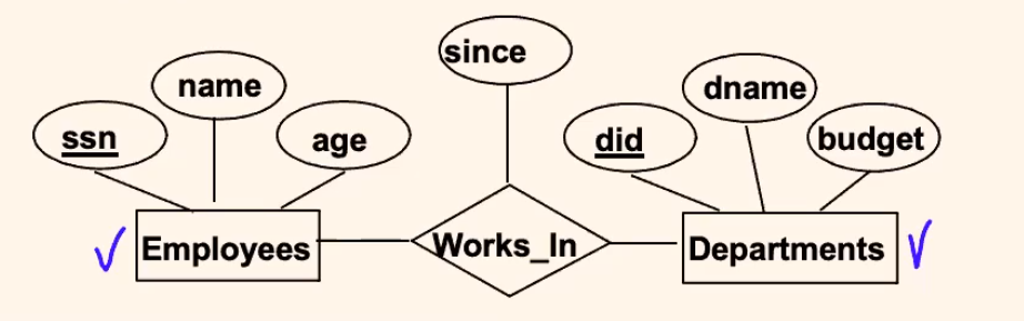
Key Constraint

the above diagram actually is a key constraint:

where:

since each department can participate at most one time in the relationship, each department has most one manager (or zero manager) = key constraint

each employee can manage zero or more departments

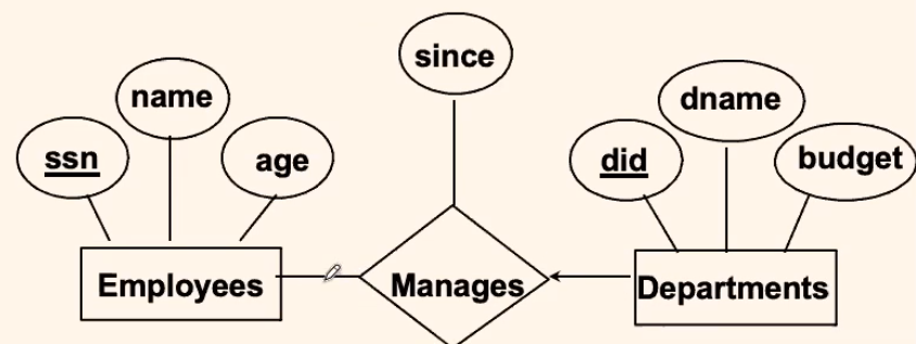
Participation Constraint:

where we see it means:

Each department must have a manager, because it participates exactly one = participation constraint

The participation constraint of Departments in Manages is said to be total (vs. partial).

For example:

Consider a more complicated case:

where, for the works_in relationship:

each Department participates at least once, meaning each department has at least one employee
each Employee works in at least one Department

Some summaries:

Weak Entities

Definition

A weak entity can be identified uniquely only by considering the primary key of another (owner) entity.

so that the weak entity does not “exist” automatically if the owner is deleted

Owner entity set and weak entity set must participate in a one-to-one or one-to–many relationship set (one owner, one or many weak entities; each weak entity has a single owner).

Weak entity set must have total participation in this identifying relationship set.

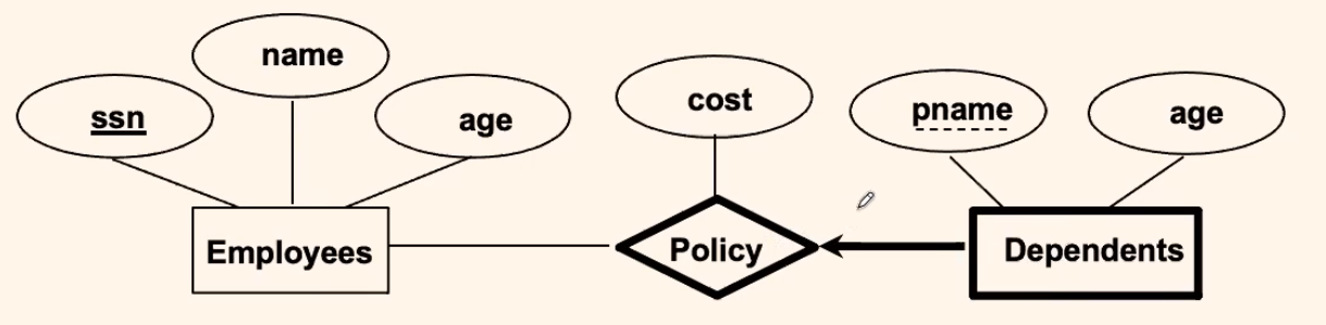
For example:

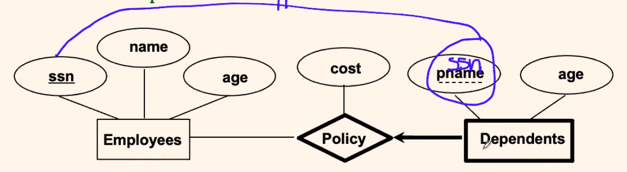
where:

the entity Dependent (weak entity) depends completely on the existence of an Employee
once a Policy/Employee is deleted, the Dependents of that policy/employee will automatically be disregarded

“Is A” Hierarchy

This is basically the same concept in OOP programming, in the context that:

children inherits the attributes of the parent

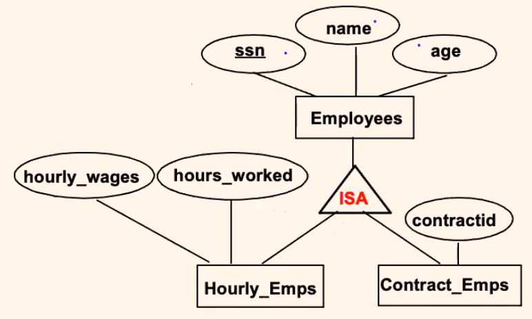
However, if using this design, you need to consider the following:

Overlap constraints:

Can Joe be an Hourly_Emps as well as a Contract_Emps entity? (Allowed/disallowed)

Covering constraints:

Does every Employees entity also have to be an Hourly_Emps or a Contract_Emps entity?(Yes/no)

Reasons for using ISA:

To add descriptive attributes specific to a subclass easily.
- e.g. easily look up an Hourly_Emp information (name) in the Employee table
To identify entities that participate in a relationship.

Week 2

ER Diagram Continued

Aggregation

General Constraint:

Usually, you should not relate relationships, you should only relate entities.

But what if you kind of need to?

For Example:

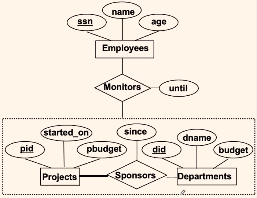
where:

we want the Employee to monitor not only the project, but also how the budget flow in this sponsorship. This means the Employee monitors pbudget+since+budget
- Practically, you could just have an aggregate entity consists of pid, did, since
so what we do is to view/aggregate the entire Project+Sponsors+Department as one entity

Definition: Aggregation

Allows us to treat a relationship set as an entity set for purposes of participation in (other) relationships.

Conceptual Design Using ER Model

Design choices:

Should a concept be modeled as an entity or an attribute or a relationship?
Identifying relationships: Binary or ternary? Aggregation?

Constraints in the ER Model:

A lot of data semantics can (and should) be captured.
- But some constraints cannot be captured in ER diagrams.

Entity vs. Attribute

For Example: Design Choice

Should address be an attribute of Employees or an entity (connected to Employees by a relationship)?

Ans: depends upon the use we want to make of address information, and the semantics of the data:

If we have several addresses per employee, address must be an entity
If the structure/components of it (city, street, etc.) is important, e.g., we want to retrieve employees in a given city, address must be modeled as an entity (since attribute values are atomic).
If all you need it to lookup/retrieve its entirety, then an attribute would suffice

Entity vs. Relationship

For Example

Consider the case: A manager gets a separate discretionary budget for each dept

First ER Diagram
- works

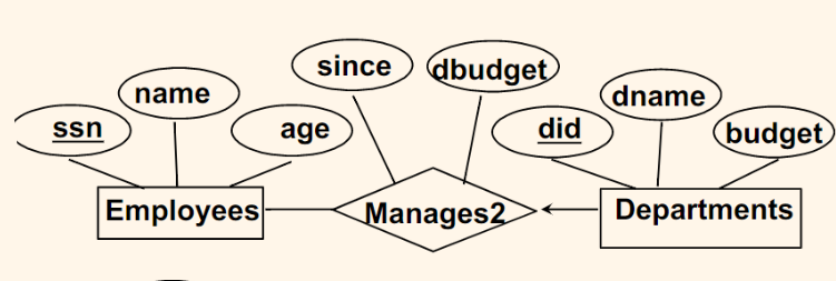
Note

the relational attribute dbudget (discretionary budget) depends on both the Employee and the Department. Hence, it is not an attribute of Department (e.g. a department might not have a manager, then there will be no budget)

Consider the case: A manager gets a discretionary budget that covers all his/her managed depts

then, the above diagram is bad, because:
- Redundancy: dbudget stored for each dept managed by manager.
- Misleading: Suggests dbudget associated with department-mgr combination.
In short, the dbuget depends on only the Employee who manages at least one departments

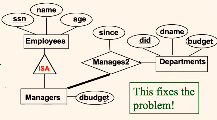
where:

the constraint above is: each Manager manages at least one Department. Hence, we have a thick line.

Binary vs. Ternary Relationship

In most of the time

A relationship would be no more than ternary, unless it IS EXTREMELY complicated

For Example: Binary Relationship

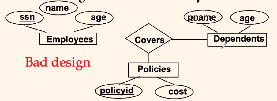
Consider: If each policy is owned by just 1 employee, and each dependent is tied to the covering policy

This diagram would be inaccurate
- we cannot constraint both: policy can only be owned by one employee and policy can have multiple dependents, i.e. the constraint is different for the relationships

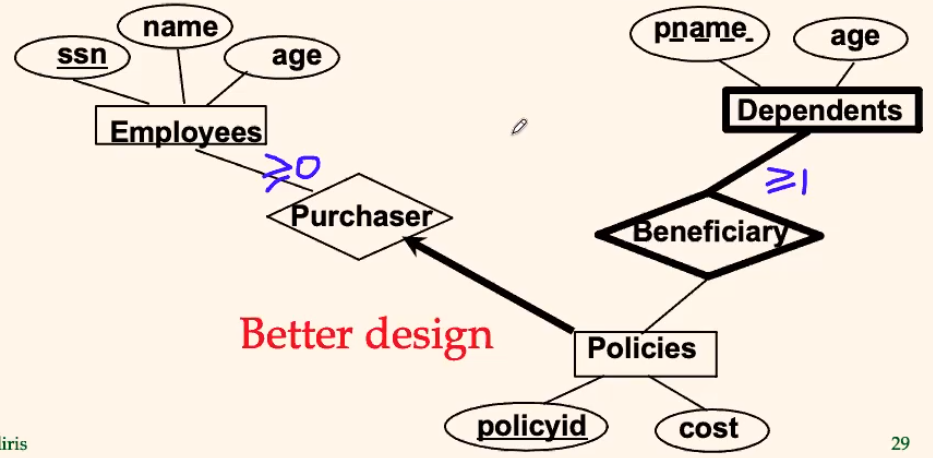
This diagram would work:
- now, since the constraint is different, we separated them into:
  - each policy is owned by one purchaser
  - policy can have multiple dependents

For Example: Ternary Relationship

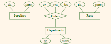
Consider: Orders relates entity sets Suppliers, Departments and Parts

An order <S,D,P> indicates: a supplier S supplies to a department D qtyof a part P at a certain cost on a certain date.
All of them have no constraints

Then this would work:

Summary:

When the relationships involved have the same constraint, then ternary relationship would work

Otherwise, you need to separate the relationships

For Example: Additional Constraints

Consider: Orders relates entity sets Suppliers, Departments and Parts, with these additional constraints

A department maintains a list of approved suppliers who are the only ones that can supply parts to the department
Each supplier maintains a list of parts that can supply

where:

again, since you should not relate relationships, you have the aggregates
however, a diagram cannot represent: the supplier of the department and the supplier of the parts is the same in one order. Therefore, for that you can only write a note in your diagram

Or alternatively:

where:

an INO would be useful for retrieving
each Invoice here can include more than one “orders”, so you can have multiple SD+SP associated with one invoice

Summaries on ER Model

Conceptual design follows requirements analysis
- Yields a high-level description of data to be stored
ER model popular for conceptual design
- Constructs are expressive, close to the way people think about their applications
Basic constructs: entities, relationships, and attributes (of entities and relationships).
Think about constraints
Some additional constructs: weak entities, ISA hierarchies, and aggregation.

Note:

There are many possible variations on ER model.

Relational Model and Database

By far, the relational model/database is the most widely used.

Major vendors:

Oracle, 44% market share (source: Gartner)
IBM (DB2 and Informix), 22%
Microsoft (SQL Server), 18%
SAP (bought Sybase in 2010), 4.1%
Teradata, 3.3%

A major strength of the relational model:

supports simple, powerful querying of data.
Queries can be written intuitively, and the DBMS is responsible for efficient evaluation

Definitions

Relational database:

a set of relations (tables)

A relation (table)

is a set of tuples (rows)

Schema: name of relation, name and type of each column, constraints.

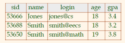
e.g. Students(sidstring, namestring, loginstring, ageinteger, gpareal).

#columns= degree / arity

Instance: the actual table (i.e., its rows) at a particular point in time.

All rows in a table are distinct.

columns could be the same

For Example

Basic SQL Query Language

For Example:

To find all 18 year old students, we write:

SELECT * FROM Students WHERE age=18

SELECT * FROM Students S WHERE S.age=18

S is used when you need to avoid ambiguities when querying multiple tables

CRUD Relations/Tables in SQL

To create a table:

CREATE TABLE Students(sid CHAR(20), name CHAR(20), login CHAR(10),age INTEGER,gpa REAL)  

To delete a table

DROP TABLE Students

To alter a table design:

ALTER TABLE Students ADD COLUMN firstYear: integer

Note

The schema of Students is altered if you change the structure

In the above, the structure is changed by adding a new field

every tuple in the current instance is extended with a null value in the new field.

To update data into a table:

INSERT INTO  Students (sid, name, login, age, gpa) VALUES (53688, ‘Smith’, ‘smith@ee’, 18, 3.2)

DELETE FROM Students S WHERE S.name = ‘Smith’

Integrity Constraints

You can specify constraints in your table, such that:

IC condition that must be true for any instance of the database
- ICs are specified when schema is defined
- ICs are checked when relations are modified
A legal instance of a relation is one that satisfies all specified ICs

Primary Key Constraint

Key

A set of fields is a key for a relation if:

No two distinct tuples can have same values in all key fields, and

This is any subset of the key becomes non-distinct, i.e. cannot be further decomposed

e.g. uni would be a key

Superkey

superkey is basically a union/superset of keys

e.g. uni+lastname would be a superkey

Candidate and Primary Key

Candidate key: any of the keys

there can be multiple candidate keys in a table

Primary key: one of the keys chosen DBA

there can only be one Primary key in a table

Primary/Unique/Not null

Syntaxes:

PRIMARY KEY (att1, att2, ...)

UNIQUE (att1, att2, ...)

att NOT NULL

For example: Primary Key

CREATE TABLE Enrolled (
    sid CHAR(20)
    cid  CHAR(20),
    grade CHAR(2), 
    PRIMARY KEY (sid,cid) 
)

means

For a given student and course, there is a single grade, or:
A student can only get one grade in an enrolled course

For example: Unique

CREATE TABLE Enrolled (
    sid CHAR(20),
    cid  CHAR(20),
    grade CHAR(2),
    PRIMARY KEY  (sid),
    UNIQUE(cid, grade) 
)

means

A student can only take one course, and
No two students can have the same grade in a course

For Example: Not Null

CREATE TABLE Students (
    age INTEGER NOT NULL
)  

Foreign Keys

Foreign keys keep referential integrity

Foreign Key

Fields in one tuple that is used to refer to another tuple’s PRIMARY KEY or UNIQUE.

Like a logical pointer, and it must exists. Otherwise, some optional actions will be taken (see below)

Referential integrity is achieved if all foreign key constraints are enforced, i.e., no dangling references.

For example

Consider the following referential integrity needed

CREATE TABLE Enrolled(
    sid CHAR(20),  
    cid CHAR(20),  
    grade CHAR(2),
    PRIMARY KEY  (sid,cid),
    FOREIGN KEY (sid) REFERENCES Students 
)

where:

the last line written in full is FOREIGN KEY (sid) REFERENCES Students (sid)

Now, to enforce referential integrity, consider:

What should be done if an Enrolled tuple with a non-existent student id is inserted?
What should be done if a Students tuple is deleted?

SQL/99 supports all 4 options on deletes and updates.

Default is NO ACTION (delete/update is rejected)
- e.g. you cannot delete 53666 of Enrolled or Student
CASCADE (also delete all tuples that refer to deleted tuple)
- e.g. deleting 53666 in Enrolled will also delete 53666 in Student
SET NULL /SET DEFAULT (sets foreign key value of referencing tuple)

CREATE TABLEEnrolled(
    sid CHAR(20),
    cid CHAR(20),
    grade CHAR(2),
    PRIMARY KEY  (sid,cid),
    FOREIGN KEY (sid)
    REFERENCES Students
    	ON DELETE CASCADE
    	ON UPDATE SET DEFAULT 
)

Views

View

A view is basically a ‘fictitious table’, such that

all of its data are computed at real time from another table at the time it is accessed

hence, it only stores definitions

Syntaxes

Creating a view

CREATE  VIEW  YoungGoodStudents (sid, name, gpa) AS(
    SELECT S.sid, S.name, S.gpa
    FROM  Students S
    WHERE  S.age < 20 and S.gpa >= 3.0
)

Deleting a view

DROP VIEW YoungGoodStudents

Since view dependent on actual tables:

How to handle DROP TABLE if there’s a view on the table?
- DROP TABLE command has options to let the user specify this.

Week 3

ER to Relational Database

How to we map what we have done in ER Diagram into Database?

Entity Sets to Tables

with:

CREATE TABLE Employees (
    ssn	CHAR(11),
    name CHAR(20),
    age INTEGER,
    PRIMARY KEY (ssn)
)

Relationship Sets to Tables

Now, relationships are basically tables with mostly foreign keys.

but now, we need to think about how to map the 1-to-many/many-to-1.,,, relationship

Many-to-Many Relationship:

with:

CREATE TABLE Works_In(
    ssn	CHAR(11),
    did	INTEGER,
    since	DATE,
    PRIMARY KEY (ssn, did),
    FOREIGN KEY (ssn) REFERENCES Employees,
    FOREIGN KEY (did) REFERENCES Departments
)

where:

PRIMARY KEY (ssn, did) essentially implements the many-to-many constraint

Key Constraint/ At Most 1 Participation

So that Departments can participate at most once

with:

three-table solution

CREATE TABLE  Manages (
    did  INTEGER,
    ssn  CHAR(11) NOT NULL,    // ok if NULL? No. Then the Manages table does not make sense
    since  DATE,
    PRIMARY KEY  (did),
    FOREIGN KEY (ssn) REFERENCES Employees,
    FOREIGN KEY (did) REFERENCES Departments
)

so that if it appears on this table, there is one manager. If a department does not have a manager, it is not in this table (this is the sole purpose of a relationship table)

two-table solution

CREATE TABLE  Dept_Mngr(
    did  INTEGER,
    dnameCHAR(20),
    budget  REAL, 
    ssn CHAR(11), // ok if NULL. Represents a Dept without Manager
    since  DATE,
    PRIMARY KEY  (did),
    FOREIGN KEY (ssn) REFERENCES Employees
)

since each Dept has a unique manager, combine Manages and Depts into one table.

now, a Dept can at most have one manager since it is an attribute that is nullable

Total Participation Constraint (=1/One to One)

Now, using the Dept_Mngr table is simply:

CREATE TABLE  Dept_Mngr(
    did  INTEGER,
    dname CHAR(20),
    budget  REAL,
    ssn CHAR(11) NOT NULL,
    since  DATE,
    PRIMARY KEY  (did),
    FOREIGN KEY  (ssn) REFERENCES Employees,
    ON DELETE NO ACTION
)

now, we have ssn being NOT NULL, so that each department has exactly one manager

if it is one-to-one, then it is basically an attribute

This means a relationship table would not capture the constraint anymore:

CREATE TABLE  Manages (
    ssn CHAR(11) NOT NULL,
    did  INTEGER,
    since  DATE,
    PRIMARY KEY  (did),
    FOREIGN KEY (ssn) REFERENCES Employees,
    FOREIGN KEY (did) REFERENCES Departments
) // Does not work

there is no constraint that forces ALL entries of Dept to appear here

Total Participation Constraint ($\ge$1)

Without Check constraint, this is not possible.

Consider the following:

CREATE TABLE  Dept_Mngr(
    did  INTEGER,
    dname CHAR(20),
    budget  REAL,
    ssn CHAR(11), // ssn is a PK, so no need to NOT NULL
    since  DATE,
    PRIMARY KEY  (did, ssn),
    FOREIGN KEY  (ssn) REFERENCES Employees,
    ON DELETE NO ACTION
)

this would work physically, but there would be redundancy, which would be a source of error for CRUD

dname CHAR(20) and budget REAL would be repeated

Similarily:

//3 tables (Emp, Dept, Manages)
CREATE TABLE  Manages (
    ssn CHAR(11),
    did  INTEGER,
    since  DATE,
    PRIMARY KEY  (did, ssn),
    FOREIGN KEY (ssn) REFERENCES Employees,
    FOREIGN KEY (did) REFERENCES Departments
)

which would not work since a relationship table cannot force total participation

Weak Entity to Tables

Reminder

A weak entity should only make sense by considering the PK of the owner

depends entirely on the existence of an owner

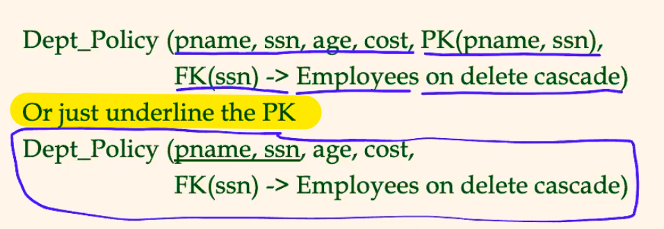
Consider:

with:

// Dependents and Policy are translated into ONE TABLE
CREATE TABLE  Dep_Policy (
    pname  CHAR(20),
    age  INTEGER,
    cost  REAL,
    ssn  CHAR(11),
    PRIMARY KEY  (pname, ssn),
    FOREIGN KEY  (ssn) REFERENCES Employees
    ON DELETE CASCADE
)

where:

Weak entity set and identifying relationship set are translated into a single table.
- so that entries in Dependents will also be deleted when the owner is gone
When the owner entity is deleted, all owned weak entities must also be deleted.

Alternatively:

if you want to keep the three table structure:

CREATE TABLE  Policies (
    policyid  INTEGER,
    cost  REAL,
    ssn  CHAR(11)  NOT NULL,
    PRIMARY KEY (policyid),
    FOREIGN KEY (ssn) REFERENCES Employees,
    ON DELETE CASCADE
)
CREATE TABLE Dependents(
    pname  CHAR(20),
    age  INTEGER,
    policyid  INTEGER,
    PRIMARY KEY (pname, policyid),
    FOREIGN KEY (policyid) REFERENCES Policies,
    ON DELETE CASCADE
)

so that:

When the owner entity is deleted, all owned weak entities together with policy are also be deleted.

Compact SQL Notation

This is only for writing to quickly clarify the design. This will not compile.

Examples include:

Note:

Never omit the always crucial PK, UNIQUE, NOT NULL and FK constraints

ISA Hierarchies

Reminder

This is basically the OOP concept of inheritance

Additionally, some constraints here include:

Overlap constraints: can an entry go into both children?

Covering constraints: does an entry in parent forces an entry in at least one of the children?

In general, this is not supported naturally by relational database, but there are some approaches:

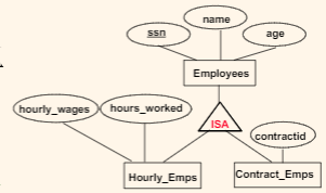
Emps(ssn, name, age, PK(ssn))

Hourly_Emps(h_wages, h_worked, ssn, PK(ssn), FK(ssn) -> Empson delete cascade)

Contract_Emps(c_id, ssn, PK(ssn), FK(ssn) -> Emps on delete cascade)

so that you basically manually creates the ISA relationship
Hourly_Emps(ssn, name, age, h_wages, h_worked)

Contract_Emps(ssn, name, age, c_id)

this makes queries easier, but there may be redundancy

However, the above design all depends on:

Overlap constraint: being both Hourly_Emps and Contract_Emps
- redundancy for the second design
- if not, no redundancy

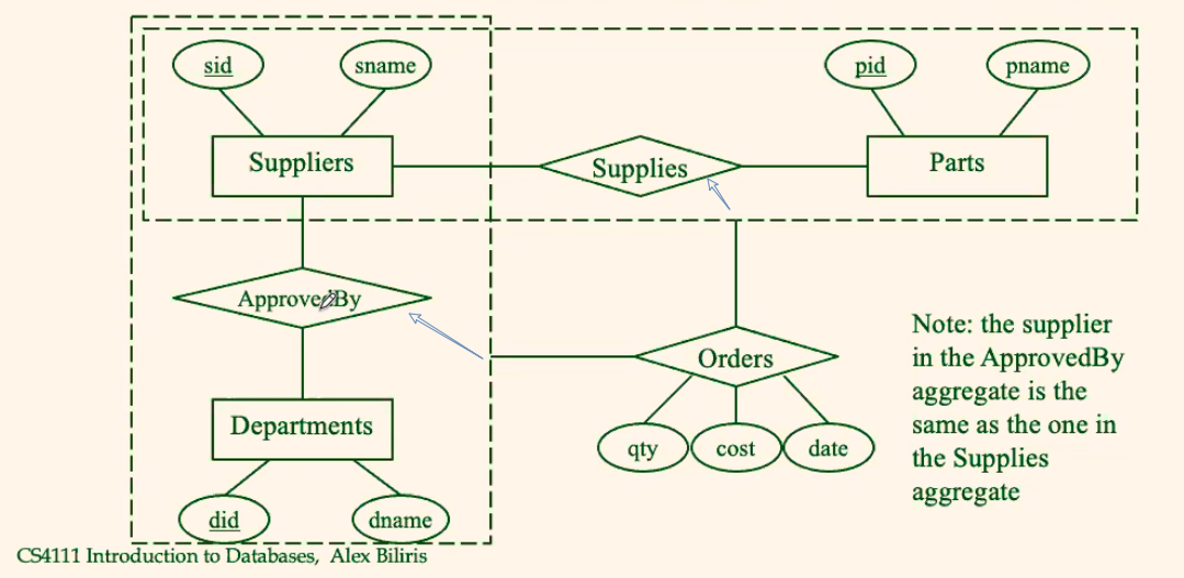
ER Design Examples

Orders example #1

Consider the following ER:

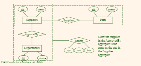
and we need that:

the supplier in the ApprovedBy aggregate is the same as the one in the Supplies aggregate

then the SQL tables would be:

Entities:

Suppliers (sid, sname)

Parts (pid, pname)

Departments (did, dname)
Relationships:

ApprovedBy(sid, did, FK(sid) -> Suppliers, FK(did) -> Departments)

Supplies (sid, pid, FK(sid) -> Suppliers, FK(pid) -> Parts)
Aggregate

``Orders (sid, did, pid, qty, cost, date,`

PK(sid, did, pid, qty, cost, date)

FK(sid, did) -> ApprovedBy,

FK(sid, pid) -> Supplies)

where:
- there is only one sid
- Orders relates to both ApprovedBy aggregate and Supplies aggregate by the two FK

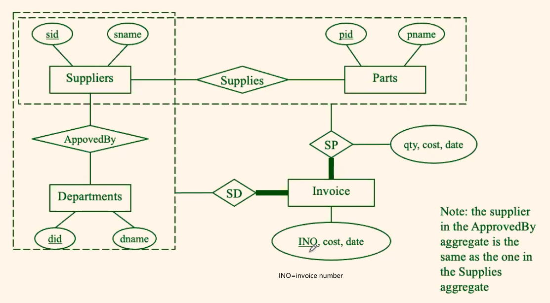
Orders example #2

Consider this example:

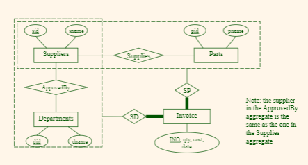
where:

Entities: same as above
Relationship: same as above
Aggregate:

Invoice(INO,

sid NOT NULL, did NOT NULL, pid NOT NULL, qty, cost, date,

PK(INO),

FK(sid, did) -> ApprovedBy,

FK(sid, pid) -> Supplies)

where:
- the idea is basically the same as before, the only advantage is that it only requires PK(INO) to get an entry, as compared to the previous PK(sid, did, pid, qty, cost, date)

Relational Query Languages

Query Languages

Query languages: Allow manipulation and retrieval of data from a database.

Query

Queries are applied to tables, and they output tables

i.e. the schema of the input and the output of a query is always the same, but the data inside might be different depending on data changes in the actual schema

Relational Algebra

In short, all tables are essentially sets, since each entry/row is unique.

Therefore, we have the following operations in SQL:

Basic operations:

Selection ($\sigma$): Selects a subset of rows from relation.
Projection ($\pi$): Deletes unwanted columns from relation.
Cross-product ($\times$): Allows us to combine two relations.
Set-difference ($\setminus$ or $-$): Tuples in reln. 1, but not in reln. 2.
Union ($\cup$): Tuples in reln. 1 and in reln. 2.

Additional operations:

Intersection $\cap$, join, division, renaming: Not essential, but (very!) useful.

Since each operation returns a relation, operations can be composed! (Algebra is “closed”.)

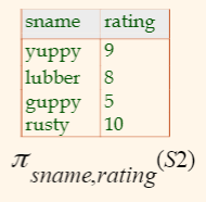
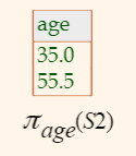
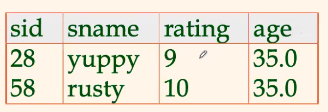
Operators Definitions

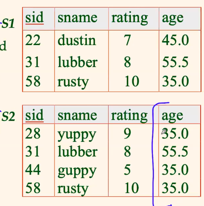
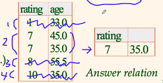
Projection

\[\pi_{sname, rating} (S2)\]
gives:
\[\pi_{age}(S2)\]
gives:

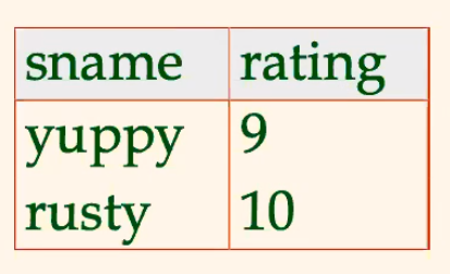
Selection

\[\sigma_{rating>8}(S2)\]
gives:
\[\pi_{sname, rating}(\sigma_{rating>8}(S2))\]
gives:

Set Operations are trivial

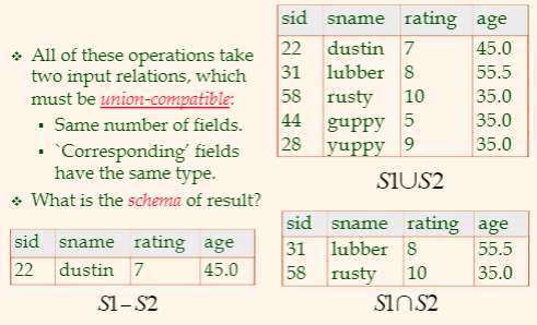
but note:

the only thing you need to make sure is that all entries are unique
tables need to be union-compatible
- contains the same number of attributes
- attributes are of the compatible type
- so that each row can be compared

Cartesian Product

Consider:

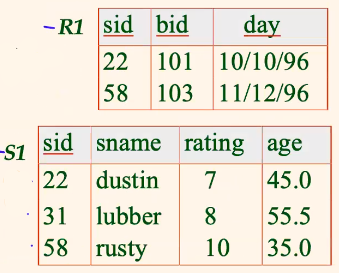
\[S1 \times R1\]
gives:

where:
- Conflict: Both S1 and R1 have a field called sid. (but the cartesian product does not care)
  - usually here you would rename: $$
    
    \rho(C(1\to sid1, 5\to sid2),S1\times R1)
    
    $$
- the cartesian product itself is usually useless. You will need to do some additionally operations.

Joins

Condition join is a combination of cartesian product and selection $$

\sigma_{condition}(R \times S) \equiv R \bowtie_{condition} S

$$
for example: $$

S1 \bowtie_{S1.sid < R1.sid}R1

$$ gives:

Note

This might be able to compute more efficiently

Equi-Join is a selection based on some equality
for example: $$

S1 \bowtie_{sid}R1

$$ gives:
Natural Join Equijoin on all common fields (fields with the same name and the same type)
for example: $$

S1 \bowtie R1

$$ gives the same:

since sid is the only common field for table S1 and table R1

Division

Let A have 2 fields, x and y; Bhave only field y: $$

A/B = { \lang x\rang\, \, \exist\lang x,y\rang \in A,\,\forall \lang y\rang \in B}

$$
i.e., A/B contains all x tuples (sailors) such that for every y tuple (boat) in B, there is an xy tuple in A.
i.e. returns x in A if and only if it has/tuples with all y in B
Not supported as a primitive operator. To express this as standard operation we had before:

Idea: For A/B, x value is disqualified if by attaching y value from B, we obtain an xy tuple that is not in A. $$

\pi_x(A) - \pi_x(\,(\pi_x(A)\times B)-A \,)

$$ where:
- $\pi_x(\,(\pi_x(A)\times B)-A \,)$ signifies the disqualified x values (xy tuple that is not in A.)
for example:

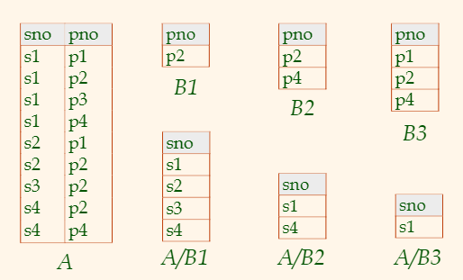
Example

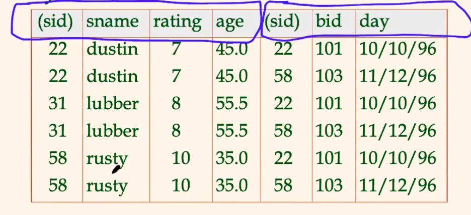
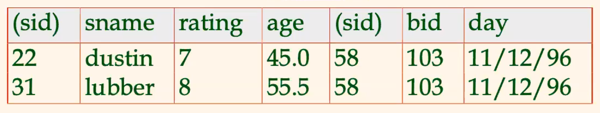
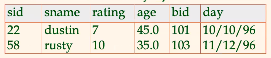
For Example: Find names of sailors who’ve reserved boat #103

so we have a Sailors and a Reserves table

Solution:

The straight-forward approach $$

\pi_{sname}((\sigma_{bid=103}Reserves)\bowtie Sailors)

$$
Splitting the above into individual steps: $$

\begin{align} &\rho(Temp1,\,\sigma_{bid=103}Reserves))
&\rho(Temp2,\,Temp1 \bowtie Sailors)
&\pi_{sname}(Temp2) \end{align}

$$
The “formula” approach (since many times, you simply joins first): $$

\pi_{sanme}(\sigma_{bid=103}(Reserves \bowtie Sailors))

$$

Choosing Which Query to Use

The expression itself must be correct

in the above case, all of them

The expression must be easy to read/understand for yourself

so that it there is an error, you can see it immediately

Do not care about performance yet

DBMS has internal query optimization made for you

For Example: Find names of sailors who’ve reserved a red boat.

So we have three tables, Sailors, Reserves, and Boat

Solution:

The straight-forward approach: $$

\pi_{sname}( (\sigma_{color=red}Boats)\bowtie Reserves \bowtie Sailors )

$$
The “formula” approach $$

\pi_{sname}(\sigma_{color=red}(Sailors \bowtie_{sid}Reserves \bowtie_{bid} Boats))

$$
etc.

For Example: Find names of sailors who’ve reserved a red or a green boat.

Solution:

The straight-forward approach: $$

\pi_{sname}( (\sigma_{color=red\,\lor\,color=green}Boats)\bowtie Reserves \bowtie Sailors )

$$
The “formula” approach $$

\pi_{sname}(\sigma_{color=red\,\lor\,color=green}(Sailors \bowtie_{sid}Reserves \bowtie_{bid} Boats))

$$
Computing the red and green boat separately, and then union the names

For Example: Find names of sailors who’ve reserved a red and a green boat.

Solution:

if this question is changed to and instead of or, then:
- changing $\lor$ to $\land$ for solution 1 and 2 would not work, because color is a singular value
changing the union to intersect would not work either, because:
- if there is sname=Mike, uid=1 who borrowed red boat, and a sname=Mike, uid=2 who borrowed green boat, then the intersection will also give Mike as the result, which is wrong
- therefore, you should use primary keys before the last step
\[\begin{align*} \pi_{sname}(\pi_{sname,sid} (\sigma_{red} (S \bowtie R \bowtie B)) \cap \pi_{sname,sid} (\sigma_{green} (S \bowtie R \bowtie B))) \end{align*}\]
where:
- $\pi_{sname,sid} (\sigma_{red} (S \bowtie R \bowtie B))$ selects correctly unique sailors who have reserved red boat
- $\pi_{sname,sid} (\sigma_{green} (S \bowtie R \bowtie B))$ selects correctly unique sailors who have reserved green boat

For Example: Find the names of sailors who’ve reserved all boats

Solution:

Using division: $$

\begin{align} &\rho(Tempsids, (\pi_{sid, bid} Reserves)/(\pi_{bid} Boats)) \end{align}
\[which gets all `sid` who has *reserved all boats*, since: - $(\pi_{sid, bid} Reserves)/(\pi_{bid} Boats)$ returns a tuple $\lang sid, bid\rang$ $\iff$ a $\lang sid \rang$ in $Reserves$ contains *columns* $\lang sid, bid\rang$ for all $\lang bid \rang$ in $Boats$ lastly, we do:\]
\pi_{sanme}(Tempsids \bowtie Sailors)

$$ to fetch the names.

SQL Queries

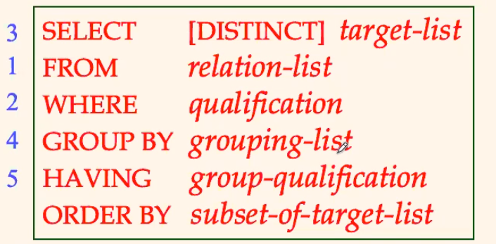
Basic SQL Structures

Basic Select Queries

It has the following structure

where:

by default, SQL will not remove duplicates from the query result. Therefore, sometimes you need to specify [DISTINCT] flag.

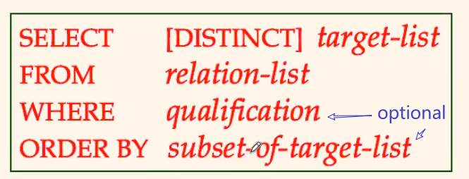
Basic Select Query Mechanism

From relation-list could be a list of relation/table names
- in that case, it computes the cartesian product of the given tables
WHERE qualification are comparisons using operators such as $>,<.=,etc$, connected with AND/OR/NOT
- in this case, it performs selection
SELECT target-list is a list of attributes of relations you wanted to have from the relation-list
- performs the projection
[DISTINCT] removes duplicate rows
ORDER BY just alters the sequence of the result presented

For Example:

Find the name of sailor who has rent the boat 103.

SELECT	S.sname 
FROM	Sailors S, Reserves R
WHERE	S.sid=R.sid AND R.bid=103

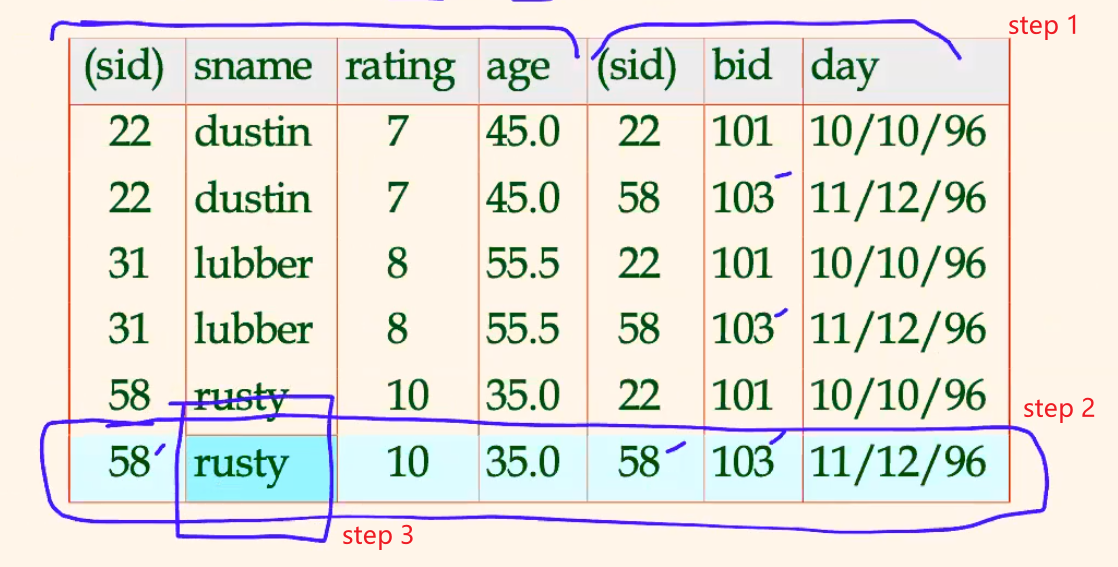
For Example:

Consider the following query:

SELECT	S.sid
FROM	Sailors S, Reserves R
WHERE	S.sid=R.sid

will the result contain duplicate sid?

Answer: yes, because a sailor could have reserved multiple boats, and by default SELECT statements do not remove duplicate results

Join Syntax

Inner Join

The below are all equivalent

SELECT	S.sname
FROM	Sailors S, Reserves R
WHERE	S.sid=R.sid AND R.bid=103

SELECT	S.sname
FROM    Sailors S JOIN Reserves R ON S.sid=R.sid
WHERE	R.bid=103

SELECT	S.sname
FROM    Sailors S INNER JOIN Reserves R ON S.sid=R.sid
WHERE	R.bid=103

Expression and Strings

For Example:

SELECT	age1=S.age-5, 
	2*S.age AS age2, 
	S.sid || ‘@columbia.edu’ AS email
FROM	Sailors S
WHERE	S.sname LIKE ‘B_%B’

where:

age1=S.age-5 computes S.age-5 and renames the column to age1
2*S.age AS age2 computes 2*S.age and renames the column to age2
S.sid||‘@columbia.edu’ AS email concatenates S.sid with @columbia.edu and renames the column to email
LIKE is used for string matching.
- _ stands for any one character and % stands for 0 or more arbitrary characters.
CAST is used for type casting
- CAST (S.rating as float)

Set Operations

Basic Syntax of Set Operations
query1 UNION [ALL] query2
query1 INTERSECT [ALL] query2
query1 EXCEPT [ALL] query2
where:

by default, duplicates are eliminated unless ALL is specified!

in this the only operation in SQL that automatically eliminates duplicates

of course, set operations work only when they are union compatible (same columns and types)

For Example

Find sids of sailors who’ve reserved a red or a green boat.

SELECT  R.sid
FROM  Boats B, Reserves R
WHERE  R.bid=B.bid AND B.color=‘red’
UNION
SELECT  R.sid
FROM  Boats B, Reserves R
WHERE  R.bid=B.bid AND B.color=‘green’

alternatively, only using WHERE:

SELECT	R.sid
FROM	Boats B, Reserves R
WHERE	R.bid=B.bid	AND	(B.color=‘red’ OR B.color=‘green’)

For Example

Find sids of sailors who’ve reserved a red boat but not a green boat.

SELECT  R.sid
FROM  Boats B, Reserves R
WHERE  R.bid=B.bid AND B.color=‘red’
EXCEPT
SELECT  R.sid
FROM  Boats B, Reserves R
WHERE  R.bid=B.bid AND B.color=‘green’

alternatively, only using WHERE

SELECT	R1.sid
FROM	Boats B1, Reserves R1,Boats B2, Reserves R2
WHERE	R1.sid=R2.sid AND R1.bid=B1.bid AND R2.bid=B2.bid 
	AND (B1.color=‘red’ AND NOT B2.color=‘green’)

note that we needed two pairs to tables, Boats B1, Reserves R1,Boats B2, Reserves R2, since for a table there is only one value for color

i.e. each record can only capture one color. Therefore, we need two tables and combine the result using sid and bid. (R1.sid=R2.sid AND R1.bid=B1.bid AND R2.bid=B2.bid )

Nested Queries

Nested Queries can happen in basically any where, including:

SELECT
FROM
WHERE
etc.

Note

In general, since we have a nested query, the scope of variables look like.

SOME QUERY with Var(S, T)

For example:

SELECT 	S.sname /* only S is visiable */
FROM 	Sailors S
WHERE 	S.sid IN (SELECT  R.sid /* S and R is visible */
                  FROM  Reserves R
                  WHERE  R.bid IN (SELECT B.bid /* S, R, B are all visible */
                                   FROM Boats B
                                   WHERE B.color=red)

where:

again, we are doing:
```
WHERE S.sid IN (SOME OTHER QUERY RESULT)
```
and that the return type of SOME OTHER QUERY RESULT has to match the type/format of S.sid

Nested Queries and IN

IN

essentially, xxx IN (some query) means only keeping values of xxx if it is the set of some query

and since this is basically a set operation, the types of xxx and some query has to be union compatible

the negation will be NOT IN

Consider the problem:

Find names of sailors who’ve reserved boat #103:

SELECT	S.sname
FROM	Sailors S
WHERE	S.sid IN (
    SELECT s.sid
    FROM Reserves R
    WHERE R.bid = 103
)

Rewriting INTERSECT with IN

Consider:

Find id/name of sailors who’ve reserved both a red and a green boat:

SELECT 	S.sid, S.sname
FROM	Sailors S
WHERE	S.sid IN (SELECT	R2.sid
                  FROM  Boats B2, Reserves R2
                  WHERE  R2.bid=B2.bid AND  B2.color=‘red’) 
                  AND
        S.sid IN (SELECT  R2.sid
                  FROM  Boats B2, Reserves R2
                  WHERE  R2.bid=B2.bid AND  B2.color=‘green’) 

where:

basically you are doing S.sid is in both the sets (results of the inner queries)
Similarly, EXCEPT/``MINUS queries re-written using NOT IN`.

Nested Queries and FROM

Consider the same problem

Find names of sailors who’ve reserved boat ``#103`:

SELECT	S.sname
FROM	Sailors S, (SELECT sid FROM Reserves WHERE bid=103) T
WHERE	S.sid=T.sid

notice that:

the line:

FROM	Sailors S, (SELECT sid FROM Reserves WHERE bid=103) T
WHERE	S.sid=T.sid

did a natural join on sid from the two tables S,T

Note
if and only if the inner query SELECT sid FROM Reserves WHERE bid=103 results in only one row/result, then it would be also correct to say:
SELECT	S.sname
FROM	Sailors S, (SELECT sid FROM Reserves WHERE bid=103) T
WHERE	S.sid=T

Multi-level Nested Queries

Consider:

SELECT 	S.sname
FROM 	Sailors S
WHERE 	S.sid IN (SELECT  R.sid
                  FROM  Reserves R
                  WHERE  R.bid IN (SELECT B.bid
                                   FROM Boats B
                                   WHERE B.color=red)

and it basically does “Find names of sailors who have reserved a red boat”.

Nested Queries with Correlation

Exists and Unique

EXISTS checks for empty set

returns true if table is not empty

UNIQUE checks for duplicate tuples

returns true if there are no duplicate tuples or the table is empty

Consider the problem

Find names of sailors who’ve reserved boat #103:

SELECT	S.sname
FROM	Sailors S
WHERE   EXISTS (SELECT	*
                FROM	Reserves R
                WHERE	R.bid=103 AND S.sid=R.sid)

where:

this is nested query with correlation, because the inner query WHERE R.bid=103 AND S.sid=R.sid correlates/uses S.sid which is of the outer query

therefore, since it used S.sid=R.sid, this is what happened:

SELECT	S.sname
FROM	Sailors S
WHERE   "If each S.sid EXISTS IN (SELECT	*
                		 	     FROM	Reserves R
               					 WHERE	R.bid=103 AND S.sid=R.sid)"

Similarly:

SELECT	S.sname
FROM	Sailors S
WHERE   UNIQUE (SELECT	R.bid
                FROM	Reserves R
                WHERE	R.bid=103 AND S.sid=R.sid)

Finds sailors with at most one reservation for boat ``#103. Since UNIQUE returns TRUE` if and only if the row is unique or empty.

and the correlation S.sid=R.sid can be translated to:

SELECT	S.sname
FROM	Sailors S
WHERE   "If each S.sid has UNIQUE data of (SELECT	R.bid
               							FROM	Reserves R
                						WHERE	R.bid=103 AND S.sid=R.sid)"

Nested Queries with Set Comparison

ANY, ALL Operations

<op> ANY returns true to the row if any of the comparison is true

<op> ALL returns true to the row if all of the comparison is true

For example:

Find sailors whose rating is greater than that of some sailor called “Mike”

SELECT	*
FROM	Sailors S
WHERE	S.rating > ANY (SELECT	S2.rating
                        FROM	Sailors S2
                        WHERE	S2.sname=‘Mike’)

where:

S.rating > ANY (SELECT S2.rating ...) returns true to a row of Sailors S if S.rating is larger than any S2.rating entry in the subquery’s table.

Division in SQL

In short, division is not supported naturally. Therefore, you need to do complicated queries.

For Example

Find sailors who’ve reserved all boats.

SELECT	S.sname
FROM	Sailors S
WHERE  	NOT EXISTS
		((SELECT	B.bid
          FROM  Boats B)
         EXCEPT
         (SELECT	R.bid
          FROM	Reserves R
          WHERE R.sid=S.sid))

which basically does:

SELECT	S.sname
FROM	Sailors S
WHERE  	NOT EXISTS
		( ALL_BOAT_IDs
         EXCEPT (Minus)
           ALL_BOAT_IDs_RESERVED_BY_A_SAILOR)

then NOT EXISTS does:

SELECT	S.sname
FROM	Sailors S
WHERE  	TRUE IF_BELOW_IS_EMPTY
		( ALL_BOAT_IDs
         EXCEPT (Minus)
           ALL_BOAT_IDs_RESERVED_BY_A_SAILOR)

Note

usually, when a query involves the ALL condition, the natural thinking shout be using DIVISION

However, since DIVISION is not supported naturally, when need to often compute the opposite, and minus it.

Aggregate Operators

Supported Aggregates

COUNT(*), COUNT( [DISTINCT] A)

counts the number of rows/distinct rows of a all columns/column A

SUM( [DISTINCT] A)

AVG( [DISTINCT] A)

MAX(A), MIN(A)

Reminder:

the SELECT part of a query is executed the last.

For Example

Number of sailors
```
SELECT  COUNT (*)
FROM  Sailors 
```

Average age of all sailors whose rating is 10:

SELECT	AVG (age)
FROM	Sailors
WHERE 	rating=10

Name of sailors with maximum/highest rating

SELECT 	S.sname
FROM 	Sailors S
WHERE	S.rating = (SELECT MAX(S2.rating) 
                    FROM  	Sailors S2)

Advanced SQL Constraints

Some basic SQL constraints have been covered in Integrity Constraints.

CHECK Constraints

Check Constraint

Attribute-based CHECK constraints involve a single attribute

it is basically a boolean expression, and it must evaluate to true for all rows of an attribute that has this constraint.

If the constraint does not mention any attribute, it applies to the entire table

e.g. if you use things like CHECK((SELECT COUNT(*) FROM Sailors) < 100)

If any table in the CHECK constraint is empty (i.e. just created with no data yet), then CHECK constraints automatically evaluate to true

e.g. CHECK((SELECT COUNT(*) FROM Sailors) > 100) is true for empty table

For Example

CREATE TABLE   Sailors (
    sid	INTEGER,
    rating	INTEGER,
    age REAL CHECK(age >= 17), /* all rows must have age >= 17 */
    PRIMARY KEY  (sid),
    CONSTRAINT	valid_ratings
    CHECK(rating >= 1 AND rating <= 10)
)   

where:

CHECK constraints can optionally be named. For example:

CONSTRAINT	valid_ratings
CHECK(rating >= 1 AND rating <= 10)

the position of CHECK constraints does not matter. It can be at the end as well.

For Example:

You can also check tuples:

CREATE TABLE   Sailors (
    sid	INTEGER,
    rating INTEGER CHECK (rating >= 1 AND rating <= 10),
    age REAL CHECK(age >= 17), /* all rows must have age >= 17 */
    PRIMARY KEY  (sid),
    CHECK( NOT (rating > 5 AND age < 20) ),
    CHECK( NOT (rating > 7 AND age < 25) )
)   

CHECK with SQL Queries

For Example

CREATE TABLE   Sailors (
    sid	INTEGER,
    rating INTEGER CHECK (rating >= 1 AND rating <= 10),
    age REAL CHECK(age >= 17), /* all rows must have age >= 17 */
    PRIMARY KEY  (sid),
    CHECK( NOT (rating > 5 AND age < 20) ),
    CHECK( NOT (rating > 7 AND age < 25) ),
    CHECK((SELECT COUNT(*) FROM Sailors) < 100)
)   

which constraints the number of sailors to 100.

Note:

By the definition of CHECK, the below will be true for empty table

CREATE TABLE   Sailors (
    sid	INTEGER,
    rating INTEGER CHECK (rating >= 1 AND rating <= 10),
    age REAL CHECK(age >= 17), /* all rows must have age >= 17 */
    PRIMARY KEY  (sid),
    CHECK( NOT (rating > 5 AND age < 20) ),
    CHECK( NOT (rating > 7 AND age < 25) ),
    CHECK((SELECT COUNT(*) FROM Sailors) > 100) /* true for empty table */
)   

For Example

CREATE TABLE  Reserves (
    sid	INTEGER,
    bid	INTEGER,
    day	DATE,
    PRIMARY KEY  (sid, bid,day),
    FOREIGN KEY (sid) REFERENCES Sailors,
    FOREIGN KEY (bid) REFERENCES Boats,
    CONSTRAINT noInterlakeRes /* this checks for each row of Reserves table */
    CHECK( 'Interlake' <> (SELECT  B.bnameFROM  Boats B WHERE  B.bid=bid) ) 
)

which basically means you cannot reserve the boat ‘Interlake’

note that (SELECT B.bnameFROM Boats B WHERE B.bid=bid) returns only a single row for each bid, so you can directly compare with a string ‘Interlake’.

CHECK with Assertion

In short, when you have a CHECK constraining multiple tables, the problem comes:

in which table should you put the constraint?
If any table in the CHECK constraint is empty, then CHECK constraints automatically evaluate to true. This will cause buggy behavior

Assertion

Often used for creating CHECK constraints for multiple tables

Does not automatically evaluate to true if any table is empty

hence fixes the bug

For Example: The Wrong Approach

I want to create a small club, which that number of sailors + boat $<$ 100

the Wrong Approach:

CREATE TABLE   Sailors (
    sid	INTEGER,
    rating  INTEGER,
    age  REAL,
    PRIMARY KEY (sid),
    CHECK ( (SELECT COUNT (*) FROM Sailors) + (SELECT COUNT (*) FROM Boats) < 100) )
)

which will be buggy if one of the table Sailors/Boats is empty, this will be always true

the Correct Approach:

CREATE ASSERTION  smallClub CHECK  (
    (SELECT COUNT (*) FROM Sailors) + (SELECT COUNT (*) FROM Boats) < 100 
)

Using Assertion for Total Participation

For Example

where we need:

each sailor reserves at least one boat (total participation)

CREATE ASSERTION  BusySailors (
	CHECK (
        NOT EXISTS (SELECT sid
                    FROM Sailors
                    WHERE sid NOT IN (SELECT sid
                                      FROM Reserves ))
    )
)

which basically means:

CREATE ASSERTION  BusySailors (
	CHECK (
        NOT EXISTS (SAILOR_SID_WHO_HAS_NOT_NOT_RESERVED_A_BOAT)
    )
)

then the NOT EXISTS means:

CREATE ASSERTION  BusySailors (
	CHECK (
        IS_EMPTY (SAILOR_SID_WHO_HAS_NOT_NOT_RESERVED_A_BOAT)
    )
)

Advanced SQL Queries

Group By

So far, we’ve applied aggregate operators to all (qualifying) tuples. Sometimes, we want to apply the aggregate operators to each of several groups of tuples.

e.g. AVERAGE GPA for students based on different ages (group)

For Example

Task: Find the age of the youngest sailor for each rating level.

You would like to do this (but you cannot):

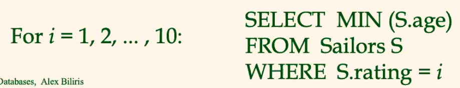
where:

it does not work for all times because:
1. often, we do not know what range of $i$ would this take
2. often, the values of $i$ might not be integers/equally spaced

Therefore, we need to solve it by using GROUP BY

Queries with Group By

Now, it looks like this:

and it evaluates from:

FROM (trivial)

WHERE (trivial)

SELECT, basically a projection, but it must make sense for groups. Target-list/Result list here must contains/returns either:

attribute names mentioned in grouping-list, or

terms with aggregate operations (e.g., MIN (S.age)).

aggregates are actually evaluated in the end

GROUP BY sort the result from the previous 3 steps into groups

if you have multiple qualifications, then it sorts qualification iteratively (e.g. first sort by qualif_1, then inside those groups, sort by qualif_2, … etc)

HAVING uses group qualification, which is basically qualification expression evaluated inside EACH GROUP

such as the average age of sailors in each group must be > 25

therefore, this also must use attributes in the GROUP BY or aggregates

(optionally) ORDER BY orders the output table from the above

For Example

Task: Find the average rating for each sailor age

Solution:

when you see the term for each, very probably you need to create groups
```
SELECT  S.age,  AVG(S.rating)
FROM  Sailors S
GROUP BY  S.age
```
note that:
- the select looks for S.age, AVG(S.rating), which is exactly
  - attribute names mentioned in grouping-list, or
  - terms with aggregate operations (e.g., MIN (S.age)`).

For Example

Task: Find the average rating for each sailor age greater than 25

Solution:

simply:

SELECT  S.age,  AVG(S.rating)
FROM  Sailors S
WHERE S.age> 25
GROUP BY  S.age

For Example

Task: Find the average rating for each sailor age with more than 4 sailors of that age

Solution:

Basically, we need each group have more than 4 members:
```
SELECT  S.age,  AVG(S.rating)
FROM  Sailors S
GROUP BY  S.age
HAVING COUNT(*) > 4
```
where notice that:
- the HAVING COUNT(*) > 4 will be discarding GROUPS from GROUP BY that has total member less than 4

For Example

Task: Find the age of the youngest sailor with age > 18, for each rating with at least 2 such sailors (age older than 18).

Solution:

the trick is to filter age>18 early:

SELECT	S.rating,  MIN(S.age)
FROM	Sailors S
WHERE	S.age > 18
GROUP BY  S.rating
HAVING	COUNT(*) > 1

Under the hood, this is what happens:

the FROM step is skipped
WHERE S.age > 18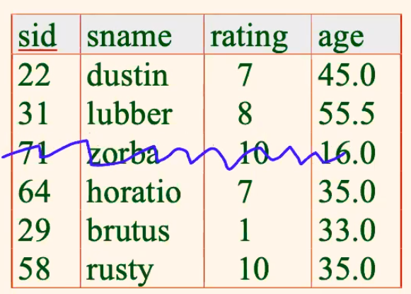
SELECT S.rating, MIN(S.age)

notice that the aggregate operators are not evaluated at this point
GROUP BY S.rating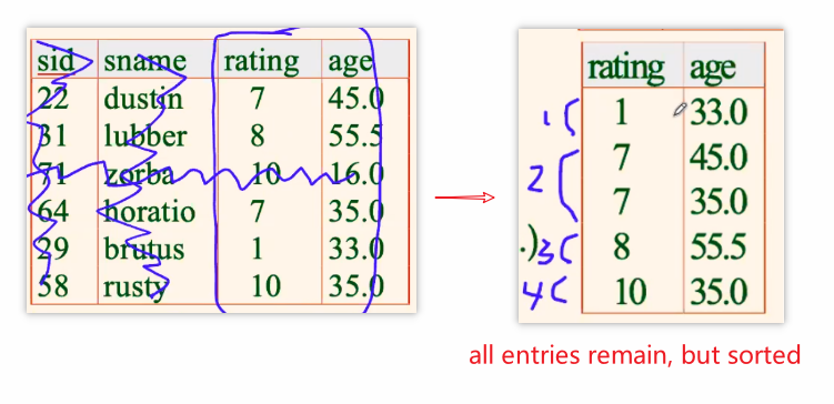
HAVING COUNT(*) > 1 which eliminates by GROUPS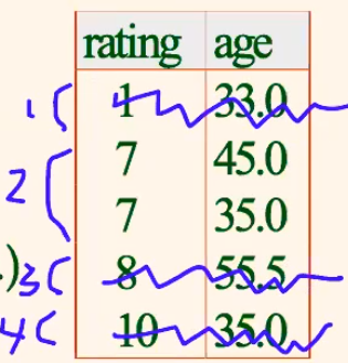
(Book-keeping) the aggregate operator is executed ` MIN(S.age)`:

For Example:

Task: For each red boat, print the bid and the number of reservations for this boat

Solution:

SELECT	B.bid,  COUNT(*) AS num_of_reservations
FROM	Boats B, Reserves R
WHERE	R.bid=B.bid AND B.color=‘red’
GROUP BY  B.bid

Alternatively:

SELECT	B.bid,  COUNT(*) AS num_of_reservations
FROM	Boats B, Reserves R
WHERE	R.bid=B.bid
GROUP BY  B.bid, B.color
HAVING	B.color='red'

which does:

GROUP BY B.bid, B.color first, and then filter it using HAVING

Group By With Correlated Queries

Reminder:

HAVING uses group qualification, which is basically qualification expression evaluated inside EACH GROUP

such as the average age of sailors in each group must be > 25

For Example:

Task: Find the age of the youngest sailor with age > 18, for each rating with at least 2 sailors (of any age)

Solution:

SELECT	S.rating,  MIN(S.age)
FROM	Sailors S
WHERE	S.age > 18
GROUP BY  S.rating
HAVING	1  <  (SELECT	COUNT (*)
               FROM		Sailors S2
               WHERE	S.rating=S2.rating)

where we have to use nested correlated SQL queries:

SELECT	S.rating,  MIN(S.age)
FROM	Sailors S
WHERE	S.age > 18
GROUP BY  S.rating
HAVING	"FOR EACH GROUP, 1  <  (SELECT	COUNT (*)
                               FROM		Sailors S2
                               WHERE	S.rating_of_each_group =S2.rating)"

Alternatively:

SELECT	S.rating,  MIN (S.age)
FROM	Sailors S, (SELECT rating 
                    FROM Sailors
                    GROUP BY rating
                    HAVING COUNT(*) >= 2) ValidRatings
WHERE	S.rating=ValidRatings.rating AND S.age > 18
GROUP BY	S.rating

where you are basically:

computing ratings with at least 2 sailors first
filtering the ages to $>$ 18
group them by each rating, and find minimum

Null Values

Basically, since we have NULL values in SQL, we need to do logical comparisons with 3-values.

AND

	T	F	N
T	T	F	N
F	F	F	F
N	N	F	N

Other Joins

Outer Joins

Outer Joins

rows included even if there is no match. This row is also indicated with Null fields

Left Outer Join

rows in the left table that do not match any row in the right table appear exactly once, with column from the right table assigned NULL values.

if there is a match, then there could be multiple values since it is just a cartesian product + selection

same as Left Join

Reminder

In the end, JOINs are just doing a cartesian product and a $\sigma$

SELECT S.sid, R.bid
FROM Sailors S LEFT OUTER JOIN Reserves R ON S.sid = R.sid

so that:

every row of the left table appears in the result
if rows from the left table did not match any in the join, then it still appears but has null
- regular join will not have this functionality

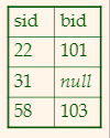
RIGHT OUTER JOIN:

the reverse

FULL OUTER JOIN:

both, left and right

Examples

Task: For each boat color, print the number of reservations for boats of that color (e.g., (red, 10), (blue, 3), (pink, 0))

Solution

SELECT B.color, COUNT(R.sid)
FROM Boats B LEFT OUTER JOIN Reserves R ON B.bid=R.bid
GROUP BY B.color

where:

remember that each boat can only have one color

Task: Print the sid and name of every sailor and the number of reservations the sailor has made.

Solution:

SELECT S.sid, S.sname, COUNT(R.bid)
FROM Sailors S LEFT OUTER JOIN Reserves R ON S.sid=R.sid
GROUP BY S.sid, S.sname

Note that

whenever you have GROUP BY some_id, no matter how many attributes you add afterwards, it will not affect the result

Task: Print the sid of every sailor and the number of different boats the sailor has reserved.

Solution

SELECT SR.sid, COUNT(DISTINCT SR.bid)
FROM (SELECT S.sid, R.bid
      FROM Sailors S LEFT OUTER JOIN Reserves R ON S.sid=R.sid) SR
GROUP BY SR.sid 

Values

Basically this is used to create a constant table

For Example:

Creates a constant table

VALUES (1, 'one'), (2, 'two'), (3, 'three')

Insert into:

INSERT INTO Sailors
VALUES (22, ‘dustin’, 7, 30)

Some trick other tricks:

CREATE VIEW TopSailors AS (
    SELECT sid, sname
    FROM Sailors 
    WHERE ratings >= 10
    UNION
    VALUES (2264, ’Alex Biliris’)
)

Building up Complicated SQL Statements

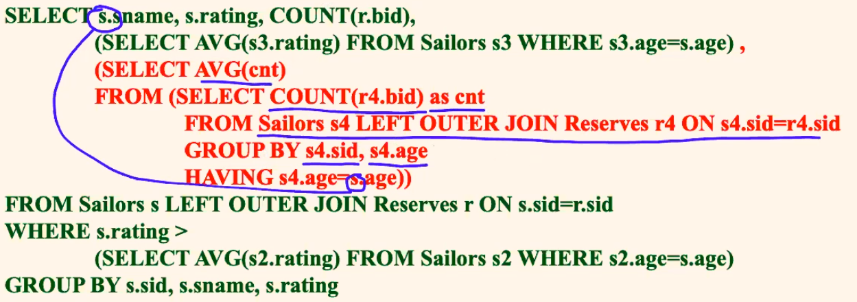
Consider the statement:

SELECT s.sname, s.rating, COUNT(r.bid),
	(SELECT AVG(s3.rating) FROM Sailors s3 WHERE s3.age=s.age) ,
	(SELECT AVG(cnt)
     FROM (SELECT COUNT(r4.bid) as cnt
           FROM Sailors s4 LEFT OUTER JOIN Reserves r4 ON s4.sid=r4.sid
           GROUP BY s4.sid, s4.age
           HAVING s4.age=s.age)) 
FROM Sailors s LEFT OUTER JOIN Reserves r ON s.sid=r.sid
WHERE s.rating> 
	(SELECT AVG(s2.rating) FROM Sailors s2 WHERE s2.age=s.age)
GROUP BY s.sid, s.sname, s.rating

To parse it, we should break it into parts

Part 1:

For each sailor with rating higher than the average rating of all sailors, print the name, rating, number of boats she has reserved

SELECT s.sname, s.rating, COUNT(r.bid)
FROM Sailors s LEFT OUTER JOIN Reserves r ON s.sid=r.sid
WHERE s.rating > 
	(SELECT AVG(s2.rating) FROM Sailors s2)
GROUP BY s.sid, s.sname, s.rating

Part 2:

For each sailor with rating higher than the average rating of all sailors of the same age, print the name, rating, number of boats she has reserved

SELECT s.sname, s.rating, COUNT(r.bid)
FROM Sailors s LEFT OUTER JOIN Reserves r ON s.sid=r.sid
WHERE s.rating > 
	(SELECT AVG(s2.rating) FROM Sailors s2 WHERE s2.age=s.age) /* added here */
GROUP BY s.sid, s.sname, s.rating

notice the correlated query:

(SELECT AVG(s2.rating) FROM Sailors s2 WHERE s2.age=s.age)

Part 3

For each sailor with rating higher than the average rating of all sailors of the same age, print the name, rating, number of boats she has reserved, and the average rating of sailors of the same age

SELECT s.sname, s.rating, COUNT(r.bid),
	(SELECT AVG(s3.rating) FROM Sailors s3 WHERE s3.age=s.age) /* A COMPUTED COLUMN */
FROM Sailors s LEFT OUTER JOIN Reserves r ON s.sid=r.sid
WHERE s.rating > 
	(SELECT AVG(s2.rating) FROM Sailors s2 WHERE s2.age=s.age)
GROUP BY s.sid, s.sname, s.rating

notice that the correlated query is now at SELECT

(SELECT AVG(s3.rating) FROM Sailors s3 WHERE s3.age=s.age) which computes the value for each matching s3.age=s.age

Part 4

For each sailor with rating higher than the average rating of all sailors of the same age, print the name, rating, number of boats she has reserved, and the average rating of sailors of the same age and average number of reserved boats by sailors of the same age

SELECT s.sname, s.rating, COUNT(r.bid),
	(SELECT AVG(s3.rating) FROM Sailors s3 WHERE s3.age=s.age) ,
	(SELECT AVG(cnt) /* added nested query */
     FROM (SELECT COUNT(r4.bid) as cnt
           FROM Sailors s4 LEFT OUTER JOIN Reserves r4 ON s4.sid=r4.sid
           GROUP BY s4.sid, s4.age
           HAVING s4.age=s.age)) 
FROM Sailors s LEFT OUTER JOIN Reserves r ON s.sid=r.sid
WHERE s.rating> 
	(SELECT AVG(s2.rating) FROM Sailors s2 WHERE s2.age=s.age)
GROUP BY s.sid, s.sname, s.rating

With - Auxiliary SQL

This is a trick so that you can give names to temporary tables AND use them!

Basically, you use a subquery, and name it:

WITH RedBoats AS (
	SELECT *
    FROM Boats WHERE color = ‘red’
),  /* comma, additional WITH query */
	RedBoatReservations AS (
    SELECT bid, COUNT(*) AS cnt
    FROM Reserves 
    WHERE bid IN (SELECT bid FROM RedBoats)
    GROUP BY bid) /* no comma, one main SQL expected */
SELECT bid FROM RedBoatReservations
WHERE cnt> (SELECT AVG(cnt) FROM RedBoatReservations)

Note

Not all systems support WITH, but this is obviously very useful since it can:

make your SQL look easier to understand

avoid repetitive queries

Security and Authorization

Basically the goal is to make sure:

Secrecy: Users should not be able to see things they are not supposed to.
- E.g., A student can’t see other students’grades.
Integrity: Users should not be able to modify things they are not supposed to.
- E.g., Only instructors can assign grades.
Availability: Users should be able to see and modify things they are allowed to.

Access Control

Access Control

Based on the concept of access rights or privileges for objects

e.g. privileges to select/update a table, etc.

this is achieved by the GRANT command

Creator of a table or a view automatically gets all privileges on it.

GRANT and Revoke

Grant Command
The command looks like:
GRANT privileges ON object TO users [WITH GRANT OPTION]
where:

privileges can be the following:

SELECT

INSERT/UPDATE (col-name)

can insert/update tuples with non-null or non-default values in this column.

DELETE

REFERENCES (col-name)

can define foreign keys (to the col-name of other tables). This is actually powerful, in that the foreign table might not be able to delete/update is there is ON DELET NO ACTION, or equivalent.

this also means that by default, you can only foreign key in our own granted access tables

ALL all privileges the issuer of GRANT has

object can be a table, a view, or an entire database

users will be the logged inusername in the DBMS

GRANT OPTION:

If a user has a privilege with the GRANT OPTION, the user can pass/propagate privilege on to other users (with or without passing on the GRANT OPTION).
However, only owner can execute CREATE, ALTER, and DROP.

For Example:

GRANT INSERT, SELECT ON Sailors TO Horatio

where Horatio can query Sailors or insert tuples into it.

GRANT DELETE ON Sailors TO Yuppy WITH GRANT OPTION

where Yuppy can delete tuples, and also authorize others to do so.

GRANT UPDATE (rating) ON Sailors TO Dustin, Yuppy

where Dustin and Yuppy can update (only) the rating field of Sailors table.

Revoke

When a privilege is revoked from X, it is also revoked from all users who got it solely from X.

Grant and Revoke on Views

Since Views have some dependencies of the underlying table:

If the creator of a view loses the SELECT privilege on an underlying table, the view is dropped
If the creator of a view loses a privilege held with the grant option on an underlying table, (s)he loses the privilege on the view as well; so do users who were granted that privilege on the view (it will cascade/propagate)!

Views and Security

Advantages of using Views

Views can be used to present necessary information (or a summary), while hiding details in underlying relation(s).

Creator of view has a privilege on the view if (s)he has at least the SELECT privilege on all underlying tables.

Together with GRANT/``REVOKE` commands, views are a very powerful access control tool.

Authorization Graph

This is how the system actually keeps track of all the authorizations.

Authorization Graph

Authorization Graph Components:

Nodes are users

Arcs/Edges are privileges passed from one user to the other

Labels are the privileges

The system starts with a “``system” node as a “user`” granting privileges.

And for all times, all edges/privileges must be reachable from the system node. If not, the unreachable privilege will be removed as well.

Cycles are possible

Role-Based Authorization

The idea is simple:

privileges are assigned to roles.
which can then be assigned to a single user or a group of users.

This means that

Roles can then be granted to users and to other roles (propagation).
Reflects how real organizations work.

Database Application Development

This section will talk about:

SQL in application code
Embedded SQL
Cursors
Dynamic SQL
Via drivers– API calls (eg, JDBC, SQLJ)
Stored procedures

The aim is to talk about: how to build an application from databases

SQL in Application Code

In general, there are two approaches:

Embed SQL in the host language (Embedded SQL, SQLJ)
- in the end, there will be a preprocessor that converts your related code to SQL statements
Create special API to call SQL commands (JDBC)
- queries using APIs

However, this might be a problem:

Impedance Mismatch

SQL relations are (multi-) sets of records, with no a priori bound on the number of records.

No such data structure exist traditionally in procedural programming languages such as C++.

(Though now: STL)

SQL supports a mechanism, called cursor, to handle this.

i.e. we are retrieving the data in steps

Embedded SQL

Approach: Embed SQL in the host language.

A preprocessor converts the SQL statements into special API calls.
Then a regular compiler is used to compile the code.

Language constructs:

Connecting to a database:
```
EXEC SQL CONNECT
```
Declaring variables
```
EXEC SQL BEGIN (END) DECLARE SECTION
```
Statements
```
EXEC SQL Statement
```

For Example: C Application Code

EXEC SQL BEGIN DECLARE SECTION
char c_sname[20];
long c_sid;
short c_rating;
float c_age;
EXEC SQL END DECLARE SECTION

so that the SQL interpreter/convertor knows that:

the following variables

char c_sname[20];
long c_sid;
short c_rating;
float c_age;

can be used in queries

Then, you can do:

EXEC SQL SELECT
SELECT S.name, S.age INTO :c_sname, :c_age
FROM Sailors S
WHERE S.Sid = :c_sid

where the INTO keywords stores the queried data into host/code variables.

Note

For C, there are two special “error” variables:

SQLCODE (long, is negative if an error has occurred)

SQLSTATE (char[6], predefined codes for common errors)

However, a problem is that you sometimes don’t know how many queried data will be returned

therefore, you need Cursors

Cursor

The idea is simple:

Declare a cursor on a relation or query statement
Open/Call that cursor, and repeatedly fetch a tuple then move the cursor, until all tuples have been retrieved.
- basically, you will have an iterator
- Can also modify/delete tuple pointed to by a cursor.

For Example

Cursor that gets names of sailors who’ve reserved a red boat, in alphabetical order

EXEC SQL DECLARE sinfo CURSOR FOR
    SELECT S.sname
    FROM Sailors S, Boats B, Reserves R
    WHERE S.sid = R.sid AND R.bid = B.bid AND B.color='red'
    ORDER BY S.sname
/* some other code */
EXEC SQL CLOSE sinfo

In terms of full code:

char SQLSTATE[6];

EXEC SQL BEGIN DECLARE SECTION
	char c_sname[20];
	short c_minrating;
	float c_age;
EXEC SQL END DECLARE SECTION

c_minrating = random();

EXEC SQL DECLARE sinfo CURSOR FOR
    SELECT S.sname, S.age
    FROM Sailors S
    WHERE S.rating > :c_minrating
    ORDER BY S.sname
do{
    EXEC SQL FETCH sinfo INTO :c_sname, :c_age, /* does the data iteration */
    printf("%s is %d years old\n", c_sname, c_age);
} while (SQLSTATE != '02000');
EXEC SQL CLOSE sinfo

where:

SQLSTATE == '02000' means the end of input/cursor

Dynamic SQL

The idea is that:

the SQL query strings are now dynamic in compile time, based on some of your coding logic
an example would be the MyBatis dynamic SQL I used in Spring Boot Projects

Drivers and Database APIs

This is the other approach of using Drivers/APIs

Rather than modify compiler, add library with database calls (API)
Pass SQL strings from language, presents result sets in a language-friendly way (CBC, JDBC, and others)
Supposedly DBMS-neutral
- a “driver” traps the calls and translates them into DBMS-specific code, by their specific Drivers
- e.g. the code you write will be the same, but if you change your DBMS, you need to change your drivers

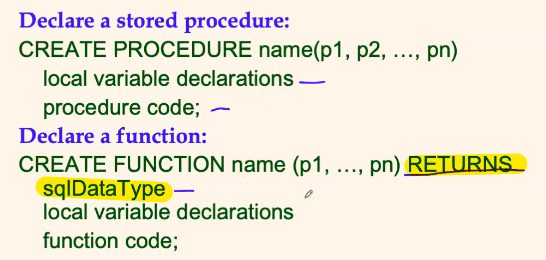
Stored Procedures

This is actually the third approach of doing this. The idea of a stored procedure is:

the application related query is stored and executed in the DBMS directly
- of course, they can still have parameters passed in from your code
therefore, this is executed in the process space of the server

For Example

First, we create and store the needed query in DBMS

CREATE PROCEDURE ShowNumReservations
	SELECT S.sid, S.sname, COUNT(*)
	FROM Sailors S, Reserves R
	WHERE S.sid = R.sid
	GROUP BY S.sid, S.sname

where this is just a plain SQL. The more interesting case would be:

CREATE PROCEDURE IncreaseRating(IN sailor_sid INTEGER, IN increase INTEGER)
    UPDATE Sailors
    	SET rating = rating + increase
    	WHERE sid = sailor_sid

where:

IN means input parameter form the caller

In general:

Stored procedures can have parameters with mode IN, OUT, INOUT

SQL/PSM

Most DBMSs allow users to write stored procedures in a simple, general-purpose language (close to SQL)

examples would be SQL/PSM standard

The syntax looks like the following:

Triggers - Server Programming

A procedure that starts automatically when a specified change occurs

Changes could be: INSERT, UPDATE, DELETE (others too)

Triggers

Think of triggers having three parts (ECA Components)

Event associated with the trigger

Condition (optional) – should it be fired?

Action – the trigger procedure/function/what should be executed

Can be attached to both tables and views

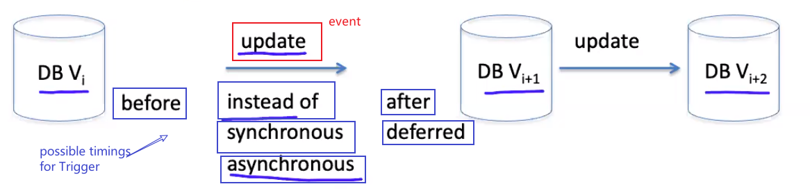
Some possible timings that you can specify for a trigger to happen is

where:

before means before the evaluation of the event

after means after

instead of means, exactly at the point when trigger condition is met, stop the execution of your program, and start trigger

synchronous means execute the trigger right after your program/event

asynchronous means execute the trigger asynchronously when the condition is met. So it does not stop the execution of your program

However, sometimes you might need to consider:

Trigger should happen at what granularity of invocation? Record (row) level or statement level?
- A row-level trigger is invoked once for each row affected by the triggering statement
- A statement-level trigger is invoked only once, regardless of the number of rows affected by the triggering statement
Hard to determine chain of events
- cascading triggers
- recursive invocation (potentially endless) of the same triggers possible
Transactional issues; trigger could be seen as
- part of the triggering statement or
- independent action
i.e. should the trigger be aborted if the transaction is aborted?

Difference between Constraints and Triggers

Constraints describe what the database’s state is (they have to be TRUE or else … )

The effects of constraints are known – no mystery if a constraint is violated (gives error)

They do not change the state of the database

Triggers are programs - very flexible mechanism

theoretically, you might not be entirely sure what happens when a trigger is executed

Order of Execution

Reminder

Triggers can be configured at many different timings

The granularity of trigger could be row level of statement level

Statement-level BEFORE triggers
- fire before the statement starts to do anything
Statement-level AFTER triggers
- fire at the very end of the statement
Row-level BEFORE triggers
- fire immediately before a row is operated on
Row-level AFTER triggers
- fire at the end of the each row operation (before statement-level AFTER triggers)
Row-level INSTEAD OF triggers (on views only)
- fire immediately as each row in the view is identified as needing to be operated on.

If more than one trigger is defined for the same event/relation

execute them In alphabetical order by trigger name!

Condition in Triggers

Reminder

Recall that a triggers having three parts (ECA Components)

Event associated with the trigger

Condition (optional) – should it be fired?

Action – the trigger procedure/function/what should be executed

Now, we want to look at what conditions can be specified

Commonly:

`WHEN Condition

If it exists, the condition needs to be true for the trigger to fire

e.g., WHEN time-of-day() > 9:30:05

Only for row-level AFTER triggers, the trigger’s condition can examine the values of the columns of

the OLD row (before an UPDATE or DELET)

and the NEW row (after an UPDATE or DELET)

in order words, you can use the parameters old and new:

e.g. WHEN new.salary > 10*old.salary.

Examples of Triggers

Syntax:

CREATE TRIGGER name 
	[BEFORE | AFTER | INSTEAD OF ] event_list ON table 
	[WHEN trigger_qualifications] 
	[FOR EACH ROW procedure | 
     FOR EACH STATEMENT procedure ] 

where:

Event -> event_list ON table
- activates the trigger
Condition -> WHEN trigger_qualifications
- should it be fired?
Action -> [FOR EACH ROW procedure | FOR EACH STATEMENT procedure ]
- the actual procedure to run

Then some examples would be:

For Example

CREATE TRIGGER init_count BEFORE INSERT ON Students 
	DECLARE count INTEGER; /* like a GLOBAL VARIABLE */
	BEGIN 
		count := 0 
	END 

where:

the Event is BEFORE INSERT ON Students

the Action is:

DECLARE count INTEGER; 
BEGIN 
	count := 0 
END 

the DECLARE count INTEGER; is like a global variable declared

and then

CREATE TRIGGER incr_count AFTER INSERT ON Students
	WHEN (NEW.age < 18)  
	FOR EACH ROW  
	BEGIN 
		count := count + 1; 
	END

For Example

If we want to populate data into another table automatically:

CREATE TRIGGER stats AFTER INSERT ON Students 
	REFERENCING NEW TABLE Stats  /* if we want to modify/deal with other tables */
	FOR EACH STATEMENT 
	INSERT INTO Stats
    	SELECT age, AVG(gpa) 
    	FROM Students 
    	GROUP BY age 

where:

now, after you insert new data into Students, the table Stats will also be populated

Normal Forms

This section talks about Schema Refinement and Normal Forms.

The Evils of Redundancy

Redundancy is at the root of several problems associated with relational schemas:

redundant storage, insert/delete/update anomalies

Main refinement technique: decomposition (replacing ABCD with, say, AB and BCD, or ACD and ABD).

in the end, we should have tables with a single, clear functional dependency.

Functional Dependency

Functional Dependency

A functional dependency $X \to Y$ holds over relation $R$ if, for every instance $r$ of $R$:

i.e. given two tuples in $r$, if the $X$ values agree, then the $Y$ values must also agree. (X and Y are sets of attributes.). An example would be $X$ being the primary key of a table $r$

In fact, this means if $K$ is a candidate key of $R$, then $K \to R$

Note that the above notation $X → Y$ is read as:

$X$ functionally determines $Y$
or $Y$ functionally depends on $X$

For Example

Consider the schema:

Consider relation obtained from Hourly_Emps (ssn, name, lot, rating, hrly_wages, hrs_worked)

We denote this relation schema by listing the attributes: SNLRWH

This is really the set of attributes {S,N,L,R,W,H}

Then some functional dependencies include

ssn is the key: $S \to SNLRWH$
rating determines hourly_wages: $R \to W$

Note

the reverse is often not true, i.e. you might not have $W \to R$

if $R = 10 \to W =100$, and $R=11 \to W=110$

obviously, reversing does not work

For Example: Functional Dependency

Instead of having:

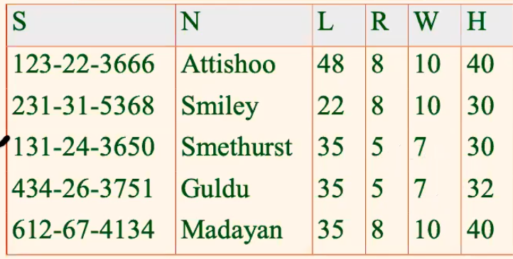
where:

$R\to W$, so that $W$ actually does not depend no $S$, but $R$!

then you have the following problem due to redundancy

Update anomaly:

Can we change $W$ in just the1st tuple of $SNLRWH$? (without messing up the mapping $R\to W$)

Insertion anomaly:

What if we want to insert an employee and don’t know the hourly wage for his rating?

Deletion anomaly:

If we delete all employees with rating $5$, we lose the information about the wage for rating $5$!

Therefore:

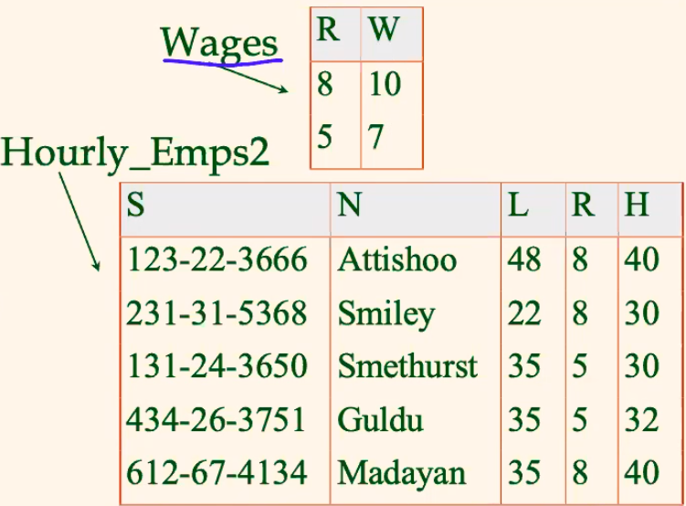
where now:

the table makes it clear that: $S \to R$, and then $R \to W$
no redundancy and clear functional dependencies

Checking Functional Decomposition

we have decomposed the schema to better forms. To check if it is correct:

perform a JOIN and see if the table matches the original one

the two tables solution means that it must be

$S \to R$

$R \to W$

hence two tables. But if $R \text{ and } H\to W$, then the above design would not work

Properties of Functional Dependency

Some obvious ones are

Armstrong’s Axioms

Armstrong’s Axioms (X, Y, Z are sets of attributes):

Reflexivity: If $Y \subseteq X$, then $X \to Y$

e.g. $Y = BC, X=ABC$, then obviously $ABC \to BC$

Augmentation: If $X \to Y$, then $XZ \to YZ$ for any Z

(Note: the opposite is not true!)

Transitivity: If $X \to Y$ and $Y \to Z$, then $X \to Z$

Following from the axioms are:

Union: If $X \to Y$ and $X \to Z$, then $X \to YZ$

Decomposition: If $X \to YZ$, then $X \to Y$ and $X \to Z$

Closure Property

the set of all FDs are closed.

recall that closure means if $F$ is the set of FDs, and I apply functional dependencies on the elements of the set, am I still inside $F$? (not getting anything new).

e.g. $F = {A \to B, B \to C, C D \to E }$ , can you cannot get $A\to E$. Otherwise it is not closed.

proof see page 9-10 of PPT

For Example

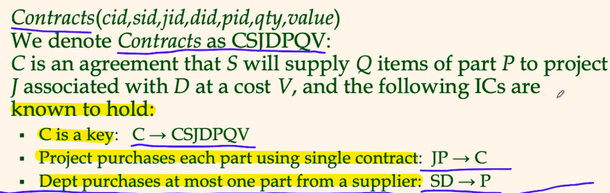
Then, this means that:

$JP \to CSJDPQV$
- because $JP \to C$, $C \to CSJDPQV$ using transitivity
and then $SDJ \to JP$
- because $SD \to P$, using augmentation
and hence that $SDJ \to CSJDPQV$
- because $SDJ \to JP$, $JP \to CSJDPQV$

So I get two primary keys

$JP \to CSJDPQV$
$SDJ \to CSJDPQV$

For Example: Closure

Consider:

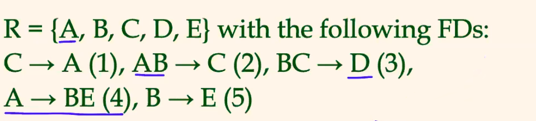
then we can get: $$

F_A^+ = { A \to A, A\to BE, A\to ABCDE}

\[where: - $A \to ABCDE$ is derived from the given FDs in the set $R$, since - $A \to ABE$ is clear, - **then using** $(2)$, means $A \to ABCE$, - **then using** $(3)$, means $A \to ABCDE$ ## Boyce-Codd Normal Form > **Why Normal Forms** > > - If a relation is in a certain normal form (BCNF, 3NF etc.), it is known that certain kinds of problems are avoided/minimized. > **BCNF** > > - relation $R$ is in BCNF if, for all $X\to A$ in the close of $F$ (i.e. $F^+$) > - $A \in X$ (called a trivial FD), > - or $X$ contains a *key* for R (i.e., X is a superkey) > > - In other words, R is in BCNF if the **only non-trivial FDs** that hold over R are **key constraints**. > - i.e. only dependencies are the *single primary key* ## Third Normal Form This basically is the most used form for designing database. - though there are still some *redundancy* > **Third Normal Form** > > - Relation $R$ with FDs $F$ is in 3NF if, for all $X \to A$ in $F^+$ > - $A \in X$ (called a trivial FD), > - $X$ contains a *key* for R (i.e., X is a superkey) > - **$A$ is part of some key for $R$.** note that: - obviously if $R$ is in BCNF, it is also in 3NF. ## Problems with Decomposition > **Three Problems with Decomposition** > > 1. Some queries become more *expensive*. > 2. **Lossless-join**: > - Given instances of the decomposed relations, we may not be able to *reconstruct the corresponding instance* of the original relation! > 3. **Dependency preserving**: > - Checking some dependencies may require joining the instances of the decomposed relations. note that: - 3NF does not have those problems, but BCNF will - but 3NF might be redundant, yet BCNF will not ### Lossless Join Decomposition > **Lossless Join** > > - Decomposition of $R$ into $X$ and $Y$ is lossless-join w.r.t. a set of FDs $F$ if, for *every instance $r$ that satisfies $F$*: > - $\pi_x(r) \bowtie \pi_y(r) = r$ > - i.e. we can reconstruct $r$ if decomposed in $X,Y$ *For Example* The following decomposition is *not lossless* 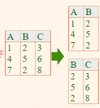![](/lectures/images/2021-04-22-COMS4111_Intro_to_Databases/Snipaste_2021-03-20_12-34-07.png) since joining back gives 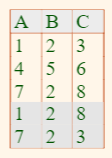![](/lectures/images/2021-04-22-COMS4111_Intro_to_Databases/Snipaste_2021-03-20_12-34-37.png) ### Dependency Preserving Decomposition > **Dependency Preserving** > > - (Intuitive) If $R$ is decomposed into $X$, $Y$ and $Z$, and we enforce the FDs that hold on X, on Y and on Z, then all FDs that were given to hold on R must also hold > - i.e. if $R$ has FDs of $F^+$, then it must be that the union $F_X^+ \cup F_Y^+ \cup F_Z^+ = F^+$, so that functional dependencies are not *lost* *For Example* - relation $ABC$, with functional dependencies $A \to B, B\to C, C\to A$ If we have decomposed into - $AB$, $BC$ then we see that the functional dependency: - $C \to A$ *is not preserved* # Object Relational DBMS First, let us look at Object Oriented vs Relational <img src="/lectures/images/2021-04-22-COMS4111_Intro_to_Databases/Snipaste_2021-03-20_12-59-10.png" style="zoom: 67%;" /> so that most of them is not there. Now, the **implemented Object-Relational DBMS** have <img src="/lectures/images/2021-04-22-COMS4111_Intro_to_Databases/Snipaste_2021-03-20_13-00-30.png" style="zoom:67%;" /> *For Example* In ORDBMS, then Schema **may** look like this <img src="/lectures/images/2021-04-22-COMS4111_Intro_to_Databases/Snipaste_2021-03-20_13-02-03.png" style="zoom: 33%;" /> and the SQL **may** look like: <img src="/lectures/images/2021-04-22-COMS4111_Intro_to_Databases/Snipaste_2021-03-20_13-05-50.png" style="zoom:33%;" /> where the new functionalities would be: - **User-defined functions** (e.g., sunset) and operators (e.g., |20|) - **Composite data types** (e.g., document, point) - **Performance**: a query optimizer aware of “expensive functions” like sunset ## ORDBMS DDL Statements Most straightforward by an example: <img src="/lectures/images/2021-04-22-COMS4111_Intro_to_Databases/Snipaste_2021-03-20_13-20-52.png" style="zoom: 67%;" /> where: - `REF IS SYSTEM GENERATED` means that you want the *system to generate reference ids*, so that you can "dereference" it and *find the object* - `CREATE TABLE Theaters OF theater_t REF is tid SYSTEM GENERATED ` means the table *contains rows of `theater_t`*, and the reference (column) of each object is called `tid`, which is `SYSTEM GENERATED` - `CREATE TABLE Nowshowing (film integer, theater ref(theater_t) SCOPE Theaters,...) ` means that - `theater ref(theater_t)` means a column `theater` *contains a pointer/reference to ANY object of type `theater_t`* - `theater ref(theater_t) SCOPE Theaters` means that column can **only point** to `theater_t` objects in the table `Theaters` - ` stars VARCHAR(25) ARRAY [10], ` means an array of size 10 containing `VARCHAR(25)` - then accessing the first name would be of table `File f` by `f.stars[0]` in a query ## Inheritance > **Note** > > - in the end, the ORDBMS combines: > - the *structuring* idea from Objected-Oriented > - the actual queries/storage from the relational DBMS > - so that in the end, everything is *still about tables/sets* *For Example* <img src="/lectures/images/2021-04-22-COMS4111_Intro_to_Databases/Snipaste_2021-03-20_13-30-25.png" style="zoom: 67%;" /> where: - `UNDER theater_t (menu text)` means **extending**`theater_t` type, and *adding an attribute* `menu` of type `text` - this is structure inheritance - `CREATE TABLE Theater_Cafes ... UNDER Theaters` means the table `Theater_Cafes` is a **subset** of the table `Theaters` - hence, by default, queries over `Theaters` are **also evaluated over `Theater_cafes`** (and all other potential subclasses at the time of evaluation) - if you don't want to do that, you can use `ONLY` # Storage and Indexing This section is about **performance**. First, we need to understand how this is stored. > **Main memory (RAM)** –while fast > > - It is volatile –we lose data between runs > - 100x more expensive than HD, 20x than SSD > > **Solid state drive (SSD, flash)** > > - Limit max capacity (2-4TB?) > - faster than HD, more durable than HD, no noise **Typical storage hierarchy**: 1. Main memory (RAM) for currently used data. 2. (Solid state, not widely used yet but it will soon) 3. Disks for the main database (secondary storage). 4. (In the past) Tapes for archiving older versions of the data (tertiary storage); not used for the operational part of the DB. ## Hard Disk > **Components of a Disk** > > <img src="/lectures/images/2021-04-22-COMS4111_Intro_to_Databases/Snipaste_2021-03-27_11-45-52.png" style="zoom:50%;" /> > > where: > > - **read/write head** writes and reads data from platters > - only one of the heads will read/write at any time > - the *smallest unit of reading is a Block size* - a multiple of sector size (which is fixed). > - **platters** spin (e.g. at 90rps) > - **arm assembly** is moved in or out to position a head on a desired track. Tracks under heads make a cylinder(imaginary!). Now, for **software** such as DBMS, (e.g. Oracle), we use a **page** as the minimal unit of data access > *Reminder* > > - A **page** is a multiple of disk blocks – the page size is determined by the DBMS or any other software using disks e.g. OS. > - Examples: 4K, 8K, 16K. > - *READ*: transfer data (a number of *disk blocks*) from disk *to main memory (RAM).* > - *WRITE*: transfer data (a number of *disk blocks*) from RAM *to disk.* > - Both are **high-cost operations**, relative to in-memory operations, so must be planned carefully! We care about this because: - Unlike RAM, time to retrieve a disk page varies **depending** upon **location** on **disk**. - Therefore, relative placement of pages on disk has **major impact on DBMS performance!** ### Accessing a Disk Page > **Time to Access a Disk Block** > > - Time to access (read/write) a disk block: > 1. **seek time** (moving arms to position disk head on track) + > 2. **rotational delay** (waiting for block to rotate under head) + > 3. **transfer time** (actually moving data to/from disk surface) **Seek time** and rotational delay **dominate**. - **Seek time** varies from about 1 to 20msec - Rotational delay varies from 0 to 10msec - Transfer rate is about 1msec per 4KB page So we want to optimize for **performance**, so we want to: - if possible, attempt to *reduce seek time* - **reduce number of disk access `I/O`** *For Example* > Usually, we assuming that a **page in OS** correspond to **continuous blocks in disk** If we want to read *one page* of`page_id=1` in **one request/system call** - the # disk access would be 1 If we want to read *8 pages* starting from `page_id=5` in **one request/system call** - still 1 disk access, since data is **contiguous** If we want to read *8 pages* starting from `page_id=5` in **eight request/system calls** - then 8 disk accesses If we want to read the entire database in **one request/system call** - then there will be **many disk accesses**, since the database is of course not an entire, consecutive pages in the hard disk --- > **Note** > > - For a sequential scan, pre-fetching several pages at a time is a big win! ## Disk Space Management **Lowest layer** of DBMS software **manages space on disk**. **Higher levels** call upon this layer to: - `allocate(int n)`: **allocate** `n` pages, return the page id of the first page of the sequence of `n` pages - i.e. `allocate(8)` would give you the first page of *eight consecutive pages*, yet `8*allocate(1)` would *not be guaranteed* to give you eight consecutive pages - `deallocate(int pid, int n)`: **free** `n` consecutive pages starting at page id `pid` Additionally, there is of course a **"page cache"**: <img src="/lectures/images/2021-04-22-COMS4111_Intro_to_Databases/Snipaste_2021-03-27_13-05-32.png" style="zoom: 80%;" /> where: - database uses its own "page cache", though the idea is the same - it is not using the OS's page cache, in order for *portability and compatibility* on different devices - additionally, if we implement this on a *database level*, we can also: - **pin** a page in buffer pool, **force a page** to disk (important for implementing CC & recovery) - **adjust replacement policy**, and pre-fetch pages based on access patterns in typical DB operations ### Page Formats: Variable Length Records This is how the DMBS manages its actual data in pages: <img src="/lectures/images/2021-04-22-COMS4111_Intro_to_Databases/Snipaste_2021-03-27_13-25-16.png" style="zoom:50%;" /> where there are **three approach** *identify* memory with a database record. When a new database record is inserted 1. a **new logical id** will be created (which maps to the physical address), then the id is the *logical id* - so to find the actual data, you need to do **two things**, translate the mapping and access the address - however, this is **more flexible** since if you moved the data, you only need to change the *mapping* 2. the id of the record will be the *physical address* - to find the actual data, you just need to do **one thing** - however, this is **less flexible** (as id cannot change) if you have moved some data 3. the id is a **combination of the actual page id and a slot number** (basically an offset) - this is the **diagram in the above**, you use `rid` for id - then, you have **both the physical address of page**, but also **flexibility WITHIN the page** (i.e. you can change the offset/slot number) ### Files of Records Page or block is OK when doing I/O, but **higher levels** of DBMS operate on **records**, and **files of records.** > **File:** > > - A *collection of pages*, each containing a collection of records. > - Must support the ability to: > - insert/delete/modify record > - read a particular record (specified using record id) > - *scan* all records (possibly with some conditions on the records to be retrieved) > - e.g. `select ... from ...` Then, the questions comes down to how the DMBS: - **stores files of records** (i.e. collection of pages that contains your data) in the memory ### Unordered (Heap) File As **file** grows and shrinks, disk pages are allocated and de-allocated. To support record level operations, we must: - keep track of the pages in a file - keep track of free space on pages - keep track of the records on a page (e.g. via `rid`) *Example: Heap File Implemented as List* <img src="/lectures/images/2021-04-22-COMS4111_Intro_to_Databases/Snipaste_2021-03-27_13-35-01.png" style="zoom:50%;" /> --- *Example:* <img src="/lectures/images/2021-04-22-COMS4111_Intro_to_Databases/Snipaste_2021-03-27_13-40-25.png" style="zoom:67%;" /> --- > **Note** > > - In both of the above implementation, finding a *specific page* requires **$O(N)$ Disk Accesses**, where $N=\text{number of pages of the file/a header}$ ## Index File > **Search Key** > > - It has nothing to do with a primary key/any key in a table > - It is the **key that DBMS can then use to perform search faster** > - e.g. you want to look up students with `gpa>3.0`, then you should build an **index with search key =`gpa`** > - Any subset of the fields of a relation can built to be the search key for an index on the relation. > **Index** > > - An **index** on a file speeds up selections **on the search key fields** for the index. > - An index contains a collection of **data entries**, and supports efficient retrieval of **all data entries `k*`** with a **given key value `k`.** > - for example, `k=3.0` could have data entry `k*` which contains *all records of student with `gpa=3.0=k`* *For Example* If you want find *all students with `gpa>3.0`*, then 1. build an index on the search key = `gpa` 2. do a binary search (assuming index is sorted) 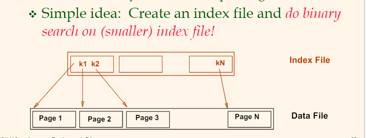![](/lectures/images/2021-04-22-COMS4111_Intro_to_Databases/Snipaste_2021-03-27_14-02-20.png) where now the **search operation will be $O(log(N))$ of Disk Accesses!** ### Hash-Based Indexing <img src="/lectures/images/2021-04-22-COMS4111_Intro_to_Databases/Snipaste_2021-03-27_14-09-49.png" style="zoom:50%;" /> where: - we have a hash function $h(k)$, which takes a parameter $k=key$:\]

h(k) \text{ mod } N

\[- then the Disk Access is in $O(M)$ for **look ups**, where $M$ is the **number of overflow pages in a bucket** - in general, this will be small ($O(M) \approx 1.2$), but we can optimize anyway by: - *increase the number of buckets* - hash function that *evenly distribute the entries* > **Advantage** > > - In other words, Hash-Based indexing is *really fast for equality searches* > > **Disadvantage** > > - this is bad if we need $\le$ or $\ge$, because we have eventually *lost the $key$ information into $h(k) \text{ mod } N$* > - therefore, we would need $O(N)$ again for range searches to look at *entries in every bucket* ### B+ Tree Indexes > *Reminder: Binary Tree* > > - anything on the **left** is smaller than the parent, and the **right** larger or equal to the parent > - since this *might be be balanced*, the tree could just have a really large height > **B+ Tree** > > - the idea is that each **non-leaf node contains** > > 1. a list of `(pointers, key)` to the children, where `key` is the key of that children. Also called the **index entry** > > 2. the list inside each node is **sorted** > > <img src="/lectures/images/2021-04-22-COMS4111_Intro_to_Databases/Snipaste_2021-03-27_14-52-41.png" style="zoom: 67%;" /> > > - the **leaf node contains** > > - the *actual data entry* (i.e. records/pages) > > - this tree is **balanced** > > <img src="/lectures/images/2021-04-22-COMS4111_Intro_to_Databases/Snipaste_2021-03-27_14-29-56.png" style="zoom:50%;" /> > > notice that the **leaf nodes are also connected**, so that it will be easy to implement $\ge$ or $\le$ search *For Example* <img src="/lectures/images/2021-04-22-COMS4111_Intro_to_Databases/Snipaste_2021-03-27_14-34-13.png" style="zoom: 67%;" /> where notice that: - each `p_key` in the **parent entry** point to the child node who **only contains `key < p_key`** - then the Disk Access is `O(levels)`, in **real life**, this will be $O(level) \approx 3$ (**this will be for equality look up**) - assumes that each node is of size `8K`, and each pair of `(pointer, key)` is `8B`, then we have in most cases `3` levels > **Note that** > > - the `index_entry` **only contains**: > 1. the key > 3. the pointer to next level > > It does **not** contain the data record/row > - Therefore, you can technically find information **on the last level** > > - so that Range Queries become easy > **Advantage** > > - For each **equality search**, in real life, `O(3)` **Disk Access** (i.e. how many times we need to go down) > - binary search in the list is done in *computer*, so does not count towards Disk Access > - For each $\le$, $\ge$ **search**, we would have `O(3)+O(M)`, for `M` being the actual number of entries satisfying the predicate > - e.g. if we needed `age > 24`, and there are `10` entries for that, then we have `3+10=13` Disk Accesses ### Primary and Secondary Index The above did two algorithms did not specify **how the index entry stores the data records/address of the data record** in fact, the two approaches are: 1. **Primary Index**: index entry `k*` contains the data 2. **Secondary Index** the index entry `k*` contains the `rid` of the data (i.e. the pointer to it) <img src="/lectures/images/2021-04-22-COMS4111_Intro_to_Databases/Snipaste_2021-04-02_22-35-14.png" style="zoom: 50%;" /> where: - for example, if for a entry we have `k=3`, then `data_record = [actual record of that Student with gpa=k=3]` > **Advantage for Primary Index** > > - Fast, *saves one Disk Access* as the data is already there > > **Disadvantage for Primary Index** > > - Makes the *data entries large* > **Advantage for Secondary Index** > > - Makes the *data entries small* > > **Disadvantage for Secondary Index** > > - Need *one more extra Disk Access* ## Clusters Clustering requires some **mathematical order** present in the data records > **Clustered Index** > > - If **order of data records** is the same as, or `close to’, **order of data entries**, then called clustered index. *For Example*: <img src="/lectures/images/2021-04-22-COMS4111_Intro_to_Databases/Snipaste_2021-03-27_15-22-27.png" style="zoom: 67%;" /> In general, **clustered index** would be faster, because: if I am fetching `key=pga>=3,0`, and that we **know there are $10$ data records that matches that** - having clustered index means we have `3` Data Access + **`1` System call** to fetch all the $10$ **consecutive data records** - e.g. if it happens that the 10 records are on the same page, then `1` System call = 1 Disk Access here - having un-clustered index means we have `3` Data Access + **`10` System** calls/Disk Accesses to fetch since they are **discontinuous** ## Composite Indices > **Composite Keys** > > - Composite Search Keys: Search on a **combination of fields.** > - for example if we have search key = `<sal, age>` > - then **Equality query** may look like `age=20 AND sal=75` > - **Rane query** may look like `age=20` or `age=20 AND sal > 10` > - Data entries in **sorted by search key** to support range queries. > - e.g. by Lexicographic order, or Spatial order. <img src="/lectures/images/2021-04-22-COMS4111_Intro_to_Databases/Snipaste_2021-03-27_15-29-16.png" style="zoom:50%;" /> TODO this should be data entries? Yes, should be data entries > **Note** > > - a data entry with key `<sal, age>` would be *different from* the key `<age, sal>`, where for the former, `sal` is **compared first**, and then `age` ## Performance Summary <img src="/lectures/images/2021-04-22-COMS4111_Intro_to_Databases/Snipaste_2021-03-27_15-36-53.png" style="zoom:67%;" /> remember the above is about **number of Disk Accesses** ## Index Selection Guidelines 1. Attributes in `WHERE` clause are candidates for index keys - **Exact** match condition suggests **hash** index. - **Range query** suggests **tree** index. - Clustering is especially useful for range queries; can also help on equality queries if there are many duplicates. 2. Before creating an index, must also consider the impact on updates in the workload! - Trade-off: Indexes can make queries go faster, **updates slower**. Require disk space, too. > **Note** > > - Try to choose indexes that benefit as many queries as possible. Since **only one index can be clustered per relation**, choose it based on important queries that would benefit the most from clustering. ## Index Syntax ```sql CREATE [UNIQUE] INDEX index-name ON Students (age, gpa) WITH STRUCTURE = [BTREE | HASH | ...] [WHERE <predicate>] ``` where: - `[WHERE <predicate>]` means that only if the record *matches the predicate*, it will be placed into the `INDEX` - `CREATE [UNIQUE] INDEX` means that the *entry of a key will only contain ONE record* # Query Evaluation Optimization If we want to keep **all of our data in a sorted manner**, when one storage we want to use would be: - B+ Tree with *primary index* storage (not secondary index since that would no be the storage anymore) Keeping data in some order will **help us later with query optimization** > **Query Plan** > > - how we should compute that query, e.g. in what order > **Overview of Query Evaluation** > > 1. For a given query, **what plans** are considered? > - obviously not all of them, which would take very long > 2. How is the **cost of each plan** estimated? > - the aim here is to quickly *estimate* > > **Ideally**: Want to find best plan. > > **Practically**: Avoid worst plans! Before discussing the System R Approach, lets look at something else related. Some common techniques for *evaluating relational operators* could be: > **Common Techniques of Evaluating/Computing Queries** > > - **Indexing**: if there is a `WHERE`, then we should use some sort of indexing to get the data back > - **Iteration**: sometimes, we need to scan all tuples/rows > - **Partitioning**: by sorting or hashing, we can partition the input tuples and replace an expensive operation by similar operations on smaller inputs > - i.e. breaking up the query into smaller, more efficient parts Note the above talks about how the **query itself might be evaluated** ## Statistics and Catalogs Before going to talk about optimization, we need to know **what is available for us** in the DBMS > **System Catalogs** > > This is maintained by the DMBS, and typically contain at least: > > - `# tuples` (NTuples) and `# pages` (NPages) for each relation. > - `# distinct key values` (NKeys) and NPages for each index. > - Index height, low/high key values (Low/High) for each tree index. > > Catalogs updated **periodically**. > > - Updating whenever data changes is too expensive; lots of approximation anyway, so *slight inconsistency is ok*. > - Usually meta information might not be updated timely ### System Catalogs Basically, they are **system tables** that store additional information on the relations you have. > **System Catalogs** > > For each index, it **stores**: > > - structure (e.g., B+ tree) and search key fields > > For each relation, it **stores**: > > - name, file structure (e.g., Heap file) > - attribute name and type, for each attribute > - index name, for each index > - integrity constraints > > For each view, it **stores**: > > - view name and definition > > **Plus** statistics, authorization, buffer pool size, etc. *For Example* <img src="/lectures/images/2021-04-22-COMS4111_Intro_to_Databases/Snipaste_2021-04-02_21-40-28.png" style="zoom:50%;" /> where: - `rel_name` means in *which table is the `attr_name` belonging to* - usually, those tables will also contain *data about themselves* ## Access Path > **Access Path** > > - an access path is about *how to actually retrieve tuple/rows* of a table > - e.g. should I scan through everything in the Heap, or should I index into a Hash Table? > - i.e. how to *figure out where the data is* *For Example* **(B)Tree Indexes** for with primary/secondary indexes built on a *composite search key* `<a,b,c>` - then, every time when we are querying a *prefix in the search key*, for example `WHERE a=5 AND b=3`, we **can use** it - if we are querying `WHERE a=5 AND c=3`, then this indexing **cannot be used** **Hash Index** index built on a *composite search key `<a,b,c>`* - then, the only query that we can use here is `WHERE a=5 AND b=6 AND c=7` - all the rest queries **cannot be used** --- > **Summary** > > - B+ Tree works when a `WHERE` query involve only attributes in a *prefix of the search key* > - Hash Table works when a `WHERE` query involves *every attribute in the search key* ### Conjunctive Normal Form One problem that we avoided in the example above is for *queries using `OR`* Consider: ```sql WHERE (day<8/9/94 AND rname=‘Paul’) OR bid=5 OR sid=3 ``` To "simplify" this, we can **convert it to conjunctive normal form (CNF)** - i.e. where each term is connected by `OR` only ```sql WHERE ( day<8/9/94 OR bid=5 OR sid=3 ) AND (rname=‘Paul’ OR bid=5 OR sid=3) ``` ## (Selection) Most Selective Access Path This is basically to deal with **selection $\sigma$**. Then, one idea of optimization is to find the **most selective access path** > **Most Selective Access Path** > > - An index or file scan that we estimate will require the **fewest page I/Os** > - i.e. *fewest steps to compute that* -> fewest records returned = easier to deal with later > - Terms that match this index **reduce the number of tuples retrieved**; other terms are used to discard some retrieved tuples, *For Example* If we have something generic:\]

\sigma_{T_1 \land T_2 \land T_3 \land …}(\text{Some Table})

\[where: - matching $T_1$ has only **one records** - matching $T_2$ has 100 records Then obviously we should **start with evaluating $T_1$**, which is the **most selective access path** in this case - then you might just need *only a few Disk Access to fetch records that match $T_1$,* and that's it --- > **In Summary** > > This means that we need to think about and **estimate**: > > - How **fast the $T_1$ can be evaluated** > - How **big** does the result look like **after evaluating $T_1$** ### Using an Index for Selection Consider the example: <img src="/lectures/images/2021-04-22-COMS4111_Intro_to_Databases/Snipaste_2021-04-02_22-39-14.png" style="zoom:50%;" /> where we need to find `sname` start with `A` or `B` basically 1. we go down the B Tree, e.g. the Left Most Data Record 2. Look up our System Table to know if it is a *primary/secondary index* 3. Range query *towards right* until a name starting with `C` > **Note** > > - if we don't have a B+-Tree, or the search key is *not `sname`*, then we **cannot/should not** use it for selection Now, we know what the *access path* looks like. We now need to think/estimate the **size of return values** > **Approximation for Size of Return Values** > > - For this course, the **only strategy** we will use is **assuming uniform distribution** Therefore, in this case, the *estimated size* is:\]

\frac{2}{26}=\frac{1}{13} \approx 10\% \text{ of the total number of records}

\[Then, say we have 10,000 tuples on 100 B-tree pages: - with a *clustered* index, cost is little more than 100 I/Os; - if *un-clustered*, up to 10,000 I/Os! ## Projection Optimization Now, we wan to **optimize projection** $\Pi$ *For Example*: Consider the query: ```sql SELECT R.sid, R.bid FROM Reserves R ``` The **only** way to optimize is: - if we happen to have a **Hash Table/B-Tree whose search key is `<sid, bid>`**, then I can **just look at/scan the search key** without needing to read the record - i.e. we are only *scanning through the search keys*, this is also called the **Index Only Evaluation** - Basically, this is optimization because the *number of total pages of data records in Heap* $>$ *number of total pages of search keys in Heap* Otherwise, we need to *scan the entire Heap* --- Now, what is **`distinct`** is specified? ```sql SELECT DISTINCT R.sid, R.bid FROM Reserves R ``` if we scan the entire Heap, this will be costly because: - we need to somehow figure out if each record *is duplicated*, which can be done by *sorting the records in the end*, but overall costly **One** ways to optimize is to use a *Hash Table*: 1. create a Hash Table with search key/bucket `<sid, bid>` 2. as we fetch each record from Heap, we dump it into the Hash Table 3. In the end, we just need to do a **Index Only Evaluation** on the Hash Table we created ## Join Optimization > *Reminder* > > - A join looks like $R \bowtie_{i=j} S$, and we needed to basically do a **cartesian product** like: > > ```python > for each tuple r in R: > for each tuple s in S: > if (r.i == s.j): > add <r, s> to result > ``` > > so basically the cost is huge. *For Example*: Let us have two tables $R$, and $S$, where: - $M_R$ is the *number of pages in $R$* - $M_S$ is the *number of pages in $S$* - $p$ is the *number of data records/tuples per page* Then: - the brute force no-index JOIN will need:\]

M_R + [(M_R \times p) \times(M_S \times p)]

\[since we need to 1. read in one of the entire table 2. read *one record at a time* for this algorithm for search However, since the idea is to **add the result if there is a MATCHING** from a record in table R and a (or many) record in S, we could do: - if we have a B-Tree indexing on the column of *one of the relation*\]

M_R + [(M_R \times p) \times 3]

\[- this makes sense because for each record of $R$, we just needed *$3$ Disk Access (B-Tree traversal)* to find out if there is an **equivalent** entry on $S$ - we *only needed to read the entire table $R$* ($M_R$ Disk Accesses since we read by page) in the beginning, and THEN do the search. - if we have a Hash Table indexing, then obviously:\]

M_R + [(M_R \times p) \times 1]

\[> **Note** > > - Since each record on $R$ could match *multiple records* on $S$, then clustering can *still help even if it is equality search* > - if clustered, then all records of `<i=1, j=1>` are close to each other, so fetching them is easy $\approx 1$ Disk Access > - if un-clustered, still need to look at *each `RID`*, so more Disk Accesses are needed > - Since the above provides a formula, we can **basically estimate the I/O cost using the above** ### Sort-Merge If the two tables $S$ and $R$ are *sorted*, we can do the following: 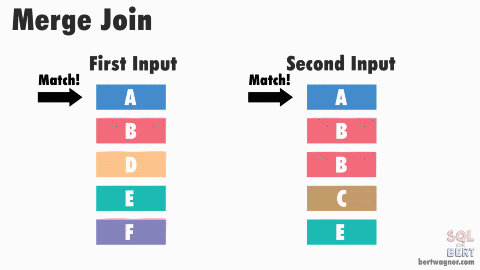![](https://bertwagner.com/wp-content/uploads/2018/12/Merge-Join-1.gif) where we have *two pointers*: - if the pointer on the Left Table is on value **smaller than** the pointer on the Right Table, move the left (increase it) **until hit** - if the pointer on the Left Table is on value **large than** the pointer on the Right Table, move the right (increase it) **until hit** Therefore, the cost is (on **average**):\]

M_S + M_R

\[since we just needed to scan the records *per page of both table*, no need to Disk I/O it per record, so cost is $M_S + M_R$ In general, if we **include the cost of sorting**\]

N\log(N) + M\log(M) + (N+M)

Worst Case Scenario

if we happen to have each row of first table matching all entries of second table, then the cost is actually: $$

M_S \times M_R

$$

but then the cost of sorting is none

In practice

We can use the approximation, since this is happening commonly in reality: $$

3 \times N + 3 \times M + (N+M)

$$

in fact, the more often case is that you have indexes built on both tables, but the tables themselves are not sorted

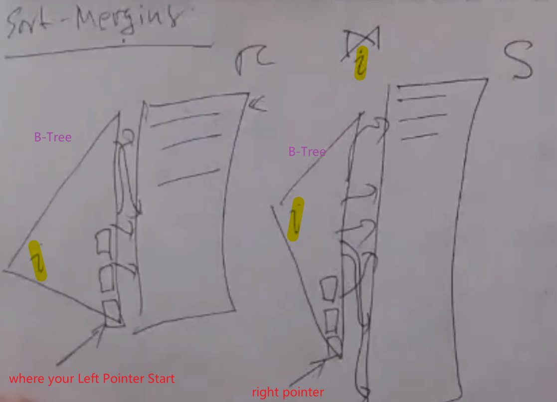
where the sorting is basically already one in the data entries, then the cost is (best case) $$

\text{total # pages of Left B-Tree’s Leaf Nodes } + \text{ total # pages of Right B-Tree’s Leaf Nodes}

Take away message

if we have some sort of index, we can always find a way to speed up the JOIN some way

Reduction Factor

Consider the query:

SELECT attribute_list
FROM relation list
WHERE term1 AND ... AND termk

Reduction Factor

Reduction factor (RF) associated with each term reflects the impact of the term in reducing result size. $$

RF_i=\frac{\text{# records matching term$_i$}}{\text{total # of records}}
\[- for example, if you have something like `WHERE id=1`, then the reduction factor is (*assuming `id` is a primary key*):\]
\frac{\text{1}}{\text{total # of records}}

$$

This means that the number of data records returned can be approximated to be $$

\text{# Result} \approx (\text{Max # Tuples}) \times \Pi_{RF}

$$ where:

$\Pi_{RF}$ means the product of all reduction factors

Implicit assumption that terms are independent

For Example

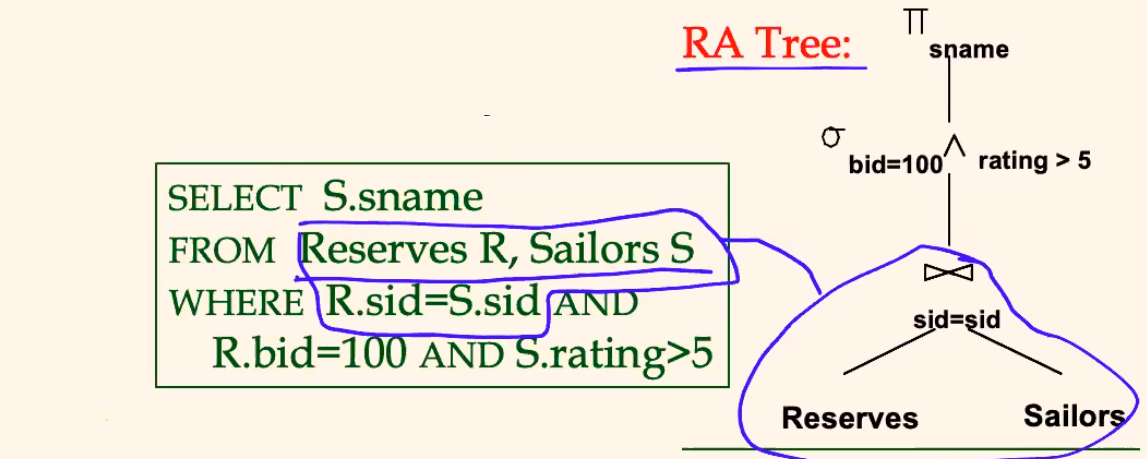
where:

technically, there could be other ways to generate the Relational Algebra Tree as well

The most straight-forward Approach would be:

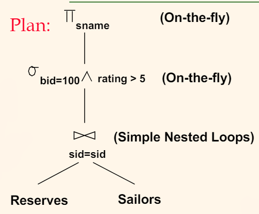
where:

“on the fly” means we are computing this while computing JOIN. Therefore, no cost

Cost: $$

\text{Cost} \approx \text{Cost of Join}

\[--- *Alternative Plan 1* <img src="/lectures/images/2021-04-22-COMS4111_Intro_to_Databases/Snipaste_2021-04-03_00-44-51.png" style="zoom:67%;" /> so we basically **decided to do $\sigma$** first **Cost**:\]

\text{Cost} \approx( \text{Cost of $\sigma_{bid=100}$} + \text{Write to $T_1$}) + ( \text{Cost of $\sigma_{rating>5}$} + \text{Write to $T_2$})+ (\text{Sort-Merge Join $T_1, T_2$})

\[basically the join would be faster --- *Alternative Plan 2 With Index* <img src="/lectures/images/2021-04-22-COMS4111_Intro_to_Databases/Snipaste_2021-04-03_00-50-32.png" style="zoom: 67%;" /> where: 1. build the Hash Table, and at the **same** time, *do the $\sigma_{bid=100}$* 2. Do the matching/`JOIN` by scanning through `Sailors` and **use the built Hash Table for look up** - at the same time, compute $\sigma_{rating>5}$ > **Note** > > - `Join` column `sid` is a **key** for `Sailors`.–At most one matching tuple. Therefore, **un-clustered index** on `sid` OK **Cost**\]

\text{Cost} \approx( \text{Cost of building Hash Table}) + ( \text{Cost of Joining with Hash Table})

\[## Summary 1. A query is evaluated by *converting it to a tree of operators* and *evaluating the operators* in the tree. 2. Two parts to optimizing a query: - Consider a set of alternative **plans**. - Must prune search space; typically, left-deep plans only. - Must estimate **cost** of each plan that is considered. - Must estimate **size** of result AND **cost** for each plan node. # Transactions A transaction is the DBMS’s abstract view of a user program: **a sequence of reads and writes** (because that all what a Database do). This is extremely useful when you are doing some sort of **concurrent execution**, or having some sort of **atomic operation** ## Atomicity of Transactions A transaction might **commit** after completing all its actions, or it could **abort** (or be aborted by the DBMS) after executing some actions. - therefore, either this thing executed completely, or none > **Atomicity of Transactions** > > - Transactions are executing **all** its actions in **one step**, or **not** executing **any actions at all** > - i.e. all in or nothing > - this is achieved by DBMS logs, which records all actions, so that it can undo/roll back the **uncommitted**/aborted transactions. (The idea is exactly the same as *journaling in OS*) *For Example:* Since the log of DBMS is basically the same idea as *journaling OS*, consider the case when: - your DBMS says you have successfully committed - data all in your Cache, not yet flushed to HDD/SSD - powered off your computer Then, technically *data is not there* even if you committed. However, the next time you boot up: - DBMS checks the log, and the **commits** to see if the Disks have it - if not, redo the committed transactions so the disk is up-to-date Therefore, it's basically the same idea as *journaling in OS*. ## ACID Properties of Transactions > **Properties of Transactions** > > - **Atomicity**: All actions in the Transactions happen, or none happen > - **Consistency**: If each Transactions is consistent, and the DB starts consistent, it ends up consistent. > - **Isolation**: Execution of one Transactions is isolated from that of other Transactions. > - even if you have *concurrent* transactions, the read/write should be still consistent > - **Durability**: If a Transactions commits, its effects persist. In reality: - the Concurrency Control Manager guarantees **C&I** - the Recovery Manager guarantees **A&D** ## Concurrency Control Consider the two transactions: ``` T1: BEGIN A=A+100, B=B-100 END T2: BEGIN A=1.06*A, B=1.06*B END ``` which *intends to* - first transaction is transferring $100 from B’s account to A’s account. - second is crediting both accounts with a 6% interest payment. If both are submitted together, i .e. concurrency, we need to make sure the **net effect** is that these two transactions running serially in some order. *For Example:* possible interleaving (i.e., a possible schedule): ```c T1: A=A+100, B=B-100 T2: A=1.06*A, B=1.06*B ``` which has the good net effect. However, the following **would not work** ```sql T1: A=A+100, B=B-100 T2: A=1.06*A, B=1.06*B ``` > In the system's point of view, this is what happens in the wrong case: > > ```sql > T1: R(A), W(A), R(B), W(B) > T2: R(A), W(A), R(B), W(B) > ``` > > basically as a sequence of read and writes. ### Scheduling Transactions A schedule is a basically a series of (scheduled) executions. > **Schedules** > > - **Serial** schedule: Schedule that does not interleave the actions of different transactions. > - simplest thing. Nothing special to do. > - **Equivalent** schedules: For any database state, the effect (on the set of objects in the database) of executing the first schedule is *identical to the effect* of executing the second schedule. > - **Serializable** schedule: A schedule that is equivalent to some serial execution of the transactions. > - A concurrent (**interleaved**) execution of two or more transactions is correct if their execution is serializable The above defined what it means to have some *correct* concurrent transactions. *For Example* Consider the case: ```c T1: a=read(x); write(x, a+4); Commit // add 4 to x T2: b=read(x); write(x, 10*b); Commit // multiply x by 10 ``` Then, we can have some possible *results*: <img src="/lectures/images/2021-04-22-COMS4111_Intro_to_Databases/Snipaste_2021-04-09_17-43-26.png" style="zoom:67%;" /> where: - the result of 1 and 2 are *serializable*, because they are **serial** (in transaction) already $\to$ both are possibly correct - thee result of 3 is *not serializable*, since the only two possible serialized result is $x=40,x=4$ $\to$ this one is incorrect ### Anomalies of Interleaved Execution Basically, this is the problem of: - if you have *simultaneous read/write to the same data* $\iff$ critical section in OS *For Example: Dirty Read* <img src="\lectures\images\typora-user-images\image-20210409175430039.png" alt="image-20210409175430039" style="zoom:67%;" /> where: - we see that the problem is $T_2$ is **reading uncommitted data**, and it has committed the value that is supposed to be **rolled back**! - again, the central cause is that those **transactions are NOT atomic WHEN concurrent** (reminder: think about the `lock`s in OS) --- *For Example: Read-Write Conflicts* <img src="/lectures/images/2021-04-22-COMS4111_Intro_to_Databases/Snipaste_2021-04-09_18-06-42.png" style="zoom: 67%;" /> where: - basically, the problem of isolation. - in short, it is the same problem of $T_1$ accessing some data and $T_2$ changing it without any sort of locks --- *For Example: Overwriting Uncommitted Data* <img src="/lectures/images/2021-04-22-COMS4111_Intro_to_Databases/Snipaste_2021-04-09_18-08-22.png" style="zoom: 67%;" /> where: - again, same problem of two transactions accessing the same data at the same time without locks ### Conflicting Operations From the above examples, we can conclude what are some **conflicted/critical operations**. > **Conflicting Operations** > > - Two operations conflict if it **matters** in which **order** they are performed. > **Read/Write Conflicts** > > - `R(x)`: conflicts with `W(x)` > - e.g. [Read-Write Conflicts] $T_1$ does read to `x`, $T_2$ does write to `x`, and $T_1$ does read to `x` > - `W(x)`: conflicts with both `R(x)` and `W(x)` > - e.g. [Dirty Read] $T_1$ does write to `x`, and $T_2$ does read to `x` > - e.g. [Overwriting] $T_1$ does a write to `x`, then $T_2$ also does a write to `x` > > All of the above are conflicts if the conflict operation of $T_2$ happened INSIDE/BEFORE $T_1$ commits Basically, only `R(x)` does not conflict with `R(x)`. ### Testing for Serializability Now, we know what could goes to conflict, we need to have a way to decide **which scheduling is serializable**. - i.e. which scheduling has the *same effect as a serialized transaction* > **Precedence Graph** > > - A directed graph in which > - **nodes** represent transactions in a schedule $S$ (T1, T2, etc) > - An edge $T_i \to T_j$, $i \neq j$, means that one of $T_i$'s operations **precedes** and **conflicts** one of $T_j$'s ops. > - A schedule $S$ is serializable if its $PG$ has **no cycles.** *For Example:*\]

S = R_1(x)R_2(x)W_1(x)W_2(x)

\[where we see that: - there are **two concurrent transactions** Drawing the PG graph, we see: <img src="/lectures/images/2021-04-22-COMS4111_Intro_to_Databases/Snipaste_2021-04-09_18-41-09.png" style="zoom: 50%;" /> where: - $T_1 \to T_2$ because $R_1(x)$ precedes $W_2(x)$ (also, $W_1(x)$ precedes $W_2(x)$) - $T_2 \to T_1$ because $R_2(x)$ precedes $W_1(x)$ There is a cycle, so this **schedule is not serializable**. > **Understanding** > > This works simply because: > > - If an edge $T_i \to T_j$ exists in the precedence graph, then, in any serial schedule $S′$ equivalent to $S$, we will have $T_i$ must appear before $T_j$. > - i.e. $T_1$ **precedes** $T_2$, this means the **net result is equivalent to $T_2$ happening after** $T_1$ > - i.e. the work that $T_2$ did **overwrites** the work of $T_1$, so net result is equivalent to $T_2$ happening serially after. > - Therefore, if you have a cycle, then it is not serializable. ### Equivalent Serial Schedule Now, if we have a *serializable schedule*, when we should be able to **do a topological sort** that produces (**one of the possible**) serialized transactions. > **Topological Sort** > > - recursively find nodes with `indegree=0` > - remove the node, and decrease all the *connected* nodes with `--indegree` *For Example:* Consider:\]

S = R_1(x)R_2(y)R_3(z)W_3(z)R_1(z)R_2(z)W_4(x)W_4(y)

$$ where we see conflicts:

$R_1(x)$ conflicts $W_4(x)$, hence $T_1 \to T_4$
$R_2(y)$ conflicts $W_4(y)$, hence $T_2 \to T_4$
$W_3(z)$ conflicts $R_1(z)$, hence $T_3 \to T_1$
$W_3(z)$ conflicts $R_2(z)$, hence $T_3 \to T_2$

So our graph looks like

graph LR
    T1 --> T4
    T2 --> T4
    T3 --> T1
    T3 --> T2

Therefore, you will have the topological sorting of:

$T_3 \to T_1 \to T_2 \to T_4$
or $T_3 \to T_2 \to T_1 \to T_4$

both of the above would be equivalent

Understanding

recall that If an edge $T_i \to T_j$ exists in the precedence graph, then, in any serial schedule $S′$ equivalent to $S$, we will have $T_i$ must appear before $T_j$.

i.e. $T_1$ precedes $T_2$, this means the net result is equivalent to $T_2$ happening serially after $T_1$

i.e. the work that $T_2$ did overwrites the work of $T_1$, so net result is equivalent to $T_2$ happening serially after.

Therefore, if $T_i$ has indegree=0, then $T_i$ basically precedes everyone

i.e. the net equivalent serial version will have $T_1$ going first

Lock-Based Concurrency Control

This is one way of how we could implement the idea mentioned above.

Strick Two-Phase Locking Protocol

Each Transaction must obtain

a S or R (shared) lock on object before reading

i.e. R(x) followed by R(x) is ok (of different transactions)

an X or W (exclusive) lock on object before writing.

i.e. R(x) followed by W(x) is not ok (of different transactions)

i.e. W(x) followed by W(x) is not ok (of different transactions)

All locks held by a transaction are released when the transaction completes

(Non-strict) 2PL Variant: Release locks anytime, but cannot acquire locks after releasing any lock.

Therefore, we can easily generate a compatibility of locks

T1/T2	Read(x)	Write(x)
Read(x)	Compatible	Not Compatible
Write(x)	Not Compatible	Not Compatible

Advantage

Strict 2PL allows serializable schedules.

Disadvantage

(Non-strict) 2PL also allows only serializable schedules, but involves more complex abort processing

Need to deal with deadlocks

Anyway we are back to the idea from OS, where we have mutex locks. Therefore, we need to think about problems such as:

deadlocks

Deadlocks

Consider the case:

T2	T2	Comment
R(x)		Granted `R(x)` lock
	R(y)	Granted `R(y)` lock
W(y)		Blocked until `R(y)` released
	W(x)	Blocked until `R(x)` released -> Deadlock

Basically, the situation is:

 sequenceDiagram
    T1->>T2: Grabs Lock(x)
    T2->>T1: Grabs Lock(y)
    T1->T2: Lock(y) ?
    T1->T2: Lock(x) ?
    Note over T1,T2: A Deadlock

An even simpler case is:

T2	T2	Comment
R(x)		Granted `R(x)` lock
	R(x)	Granted `R(x)` lock
W(x)		Blocked until `R(x)` released
	W(x)	Blocked until `R(x)` released -> Deadlock

Reminder: Deadlocks [from OS]

A deadlock situation can arise if the following four conditions hold simultaneously in a system:

there is some form of mutual exclusion (e.g. locks for a resource)

there is some form of hold and wait (e.g. holding lock1 and waiting for lock2)

basically, you are grabbing multiple locks.

a circular wait (e.g. process $P_1$ waits for $P_2$, and $P_2$ waits for $P_1$)

in a sense, this implies rule 1 and 2 as well

no preemption (e.g. timeouts for locks)

Possible Solution for DBMS

The scheduler must abort some transactions to resolve a deadlock

the brute force solution

then restart the aborted transaction

Final

Info

Thursday, April 22 at 10:10 am (Alternative exam at 9 pm)

online, cumulative, open book/notes, and access to the internet is allowed.

90 minutes

Topics included in the exam (Deck = PowerPoint Number)

Lectures #1 to #6. Included: all topics, decks 01-, 02-, 03-, 04a- and 04b- (slides 1-19 only). These are exactly the topics covered in the midterm exam.
Lectures #7 and #8. Included: Triggers (deck 04c), Security and Authorization (deck 06), Object-Relational DBMS (deck 08); general concepts at the level of detail discussed in class. You will not be asked to write your own trigger statements or Object-Relational SQL statements. Excluded: all other topics, namely, Normalization (deck 07), and Embedded SQL, APIs are excluded.
Lectures #9 to #10. Included: Storage and indexing (deck 30) and Query processing (deck 40), at the level of detail discussed in class.
Lecture #11 to #12: Included: Transaction Processing, only the first part that deals with Concurrency Control and at the level of detail covered in class (deck 50, slides <= 16 only). Excluded: Recovery (deck 50, slides > 16) and everything in Lecture #12.

Difficulty:

Homework level.
B+-Tree would be by default level 3 for lookup

Difference between Midterm

Query optimization (indexes and storages)
Transactions

Beyond CS4111

This section is of course not included in the final

Some topics below are also discussed in 4112:

Main memory and SSDs databases
Parallel/multicore databases - more delicate on concurrencies
Distributed databases
Decentralized (peer-to-peer), blockchain
Data mining (basically statistics)
Big data, data analytics, data warehousing, decision support

Some topics discussed in 6111:

Information retrieval & databases (Web search, i.e. Google Search, web scrapers, XML)
NoSQL (became NOSQL) databases, document, graph databases, key-value
- NOSQL - not only SQL, which means it also supports programming languages for query
Column-store databases

Samples of Newer DBMS

StreamBase (streaming data, acquired by TIBCO, 2013)
MongoDB (document)
Redis(open-source, in-memory key-value)
From AWS: Aurora (RDBMS), DynamoDB(NoSQL), DocumentDB (Doc DB), ElastiCache (in-memory), Neptune (graph), QLDB (blockchain), Redshift (data warehousing), Timestream (time series)

Useful Tricks

Auto-generated column in PostgreSQL

ALTER TABLE "Piazza" ALTER COLUMN cid ADD generated always as identity (START WITH 13)

Good Queries

Setup:

student(sid, sname, sex, age, year, gpa)
dept(dname, numphds)
prof(pname, dname, FK(dname)->dept)
course(cno, cname, dname, FK(dname)->dept)
major(dname, sid, FK(dname)->dept, FK(sid)->student)
section(dname, cno, sectno, pname, FK(dname, cno)->course, FK(pname)->prof)
enroll(sid, grade, dname, cno, sectno, FK(sid)->student, FK(dname,cno,sectno)->section)

Print the name of students who have enrolled in all courses offered by the ‘Chemical Engineering’ department.

SELECT *
From Student s
WHERE NOT EXISTS(
  (SELECT c.cno, c.dname 
   FROM course c 
   WHERE c.dname='Chemical Engineering')
   EXCEPT
   (SELECT c.cno, c.dname 
    FROM course c
    JOIN enroll e on e.cno = c.cno
    WHERE s.sid = e.sid AND c.dname='Chemical Engineering') /* inner query -> nested loop */
)

Note

this can be further simplified to:

SELECT *
From Student s
WHERE NOT EXISTS(
  (SELECT c.cno, c.dname 
   FROM course c 
   WHERE c.dname='Chemical Engineering')
   EXCEPT
   (SELECT e.cno, e.dname
    FROM enroll e
    WHERE s.sid = e.sid /* AND e.dname='Chemical Engineering' */)
)

Print the name and age of the student(s) with the highest GPA in their exact age group

SELECT *
FROM student s
WHERE s.age <= 18 AND s.gpa >= ALL(
    SELECT s1.gpa
    FROM student s1
    WHERE s1.age = s.age /* inner query -> nested loop */
)

alternatively:

SELECT *
FROM student s
WHERE s.age <= 18 AND s.gpa = (
    SELECT MAX(s1.gpa)
    FROM student s1
    WHERE s1.age = s.age /* inner query -> nested loop */
)

For each department with more than 8 students majoring in the department, print the following information about the student(s) with the highest GPA within the department

SELECT *
FROM student s
JOIN major m ON s.sid = m.sid
WHERE m.dname IN ( /* For each department with more than 8 students */
    SELECT m.dname
    FROM major m
    GROUP BY m.dname
    HAVING COUNT(*) > 8) 
	AND s.gpa = ( /* highest GPA within the department */
        SELECT MAX(s1.gpa)
        FROM student s1
        JOIN major m1 ON s1.sid = m1.sid
        WHERE m1.dname = m.dname
        GROUP BY m1.dname
    )

Step 1:

get the students who are majoring in a department where there are “more than 8 students majoring in the department”

Step 2:

for each student, find the department’s corresponding MAX(GPA)

Rising stars.

We want to collect statistics about rising stars: these are students who are younger than the average age of students majoring in the same department and who have a GPA that is at least 20% higher than the average GPA of students majoring in the same department. For each department with at least 3 students majoring in the department, print the department name, the total number of students majoring in the department and the average age and average GPA of all students majoring in this department, followed by the same information for the rising stars of this department (i.e., the number of rising stars in the department as well as their average age and average GPA). Consider only those departments that have at least one rising star majoring in the department.

WITH RisingStar AS(
    SELECT *
    FROM student s
    JOIN major m ON s.sid = m.sid
    WHERE s.age  < (
        SELECT AVG(s1.age)
        FROM student s1
        JOIN major m1 ON s1.sid = m1.sid
        WHERE m1.dname = m.dname
    ) AND s.gpa >= 1.2 * (
        SELECT AVG(s1.gpa)
        FROM student s1
        JOIN major m1 ON s1.sid = m1.sid
        WHERE m1.dname = m.dname
    )
) 
SELECT m.dname, COUNT(m.dname), AVG(s.gpa) as avg_gpa, AVG(s.age) as avg_age, 
	( SELECT COUNT(*) FROM RisingStar r WHERE r.dname = m.dname) AS rs_count,  
	( SELECT AVG(gpa) FROM RisingStar r WHERE r.dname = m.dname) AS rs_gpa_avg,
FROM student s
JOIN major m on s.sid = m.sid
WHERE m.dname IN (SELECT r.dname FROM RisingStar r)
GROUP BY m.dname
HAVING COUNT(*) >= 3

where this is clear so that:

“students who are younger than the average age of students majoring in the same department and who have a GPA that is at least 20% higher than the average GPA of students majoring in the same department” is achieved by:

WITH RisingStar AS(
    SELECT *
    FROM student s
    JOIN major m ON s.sid = m.sid
    WHERE s.age  < (
        SELECT AVG(s1.age)
        FROM student s1
        JOIN major m1 ON s1.sid = m1.sid
        WHERE m1.dname = m.dname
    ) AND s.gpa >= 1.2 * (
        SELECT AVG(s1.gpa)
        FROM student s1
        JOIN major m1 ON s1.sid = m1.sid
        WHERE m1.dname = m.dname
    )
) 

“For each department with at least 3 students majoring in the department, …” is achieved by the latter part of the query

Check Constraint

To enforce total participation or $\ge 1$ participation, for the Employee and WorksIn

CREATE ASSERTION EmployeesMustWorkSomewhere (
    CHECK (
        NOT EXISTS (
            SELECT ssn  
            FROM Employee 
            WHERE snn NOT IN (SELECT snn FROM WorksIn)
        )
    )
)

Function

CREATE OR REPLACE FUNCTION "xy2437"."compute_total_sub_posts"()
  RETURNS "pg_catalog"."trigger" AS $BODY$
DECLARE
    curr RECORD;
    parent RECORD;
    curr_cid int8;
    parent_cid int8;
    action_type int4; -- 0:old, 1: new
BEGIN
    raise notice 'OLD: %, NEW: %', OLD, NEW;
    raise notice 'OLD.child_cid: %, NEW.child_cid: %', OLD.child_cid, NEW.child_cid;

    -- check action that activates the trigger
    if OLD is NOT NULL then
        action_type := 0;
        curr_cid := OLD.cid;
    elsif NEW is NOT NULL then
        action_type := 1;
        curr_cid := NEW.cid;
    end if;


    SELECT * FROM "xy2437"."Piazza" pz WHERE pz.cid = curr_cid INTO curr;
    SELECT cid FROM "xy2437"."Piazza_Thread" WHERE child_cid = curr.cid INTO  parent_cid;

    -- if it is deleted, we use the parent to start with
    -- if is old:
          -- current = parent of current
    if action_type = 0 THEN
          SELECT * FROM "xy2437"."Piazza" pz WHERE pz.cid = parent_cid INTO curr;
    end if;

    -- initialization
    update "xy2437"."Piazza" set c_inode.comment_words = to_tsvector("comment") where cid=curr.cid;
    update "xy2437"."Piazza" set c_inode.likes = curr.upvote where cid=curr.cid;
    update "xy2437"."Piazza" set c_inode.dislikes = curr.downvote where cid=curr.cid;
    -- end of init

    raise notice 'curr: %', curr.cid;

    while curr is NOT NULL loop

		if action_type = 1 THEN
			update "xy2437"."Piazza" 
				set c_inode.total_sub_posts = (c_inode).total_sub_posts + 1 where cid=curr.cid;
              -- curr.c_inode.total_sub_posts++;
		elsif action_type = 0 THEN
			update "xy2437"."Piazza" 
				set c_inode.total_sub_posts = (c_inode).total_sub_posts - 1 where cid=curr.cid;
			end if;

        	-- current = parent of current
         SELECT cid FROM "xy2437"."Piazza_Thread" WHERE child_cid = curr.cid into parent_cid;
         SELECT * FROM "xy2437"."Piazza" pz WHERE pz.cid = parent_cid INTO curr;

    end loop;

RETURN NEW;
END;
$BODY$
  LANGUAGE plpgsql VOLATILE
  COST 100

where:

this function is specifically used for Trigger
OLD will refer to the data after DELETE
NEW will refer to the data after INSERT
if we are doing this for UPDATE, then both NEW and OLD will be not null

Note

the keywords are only available for the trigger with AFTER event_list ON table

Trigger

CREATE TRIGGER "total_sub_posts" 
AFTER INSERT OR DELETE ON "xy2437"."Piazza_Thread"
FOR EACH ROW
EXECUTE PROCEDURE "xy2437".;

where:

"compute_total_sub_posts"() is a function that I created in the previous section

Composite Type

CREATE TYPE "xy2437"."c_inode" AS (
  "comment_words" tsvector,
  "total_sub_posts" int4,
  "likes" int8,
  "dislikes" int8
);

where:

tsvector basically can convert a string to words as their occurrences

Note: Using Full Text Search for tsvector

basically the @@ syntax:

SELECT
	pc.nickname,
	pc.evtname,
	pc."comment",
	pc.downvote,
	pc."timestamp" 
FROM
	"Piazza_Comments" pc 
WHERE
	pc.cid IN ( SELECT cid FROM xy2437."Piazza" WHERE ( c_inode ).comment_words @@'fuck' :: tsquery )

which searches for all comments that contains the word 'fuck'