CSEE4119 Computer Networks
- Chapter 1 Basics
- Chapter 2 Application Layer
- Chapter 3 Transport Layer
- Transport Services and Protocol
- Multiplexing and Demultiplexing
- User Datagram Protocol
- Principle of Reliable Data Transfer
- TCP
- Network Assisted and Delay-Based Algorithm
- Fairness
- Evolving Transport Layer Functionality
- Chapter 4 Network Layer: Data Plane
- Chapter 5 Network Layer: Control Plane
- Chapter 6 Link Layer
- Miscellaneous
Chapter 1 Basics
The internet/networking system now evolves into including lots of applications.
Additionally:
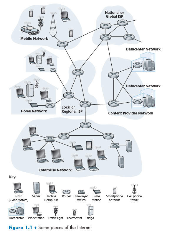
- End systems are connected together by a network of communication links (e.g. copper wire) and packet switches
Packet Switch:
A packet switch takes a packet arriving on one of its incoming communication links and forwards that packet on one of its outgoing communication links. e.g. routers and link-layer switches
It might be important to know the difference between a switch and a router.
Router:
Routers are computer networking devices that serve two primary functions:
- create and maintain a local area network
- manage the data entering and leaving the network as well as data moving inside of the network.
- has one connection to the Internet and one connection to your private local network.
Additionally,
- Routers operate at Layer 3 (Network)
- Router store IP address in the routing table
Link-Layer Switch:
A network switch is a computer networking device which connects various devices together on a single computer network. It may also be used to route information in the form of electronic data sent over networks.
So its functions are:
- store MAC address in a lookup table
- decide and forward data to the right destination, i.e. which computer
Additionally,
- Network switches operate at Layer 2 (Data Link Layer)
- Switches store MAC address in a lookup table
Last but not least:
ISP
End systems access the Internet through Internet Service Providers (ISPs), including residential ISPs such as local cable or telephone companies.
To be more detailed, it does:
- Provide a physical network connection to your device (e.g. wireless to your smart phone, or wired to your home router), supporting some basic data communication protocols (e.g. 4G, DSL, DOCSIS, Ethernet, …).
- Providing Internet Protocol (IP) connectivity, i.e. provide your device with an IP address, receive IP traffic from your device and route (send) it onto the Internet, and receive IP traffic from the Internet and route it to your device.
The Network Edge
End-system:
Devices sitting at the edge of the Internet. End systems are also referred to as hosts because they host (that is, run) application programs such as a Web browser program, a Web server program, an e-mail client program, or an e-mail server program.
- Hosts are sometimes further divided into two categories: clients and servers. Today, most of the servers from which we receive search results, e-mail, Web pages, videos and mobile app content reside in large data centers.
Access Networks
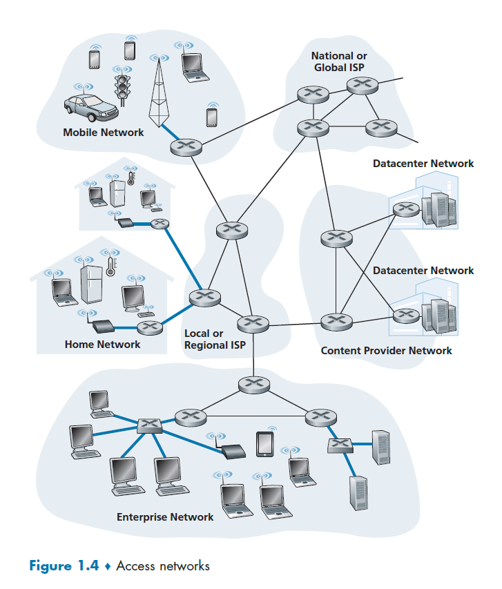
Access Network
The network that physically connects an end system to the first router (also known as the “edge router”)
Digital Subscriber Line
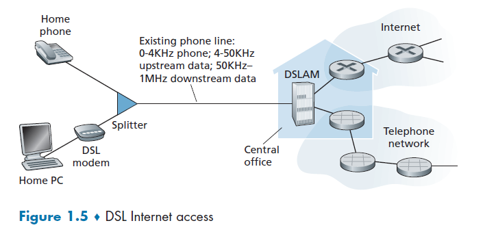
A residence typically obtains DSL Internet access from the same local telephone company (telco) that provides its wired local phone access. Thus, when DSL is used, a customer’s telco is also its ISP.
Some components used here are:
DSL Modem
DSL modem uses the existing telephone line exchange data with a digital subscriber line access multiplexer (DSLAM). The home DSL modem takes digital data and translates it to high-frequency tones for transmission over telephone wires to the CO (central office).
This means that the residential telephone line carries both data and traditional telephone signals simultaneously, which are encoded at different frequencies:
- A high-speed downstream channel, in the 50 kHz to 1 MHz band
- A medium-speed upstream channel, in the 4 kHz to 50 kHz band
- An ordinary two-way telephone channel, in the 0 to 4 kHz band
Splitter
Splitter separates the data and telephone signals arriving to the home and forwards the data signal to the DSL modem
DSLAM
DSLAM separates the data and phone signals from home and sends the data into the Internet.
Last but not least:
- this is installed particularly per user (if they have an existing telephone line).
- the DSL standards define multiple transmission rates, including downstream transmission rates of 24 Mbs and 52 Mbs, and upstream rates of 3.5 Mbps and 16 Mbps
Voice Encoding
Since essentially you want to convert a wave (your speech wave -> wave in voltage) to digital bits, you need:
- sample frequency
- number of samples
To decide the quality of your recorded voice. For example, if It captures speech in a range of 300 to 3.4 kHz, samples at 8000 samples/second with 8 bits per sample, then we have it resulting in 64 kbps of voice encoding.
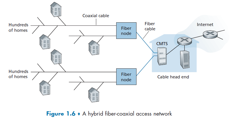
Cable Internet Access
Cable Internet access makes use of the cable television company’s existing cable television infrastructure. Therefore, A residence obtains cable Internet access from the same company that provides its cable television.
some important components here are defined below
HFS
Because both fiber and coaxial cable are employed in this system, it is often referred to as hybrid fiber coax (HFC).
Cable Modems
Cable internet access requires special modems, called cable modems. As with a DSL modem, the cable modem is typically an external device and connects to the home PC through an Ethernet port.
CMTS
At the cable head end, the cable modem termination system (CMTS) serves a similar function as the DSL network’s DSLAM—turning the analog signal sent from the cable modems in many downstream homes back into digital format.
However, the larger difference here is that:
- it is a shared broadcast medium. In particular, every packet sent by the head end travels downstream on every link to every home and every packet sent by a home travels on the upstream channel to the head end. For this reason, download and upload speed are sometimes slowed due to simultaneous uses.
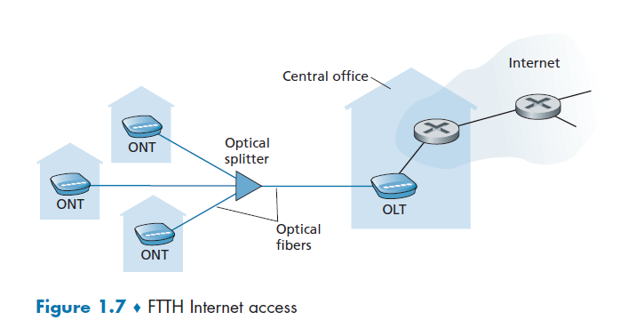
Fiber to Home
Fiber to the home (FTTH). As the name suggests, provides an optical fiber path from the CO directly to the home.
- in the DSL case, telephone line was used
- in the cable internet access case, coaxial cables were shared
where we see that
- it is split into individual customer-specific fibers until the fiber gets relatively close to the homes, but they are all fiber optics
There are two competing optical-distribution network architectures: active optical networks (AONs) and passive optical networks (PONs). AON is essentially switched Ethernet, which is discussed in Chapter 6.
PON, which is used in Verizon’s FiOS service. Figure 1.7 shows FTTH using the PON distribution architecture.
Optical Splitter
The splitter combines a number of homes (typically less than 100, as compared to the cable internet access, which typically has thousands) onto a single, shared optical fiber, which connects to an optical line terminator (OLT) in the telco’s CO
Optical Line Terminator
OLT, providing conversion between optical and electrical signals, connects to the Internet via a telco router.
Optical Network Terminator
At home, users connect a home router (typically a wireless router) to the ONT and access the Internet via this home router. This basically substitutes the role of modems in previous examples.
Ethernet and WiFi
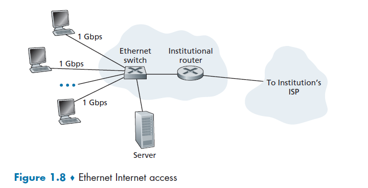
Ethernet Switch
Ethernet users use twisted-pair copper wire to connect to an Ethernet switch, and the Ethernet switch, or a network of such interconnected switches, is then in turn connected into the larger Internet.
In a wireless LAN setting, wireless users transmit/receive packets to/from an access point that is connected into the enterprise’s network (most likely using wired Ethernet), which in turn is connected to the wired Internet.
Access Point
A networking hardware device that allows other Wi-Fi devices to connect to an existing wired network. Essentially access point (base station) is just a sub-device within the LAN providing another location for devices to connect on the network.
- therefore, access point can create WLANs (Wireless Local Area Networks) while being connected to routers/switches and its functionality is limited to this only. This can be done by routers as well, e.g. embedded in a wireless router, hence you don’t require a separate AP.
Many homes combine broadband residential access (that is, cable modems or DSL) with these inexpensive wireless LAN technologies. In Figure 1.9 shows a typical home network.
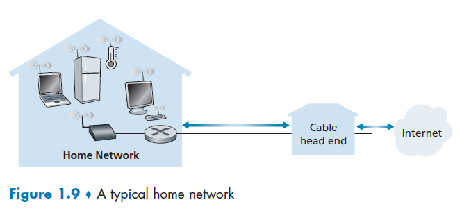
where here:
- base station (the wireless access point), which communicates with the wireless PC and other wireless devices in the home
- home router that connects the wireless access point, and any other wired home devices, to the Internet
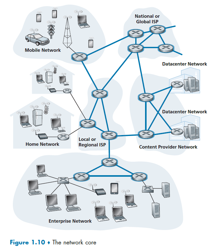
Network Core
We have covered the edges used in our network. Figure 1.10 highlights the network core with thick, shaded lines.
Performance (Delay, Loss, Throughput)
The idea is to get good performance out of switches without guarantee (of delivery). As a packet travels from one node (host or router) to the subsequent node (host or router) along this path, the packet suffers from several types of delays at each node along the path.
First, we need to know how packet loss and delay occurs.
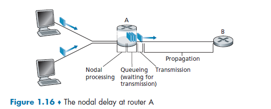
So we get:
- when the packet arrives at router A from the upstream node, router A examines the packet’s header to determine the appropriate outbound link for the packet.
- Then the packet is directed to the queue that precedes the link to router B
- then the packet has to wait on a link until there is no other packet currently being transmitted on the link
- then, it needs to push the bits of the packet onto the link
- finally, the electricity (voltage representing those bits) needs to travel towards B
- at B, we repeat the same step from 1-6
Therefore, the most important delays are
\[d_{\text{total}}=d_{\text{proc}}+d_{\text{queue}}+d_{\text{trans}}+d_{\text{prop}}\]where:
-
$d_{\text{proc}}$ is process delay, required to examine the packet’s header and determine where to direct.
- other usage include time need to check bit errors, etc.
-
$d_{\text{queue}}$ waits to be transmitted onto the link.
- Packet Queue: in general, a switch/router will have a packet queue/buffer, since it could only send one packet at a time.
-
$d_{\text{trans}}$ the amount of time required to push (that is, transmit) all of the packet’s bits into the link. Therefore, it depends on the size of information and the bandwidth
-
this can be computed by:
\[\text{transmission delay} = \frac{L}{R}\]where the length/size of the packet is $L$ bits, and the bandwidth/transmission rate of the route is $R$ bits/sec.
-
-
$d_{\text{prop}}$ time taken to transmit the data over the medium. This then depends on the distance, medium etc.
- e.g. under sea cable would have a larger $d_{\text{prop}}$, but for data centers, this would be small.
Note
- in reality, the routers keep a list of other connected router’s destination. However, the possibility of being congested in some of the router might not be recorded.
- One possible solution would be to measure latency yourself and then decide which route to send to (if you have control of it).
- Though there might be some fine changes of routes within a network, the link/route (i.e. weak tie) across networks will usually be stable.
An analogy of the above process would be:
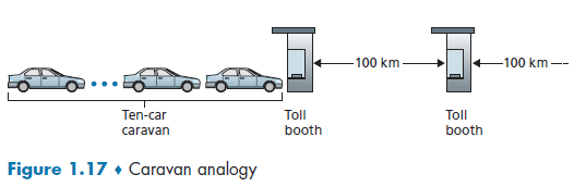
we know that:
- cars (=packet of 1 bit) contain some information
- highway segments between tollbooths (=links)
- tollbooth (=router)
Then, given that cars (=packet) propagates at speed of 100km/hour and each toll booth takes 12 seconds to service car ($d_{\text{trans}}$), we know that, for the last car (bit) to reach the destination
- each car needs to be processed/examined
- each car needs to wait for previous cars
- each car then is pushed on to the highway after 12 seconds of service ($d_{\text{trans}}$)
- each car then travels to the next tollbooth in 1 hour. $(d_{\text{prop}})$
Traceroute
traceroute in Linux:
➜ traceroute nytimes.com
traceroute to nytimes.com (151.101.1.164), 30 hops max, 60 byte packets
1  JASONXYU-NB1.mshome.net (172.27.144.1)  0.347 ms  0.326 ms  0.270 ms
2  cc-wlan-1-vlan3572-1.net.columbia.edu (209.2.216.2)  3.706 ms  3.696 ms  3.681 ms
3  cc-core-1-x-cc-wlan-1.net.columbia.edu (128.59.255.77)  3.673 ms  3.670 ms  3.627 ms
4  nyser32-gw-1-x-cc-core-1.net.columbia.edu (128.59.255.6)  3.658 ms  3.646 ms  3.640 ms
5  199.109.104.13 (199.109.104.13)  5.095 ms  5.087 ms  5.070 ms
6  nyc32-55a1-nyc32-9208.cdn.nysernet.net (199.109.107.202)  5.159 ms  3.572 ms  3.559 ms
...
where basically this is delay in a roundtrip (forth and back).
- the number in the front
1,2,3,4...means the number of TTL defined. In the above, 6 samples are tried, each with TTL 1 up to 6 respectively. - basically this shows you the hops that is needed from your end point to the destination end point, as well as the total latency.
- sometimes there are
*, which indicates that the router did not respond (e.g. configured not to respond to you) cc-wlan-1-vlan3572-1.net.columbia.eduwould be the resolved DNS/host name
Note that:
traceroutein this case would have measured all the four delays for each hop.
TTL (time to live): the number of hops in which the message should reach the destination. This is to prevent the case that your packets will go in a cycle and never reaches the destination. If the TTL gets to zero, then an error message will be sent back to the source
- For example, if the packet doesn’t reach the destination in 20 hops, just give up the packet.
- this is also added in the network layer.
- detailed implementation of
traceroutecan be found in Examples of ICMP Usages- all packets will have this field (defined by the protocol)
For Example
Consider the case when you want to debug the latency from Orlando to Seattle and vice versa.
Suppose you are at Orlando. Upon using traceroute, you see:
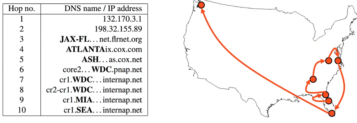
so that we have wasted some routes by going back to Florida.
Now, the problem is that routes on the internet are often asymmetric. So that going from Seattle to Orlando, we might have the path in purple:
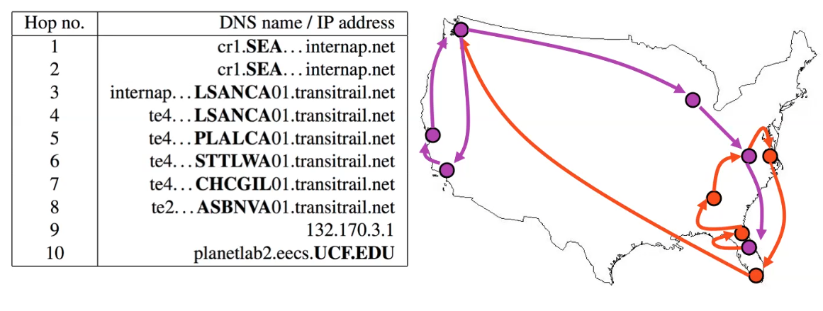
Therefore, due to the asymmetry:
traceroutefrom a reversed direction might have a different result.
Queuing Delay and Packet Loss
Queuing delay is more complicated than others. Unlike the other delays, this varies from packet to packet.
Therefore, when characterizing queuing delay, one typically uses statistical measures, such as
- average queuing delay
- variance of queuing delay
- probability that the queuing delay exceeds some specified value
Suppose, for simplicity, that all packets consist of $L$ bits, and that on average you get $a$ packets per second. Suppose your transmission rate is $R$ (being pushed off the queue to the link):
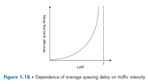
Here we notice that:
-
due to variations in packet arrival rate, when the traffic intensity is close to $1$, there will be intervals of time when the arrival rate exceeds the transmission capacity.
- on the other hand, if packets arrive exactly periodically - that is, one packet arrives every $L/R$ seconds - then every packet will arrive at an empty queue and there will be no queuing delay.
-
$La/R$ is also called the traffic intensity.
-
this is assuming there is some distribution of incoming intensity instead of a uniform one, e.g. the Poisson distribution of incoming intensity. As a result, there will be bursts of influxes at times and the queue would build up. The resulting formula would be:
\[d \propto \frac{\rho}{1-\rho}\]where:
- $\rho \equiv La/R$ is the traffic incoming intensity.
However, no loss occurs if we assumes that our router can hold infinitely number of bits. Yet this is often not true.
Packet Loss
- When a packet can arrive to find a full queue, so that there is no place to store such a packet, a router will drop that packet; that is, the packet will be lost.
- In general, the fraction of lost packets increases as the traffic intensity increases
Throughput
Throughput is different against transmission rate/bandwidth, because it is macroscopic.
Throughput
Number of bits per second that a client receives data from a host.
- therefore, it is not able between links. It is more like end-to-end measurement.
Consider the following two cases:
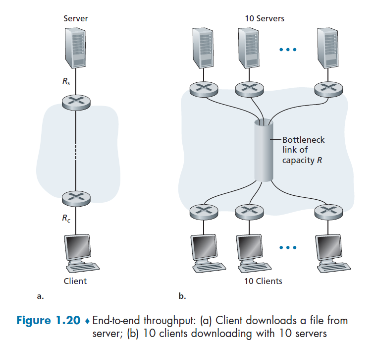
For case a), suppose we have $R_c$ for the bandwidth between router and client, and $R_s$ for the server. Then:
\[\text{Throughput} = \min\{R_c,R_s\}\]due to bottlenecks.
For case b), let all 10 serves have the same $R_s = 2$ Mbps, and all clients have $R_c=1$ Mbps. Assume the shared link is fair to every server, and it has $R=5$ Mbps. Then we have:
\[\text{Throughput} = \min{\{R_s, R/10, R\}} = 5/10 = 500 \text{ Kbps}\]Protocol Layers and Their Service Models
The entire core system of internet is very complex, since we need to organize numerous applications and protocols, various end systems and etc. To manage the complex system, we split them into manageable components (layers) and build them up.
Protocol Layering
The idea is to separating a big task into smaller tasks, and a combination of those small stacks become the protocol stack. This is needed since it needs to go though mediums such as routers, ISP, etc.
Consider the example of sending text massages from me to mom, then some challenges we need to overcome would be:
- security
- data integrity
- routing
- etc.
network designers organize protocols (tasks) - and the network hardware and software that implement the protocols - in layers. When taken together, the protocols of the various layers are called the protocol stack.
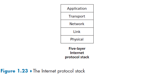
where:
- Application Layer: sending data to correct application/software
- Transport: Recovery of lost packets, congestion control, rate control
- Network: Sending packets in the right destination/direction
- Link/MAC: Getting information correctly between 2 physically connected points
- Physical: physical/science needed to send info between 2 physically connected points (i.e. how to physically transmit bit information)
Note
- in each layer, there is some protocols defining what each information received means, and what it should do next.
- in each layer, it assumes the other layer is doing their stuff correctly
Advantage
- Modularity = easier to maintain and update
Disadvantage
- One layer may duplicate lower-layer functionality. For example, many protocol stacks provide error recovery on both a per-link basis and an end-to-end basis
Analogy: Post Office
Consider the example you trying to send a recorded TV show to your friend.
Application: received the recorded disk, knows to use the TV/laptop to play it.
Transport: (e.g. error control) your friend telling you that something went wrong. e.g. you sent me the wrong episode.
Other stuff are all dealt by the post office.
Application Layer
Parsing/forming the packet in the application. So this is application specific, and only implemented in the end points as well.
Some example protocols at this level are:
- HTTP protocol (which provides for Web document request and transfer)
- SMTP (which provides for the transfer of e-mail messages)
- FTP (which provides for the transfer of files between two end systems).
Packets of information on this level will be referred to as a message.
Transport Layer
This is only implemented at end points, and adds information such as your device tells the source to repeat the information if you didn’t “hear it” clearly.
In the Internet, there are two transport protocols:
- TCP (guaranteed delivery of application-layer messages)
- UDP
Some functionalities here include:
- congestion control by having source throttles its transmission rate when the network is congested (TCP).
- breaks long messages into shorter segments
Packets of information on this level will be referred to as a segment.
Network Layer
Built upon link layer, assuming we can get a frame across two end points (via lower layers), we need to now consider where to send it. So this layer receives a frame and figures out the next hop.
- moving network-layer packets known as datagrams from one host to another.
The upper level Transport layer passes a segment (packet of information) and a destination address to the network layer (this), so we have the:
- IP protocol (which defines the fields in the datagram as well as how the end systems and routers act on these fields)
- or other routing protocols that determine the routes that datagrams take between sources and destinations
At this level, we say that data sent are datagram/packets.
Link Layer
Sending a frame, i.e. a collection of bits, over the physical layer.
Examples of link-layer protocols include:
- Ethernet
- WiFi
- cable access network DOCSIS protocol
As datagrams typically need to traverse several links to travel from source to destination, a datagram may be handled by different link-layer protocols at different links along its route.
Some link-layer protocols provide reliable delivery, from transmitting node, over one link, to receiving node, which has nothing to do with the reliability of TCP, for example, which guarantees at the application level.
Therefore, this also have additional information added to the packet.
Physical Layer
Having a medium, e.g. a copper wire, to transmit bit information across 2 physically connected points. This is the only and final place where transmission of data happened. All the above protocols are just parsing information and deciding what to do next.
Protocols at this level deal with how bits are moved between the two connected points:
- Ethernet has many physical-layer protocols: one for twisted-pair copper wire, another for coaxial cable, another for fiber, and so on.
Network Interface Card
Physical layer and data link layers are responsible for handling communication over a specific link, they are typically implemented in a network interface card (for example, Ethernet or WiFi interface cards) associated with a given link.
Encapsulation
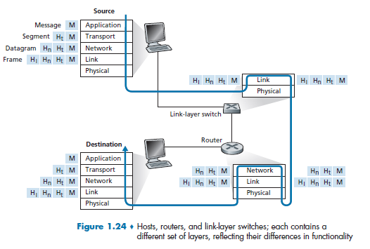
where:
-
Figure 1.24 shows the physical path that data takes
- we knew that some layers, e.g. Transport and Application, are only implemented at the end points
- what physically connects the two is the edge across physical layers. So in the end, this is the only place where data is actually transmitted.
Note
- that hosts implement all five layers, and must be identical. As otherwise a message from application of user $A$ cannot be understood by the architecture in the computer of $B$.
What actually happens when you send (origin being $A$), e.g. an email would be:
- Email application start with Application Layer forming the message, and ask the Transport Layer to deal with it
- Transport layer then takes the big package and split them into packets (if needed due to large data), and add appends additional information (so-called transport-layer header information) will be used by the receiver-side transport layer
- e.g. ensuring there is destination/source IP, destination/source MAC, packet sequence id, etc. Then, those packets are passed to Network Layer.
- The transport-layer segment thus encapsulates the application-layer message, and pass down to Network Layer
- Network Layer then appends network-layer header information to the segment, such as source and destination end system addresses, creating a network-layer datagram
- figures out where is the next hop, e.g. in the figure, which router/link-layer switch to send to.
- then pass to Link Layer
- Link Layer will add its own link-layer header information and create a link-layer frame, and pass to physical layer
- Physical layer sends the bits to the next hop, a switch in the figure
Now, at the switch:
- receives data from the Physical Layer, parse the data and move up
- parse the data in the Link Layer, recognize the Ethernet addresses and what to send to the next router, so pass down again to physical layer
- Physical Layer then send the frame by bits.
Note
- notice the need to go up and down the stack, if we need to “forward” the data to the next device.
Eventually, repeating the process will let the data reach the destination.
Protocol Stack Variants
Sometimes additional layers could be added in reality, such as:

where here we added a security layer basically.
Note
- This only works if both end-points have the same added layer. Otherwise, it would not be able to process the information correctly.
The more popular ones now is the OSI model:

where:
- this is the most common implemented model now
Chapter 2 Application Layer
In this chapter, we study the conceptual and implementation aspects of network applications.
- for example, we will learn how to create network applications via socket API
Recall that some common network apps include:
- web
- P2P file sharing
- streaming stored video (occupies the highest internet volume)
- etc.
Aim for Application Layer:
- network applications allows you to communicate between end points of different OS! So that you don’t need to write software for network-core devices (abstracted away), for example, a switch.
- i.e. you don’t need to know anything about the network layer when writing code in the application layer
Principles of Network Applications
At the core of network application development is writing programs that run on different end systems and communicate with each other over the network.
- For example, web application there are two distinct programs that communicate with each other: the browser program running in the user’s host (desktop, laptop, tablet, smartphone, and so on); and the Web server program running in the Web server host.
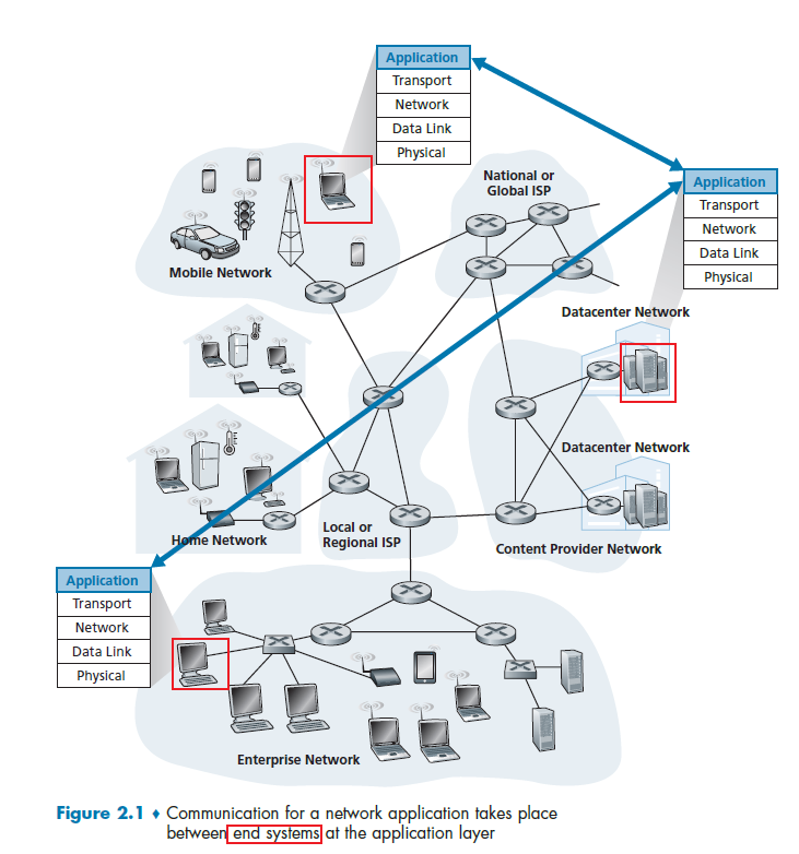
The key idea here is that your don't write and don’t need to write application programs on network-core devices (e.g. switches), as they never include application layer stuff and are already “taken care” of.
- This basic design- namely, confining application software to the end systems - as shown in Figure 2.1, has facilitated the rapid development and deployment of a vast array of network applications
Application Architecture
Again, the key idea is that, from the application developer’s perspective, the network architecture is fixed and provides a specific set of services to applications (i.e. API’s for them to work). The application architecture, on the other hand, is designed by the application developer and dictates how the application is structured over the various end systems.
Therefore, at this level, we just need to know how end-to-end devices should communicate to each other without worrying about what happens in between.
In modern application architecture (i.e. how end devices talk to other end devices), there are two predominant architecture paradigms:
- client-server architecture
- peer-to-peer (P2P) architecture.
Client-Server Architecture
A common example of network application would be a web browser which uses the following architecture
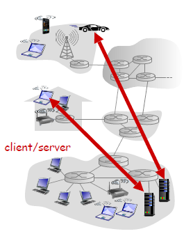
where basically you have:
- a server
- associated with some address (IP address), (e.g. whatever IP resolved from www.columbia.edu)
- always-on host
- data centers for scaling
- clients
- communicate with server. (the client initiates a connection in this case)
- but clients do not directly communicate with each other
- may have dynamic IP addresses
- essentially we move and connects to different routers, cell towers, etc.
- therefore, packets need to include the client’s IP so that the server can find it
- may be intermittently connected
- communicate with server. (the client initiates a connection in this case)
P2P Architecture
Now, there is minimal (or no) reliance on dedicated servers in data centers. Instead, we have application exploits direct communication between pairs of intermittently connected hosts, called peers.
- Basically a client, when joined this kind of network, would be that clients could be a server as well.
the motivation is so that
- resources are distributed between peers/nodes, instead of having a central server holding all the data
- so a peer connects directly with another peer
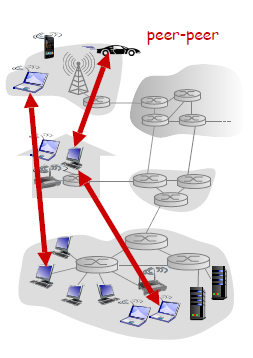
where each node/device here is:
- no always-on server, since it could be clients
- arbitrary end systems directly communicate
- both servers and clients
- peers request service from other peers, provide service in return to other peers
- self scalability – new peers bring new service capacity, as well as new service demands
- peers are intermittently connected and change IP addresses
- complex management
One example of popular P2P application is the file-sharing application BitTorrent.
For Example
You can think of the following: In a P2P file-sharing system, a file is transferred from a process in one peer to a process in another peer.
Then, this is equivalent of having:
- With P2P file sharing, the peer that is downloading the file is labeled as the client
- the peer that is uploading the file is labeled as the server.
Client vs Server
- In the context of a communication session between a pair of processes, the process that initiates the communication (that is, initially contacts the other process at the beginning of the session) is labeled as the client. The process that waits to be contacted to begin the session is the server.
Processes Communicating
In any application architecture talked about above, we basically have processes on different end points communicating over the network.
- when two processes are on the same device, inter-process communication calls (defined by OS) are used.
- when two processes are on different devices, e.g. a client and a server, then they communicate by exchanging network messages.
Interface between Process and Computer Network
So what is the abstraction of the Transport Layer when you are programming an application?
A process sends messages into, and receives messages from, the network through a software interface called a socket.
- A socket is also referred to the Application Programming Interface (API) between the application and the network
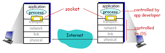
where:
- the Internet in between is the network-core devices, including routes and switches, which is abstracted away from you
The only control that the application developer has on the transport layer is (quite small)
- the choice of transport protocol
- perhaps the ability to fix a few transport-layer parameters such as maximum buffer and maximum segment sizes
Addressing Processes
To receive messages, application processes must have some identifier
To identify the receiving process, two pieces of information need to be specified:
- an IP address: the address of the host
- a port number: an identifier that specifies the receiving process in the destination host.
- identifier includes both IP address and port numbers associated with process on host.
- example port numbers HTTP server: 80 (being also a kind of permanent address)
- in reality, it is common that many different applications ends using
80, which is somewhat now like a directory management server, that tells the application which port to go
Transport Services Available to Applications
On the application layer, we might define each message’s:
- types of messages exchanged, e.g., request, response
- message syntax: what fields in messages & how fields are delineated
-
message semantics: parsing a received message
-
rules for when and how processes send & respond to messages
- open protocols:
- defined in RFCs
- allows for interoperability and discussion/emendation
- e.g., HTTP, SMTP
Recall that the socket is our current interface for Transport-Layer protocol. Since it is an API, we choose the:
- which transport protocol to use
- some parameters available for that protocol
To decide which protocol to use, we can classify each protocol along four dimesions:
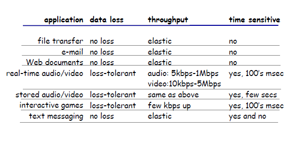
- reliable data transfer:
- if a protocol can guarantee that the data sent by one end of the application is delivered correctly and completely to the other end of the application
- so that the sending process can just pass its data into the socket and know with complete confidence that the data will arrive without errors at the receiving process
- on the other hand, you might need to have loss-tolerant applications
- throughput: the rate at which the sending process can deliver bits to the receiving process
- because network bandwidth is shared, available throughput can fluctuate with time
- natural service that a transport-layer protocol could provide, namely, guaranteed available throughput at some specified rate. So that the application could request a guaranteed throughput of $r$ bits/sec
- Applications that have throughput requirements are said to be bandwidth-sensitive applications. Many current multimedia applications are bandwidth sensitive due to encoding.
- timing
- timing guarantees can come in many shapes and forms. For example, every bit that the sender pumps into the socket arrives at the receiver’s socket no more than $100$ msec later (i.e. delay)
- for real-time applications, such as interactive games, this is very important
- security
- a transport protocol can encrypt all data transmitted by the sending process, and in the receiving host, the transport-layer protocol can decrypt the data before delivering the data to the receiving process
Recall that
- The instantaneous throughput at any instant of time is the rate (in bits/sec) at which Host B is receiving the file.
- instantaneous throughput during downloads = download speed
- If the file consists of $F$ bits and the transfer takes $T$ seconds for Host B to receive all F bits, then the average throughput of the file transfer is $F/T$ bits/sec
Note
- in general, the Applications themselves will calculate the delay and throughput of the current network by actively observing it. And in reality, the network usually does not guarantee anything. Therefore, applications needs to have some flexibility in those.
For Example
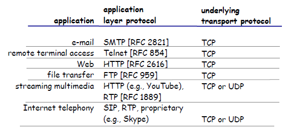
Transport Services Provided by the Internet
Up until this point, we have been considering transport services that a computer network could provide in general. Let’s now get more specific and examine the type of transport services provided by the Internet.
Some common Transport Layer Protocols would be:
- TCP: a connection-oriented service and a reliable data transfer service.
- UDP: simple and straight forward implementation
TCP Services
When an application invokes TCP as its transport protocol, you get (for free):
- Connection-oriented service: TCP has the client and server exchange transport layer control information with each other before the application-level messages begin to flow (i.e. the handshaking procedure)
- Then the connection is established, the connection is a full-duplex connection in that the two processes can send messages to each other over the connection at the same time.
- When the application finishes sending messages, it must tear down the connection
- this provides the basis for flow control and congestion control
- Reliable Data Transfer service: rely on TCP to deliver all data sent without error and in the proper order.
(Additionally, TCP also includes a congestion-control mechanism, a service for the general welfare of the Internet rather than for the direct benefit of the communicating processes.)
- throttles a sending process (client or server) when the network is congested between sender and receiver
UDP Services
UDP is a no-frills, lightweight transport protocol, providing minimal services. UDP is connectionless, so there is no handshaking before the two processes start to communicate. Therefore:
- unreliable data transfer service, so messages that do arrive at the receiving process may arrive out of order
TCP vs UDP
Below summarizes features of the two protocols.
| TCP | UDP |
|---|---|
| reliable transport between sending and receiving process | Nothing, but low overhead. |
| flow control: sender won’t overwhelm receiver | |
| congestion control: throttle sender when network overloaded | |
| connection-oriented: setup required between client and server processes (this is required for flow control or congestion control) | |
| does not provide: timing, minimum throughput guarantee, security | does not provide: reliable or in order delivery, flow control, congestion control, timing, throughput guarantee, security, or connection setup |
Note
- TCP itself does not provide security. In reality, it is usually the TLS = Transport Layer Security that provides encryption.
- In UDP, though packets might arrive out of order, you (application layer) can check and request the sender to sending again the missing packet.
So UDP might be advantageous when the data to transfer is small (e.g. DNS), or when you really need a small overhead for transfer:
Securing TCP
SSL/TLS
- provides encrypted TCP connection
- data integrity
- end-point authentication
- SSL is older, deprecated
TLS is at app layer
- apps use SSL libraries, that “talk” to TCP
- Client/server negotiate use of TLS
TLS socket API
- if you send a cleartext password into socket, it traverses Internet encrypted
Socket Programming
The goal is to learn how to build client/server applications that communicate using sockets.
Recall that there are two socket types for two transport services:
- UDP: unreliable datagram but low overhead
- TCP: reliable, byte stream-oriented
For Example
Application Example:
- client reads a line of characters (data) from its keyboard and sends data to server
- server receives the data and converts characters to uppercase
- server sends modified data to client
- client receives modified data and displays line on its screen
For UDP:
- recall that this is connectionless. Therefore, every packet needs to know its destination. As compared to TCP. which just needs to dump the packet in the established connection and you are done
- no handshaking before sending data
- sender explicitly attaches IP and port destination address for every packet
- transmitted data may be lost or received out-of-order
- (e.g. packet 1 sent on 10 MBPS link and packet 2 on 100MBPS, different routes)
- therefore, the application layer might need to anticipate and check this
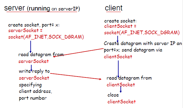
In Python, you then get for the client:
from socket import *
serverName = ‘hostname’
serverPort = 12000

# creates socket
clientSocket = socket(AF_INET, SOCK_DGRAM)
message = raw_input(’Input lowercase sentence:’)
clientSocket.sendto(message.encode(), (serverName, serverPort)) # sends to a queue

# receive a message
modifiedMessage, serverAddress = clientSocket.recvfrom(2048)
print modifiedMessage.decode()
clientSocket.close()
- notice that
clientSocket.sendto(message.encode(), (serverName, serverPort))shows that we are specifying destination for every packet
Then for the server:
from socket import *
serverPort = 12000

# create socket
serverSocket = socket(AF_INET, SOCK_DGRAM)
serverSocket.bind(('', serverPort))
print (“The server is ready to receive”)

# listening and receiving
while True:
    message, clientAddress = serverSocket.recvfrom(2048) # reads from a queue
    modifiedMessage = message.decode().upper()
    serverSocket.sendto(modifiedMessage.encode(), clientAddress)
- notice that there is only one socket
- since it is UDP, it also means that if the server if full in queue, the client will have no idea and still sends the packets (TCP would have notified the client)
UDP Takeaway
- the idea is that at every single time, there is only a one-way connection
On the other hand, when we have a TCP protocol:
- client needs to be creating TCP socket, specifying IP address, port number of server process at socket creation
- when contacted by client, server TCP creates new socket for server process to communicate with that particular client
- i.e. you
forkthat socket - allows server to talk with multiple clients
- source port numbers used to distinguish clients (more in Chap 3)
- i.e. you
Therefore, the abstraction is:
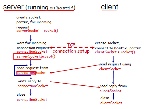
where we notice that:
- on the server, when connection is established, you will get a listening
serverSocketand aconnectionSocketwhich you would use for sending/receiving
In the client side, you get:
from socket import *
serverName = ’servername’
serverPort = 12000

# creating socket
clientSocket = socket(AF_INET, SOCK_STREAM)
clientSocket.connect((serverName,serverPort)) # server destination specified at CREATION time

# sending/receiving message
sentence = raw_input(‘Input lowercase sentence:’)
clientSocket.send(sentence.encode()) # convert to INTERNET BYTE ORDER (inet_aton)
modifiedSentence = clientSocket.recv(1024)
print (‘From Server:’, modifiedSentence.decode()) # convert back to
clientSocket.close()
- as compared to UDP, which has
clientSocket = socket(AF_INET, SOCK_DGRAM)
The server then does:
from socket import *
serverPort = 12000

# create
serverSocket = socket(AF_INET,SOCK_STREAM)

# bind and listen
serverSocket.bind((‘’,serverPort))
serverSocket.listen(1)
print ‘The server is ready to receive’

# listenning/blocking
while True:
    connectionSocket, addr = serverSocket.accept() # gets a new socket with fork
    sentence = connectionSocket.recv(1024).decode() # convert to OS endianness
    capitalizedSentence = sentence.upper()
    connectionSocket.send(capitalizedSentence.encode())
    connectionSocket.close() # done
so the extra things we need to do is:
- listen to the socket after
bind- the UDP does not need to
listen
- the UDP does not need to
- accept connection (and fork) to get a connection
- the UDP just needs to have a
serverSocket.recvfrom(2048)from the samebindsocket
- the UDP just needs to have a
Web and HTTP
Here we discuss two protocols that is common in application layer.
We assume that you know
-
how
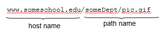
htmlfile (“a markup language”) works with browsers, including how the images/videos/scripts works -
as well as how path names work
HTTP Overview
Because we need the browser to render the page correctly, so we need reliable data transfer. Hence, HTTP protocols chooses to use TCP, with port 80
Recall: how we implemented the TCP for sockets:
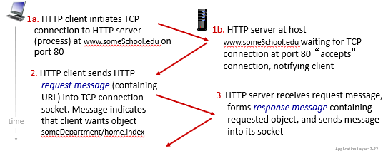
- client initiates TCP connection (creates socket) to server, port 80
- server accepts TCP connection from client
- HTTP messages (application-layer protocol messages) exchanged between browser (HTTP client) and Web server (HTTP server)
- TCP connection closed
Additionally, by DEFAULT, the protocol of HTTP is “stateless”
- yet we MADE IT stateful by using other tools such as Cookies
Disadvantage of Stateful Connections
- past history (state) must be maintained
- if server/client crashes, their views of “state” may be inconsistent, must be reconciled
- security issues!
HTTP Connections
In generally we had two types:
- Non-persistent HTTP: sending only ONE object (e.g. an image) over one connection
- then if your html has 3 images, 3
css, 1 html, then it needs 7 connections - connection terminates over each single message exchanges
- then if your html has 3 images, 3
- Persistent HTTP: multiple objects can be sent over a single TCP connection
- less overhead, better performances
- connection terminates after multiple exchanges
Non-persistent HTTP: example
Consider the case when you entered www.someSchool.edu/someDepartment/home.index
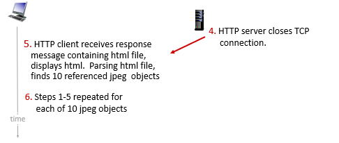
So basically this is very wasteful.
RTT (definition)
- time for a small packet to travel from client to server and back
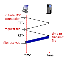
Persistent HTTP
In this case:
- server leaves connection open after sending response
- the connection to the host, has nothing to do with your path such as
/index.html(remember it is just asocket)
- the connection to the host, has nothing to do with your path such as
- subsequent HTTP messages between same client/server sent over open connection
- here we have the request, i.e.
GET /index.html blablabla
- here we have the request, i.e.
- client sends requests as soon as it encounters a referenced object
- as little as one RTT for all the referenced objects (cutting response time in half)
- the initial connection for (e.g.)
index.htmlwill still take 2 RTT, but for all other (e.g.) 10 objects on thatindex.htmlpage, we just need $10 \times 1$ RTT.
- the initial connection for (e.g.)
HTTP Message Format
HTTP Request Message
We have two types: request and response.
Each request message looks like
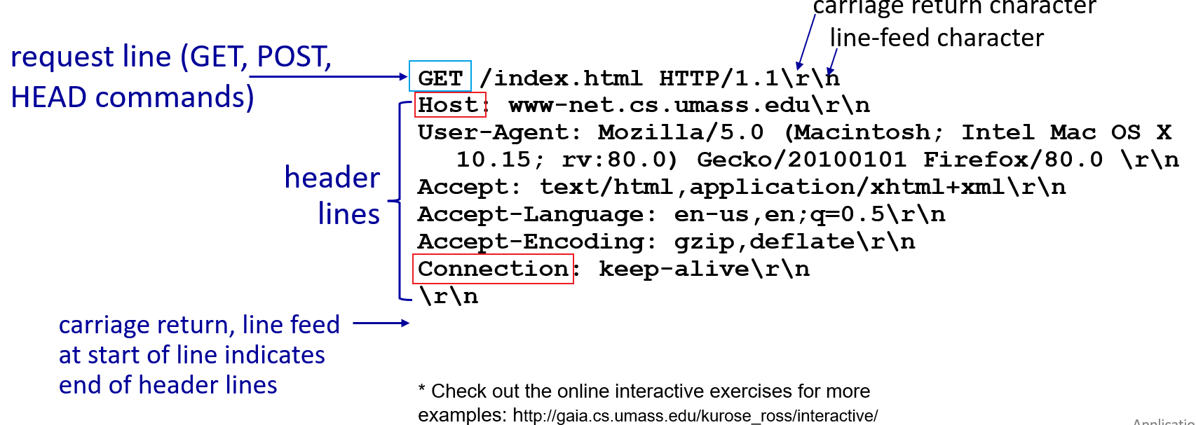
notice that:
- the connection goes to the
HOSTfield - in the connection, the
pathis queried - content is in ASCII
Moreover, remember that we can have user parameters specified with login?a=b&c=d etc.
- fundamentally this is agreed upon in the application side how to parse the stuff after
?
Conditional GET
Goal: don’t send object if cache has up-to-date cached version
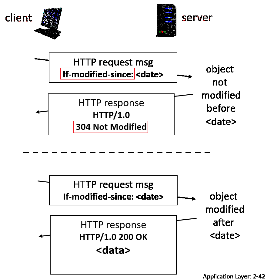
where if you get 304, then no data is actually sent over.
HTTP Response Message
An response message looks like:
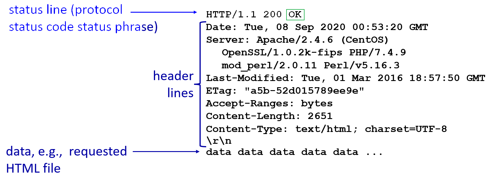
where:
- notice the
Last-Modifiedfield. This is used later by the client browser, so that the next time it requests the same resource, it will send a “send if modified” version of a get request, with this date attached. - notice that
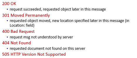
200 OKstatus code
Additionally, some other status codes:
Maintaining State: Cookies
Recall that HTTP protocol is stateless, which means each request is independent of each other.
Then, to emulate a STATEFUL request, we use cookies.
Usually, we have four components interacting when using/managing cookies:
- cookie received from header line of HTTP response message
- cookie sent (from user’s browser) header line in next HTTP request message
- cookie file kept on user’s host, managed by user’s browser
- back-end database at Web site (used for managing what to do with those cookies)
For Example
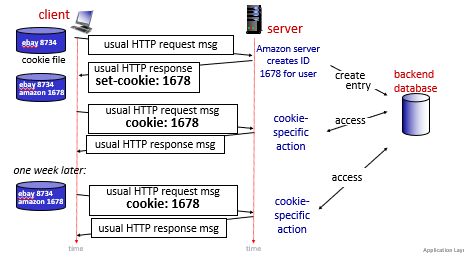
where:
- the server creates cookies and
- subsequent HTTP requests to this site will contain the cookie ID value
- the above is an example of a persistent cookie
Note
- we have session specific cookies, and persistent cookies
- session specific cookies are erased after you close your session (e.g. browser window)
- persistent cookies has an expiration date, which expires after that but stays there after you close your session
- third party persistent cookies (tracking cookies) allow common identity (cookie value) to be tracked across multiple web sites
- These are usually used for online-advertising purposes and placed on a website through a script or tag. A third-party cookie is accessible on any website that loads the third-party server’s code.
- e.g. once you shopped on Amazon for (e.g.) a pair of brown shoes, it might create some third party cookie. Then future other websites might look at that and provide you relevant ads.
HTTP/2
Goal: Solve the head of the line issue:
- what if the first request is a huge file, and subsequent are small files? The first will block the other requests.
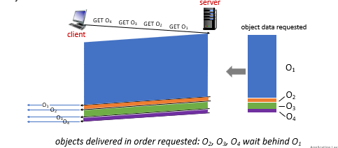
HTTP 1.1: introduced multiple, pipelined GETs over single TCP connection
- server responds in-order (FCFS: first-come-first-served scheduling) to
GETrequests in a pipe- e.g. if you requested for 10 images, they are responded/served in a FIFO
- therefore, may developers tend to still open multiple parallel connections to resolve this
However, the problem with that is:
-
with FCFS, small object may have to wait for transmission (head-of-line (HOL) blocking) behind large object(s)
-
loss recovery (retransmitting lost TCP segments) stalls object transmission
Aim of HTTP/2
One of the primary goals of HTTP/2 is to get rid of (or at least reduce the number of) parallel TCP connections for transporting a single Web page (as a resolution to Head-Of-Line blocking problem)
- TCP congestion control can also operate as intended
The HTTP/2 solution for HOL blocking is to break each message into small frames, and interleave the request and response messages on the same TCP connection.
- of course we need to then reassemble them on the other end. So this protocol has to be made clear on that.
Of course besides that, HTTP/2 also has the following features:
- Response Message Prioritization:
- the client can give a weight to each request for its priority. Numbers range from $1\to 256$. Then the server cans send first the frames for the responses with the highest priority.
- You can also states each message’s dependency on other messages by specifying the ID of the message on which it depends.
- Server Pushing: a server to send multiple responses for a single client request.
- for a single page, there is usually a lot of objects (e.g. images). Instead of waiting for the HTTP requests for these objects, the server can analyze the HTML page, identify the objects that are needed, and send them to the client before receiving explicit requests for these objects.
For Example:
In HTTP 1.1, this is the order of data sent:
For HTTP 2:
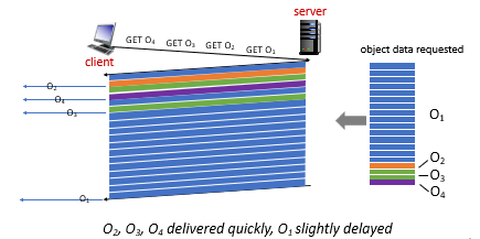
where basically you do a Round-Robin.
HTTP/3
Thought HTTP/2 is the most common now, it still has some problems. HTTP/2 over single TCP connection means:
- recovery from packet loss still stalls all object transmissions
- no security over vanilla TCP connection
HTTP/3 is yet a new HTTP protocol that is designed to operate over QUIC. As of 2020, HTTP/3 is described in Internet drafts and has not yet been fully standardized.
- QUIC (Quick UDP Internet Connections, pronounced quick) is an experimental transport layer network protocol designed by Google
- Think of QUIC as being similar to TCP+TLS+HTTP/2 implemented on UDP
HTTP/3
HTTP/3: adds security, per object error- and congestion-control (more pipelining) over QUIC (which is UDP)
- QUIC was chosen because many of the HTTP/2 features (such as message interleaving) are subsumed by QUIC
- since it is on UDP, it would be faster as well
More on HTTP/3 in transport layer chapter.
Web Caching
There are two caches:
- the caching of website made by your application
- the caching of website in a Web Cache/proxy server. Here we talk about this one.
Web Caching Server
A Web cache—also called a proxy server—is a network entity that satisfies HTTP requests on the behalf of an origin Web server.
- therefore, the Web cache has its own disk storage and keeps copies of recently requested objects in this storage
The basic diagram looks as follows, and the flow is simple:
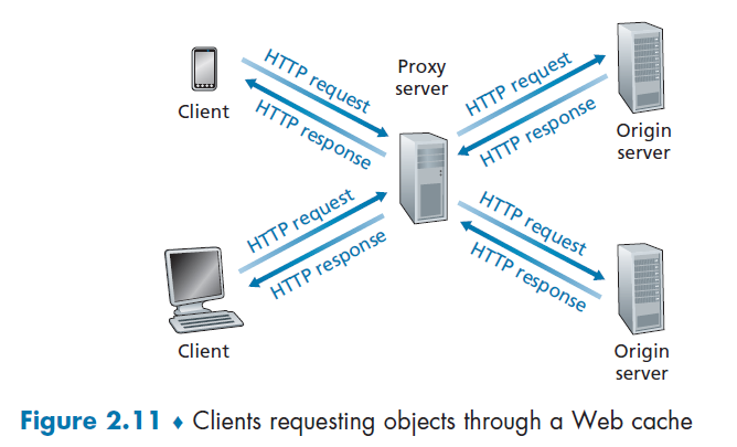
Suppose you want to get www.someschool.edu/campus.gif. (You need to configure your web browser so that all of the user’s HTTP requests are first directed to the Web cache first).
Then:
- The browser establishes a TCP connection to the Web cache and sends an HTTP request for the object to the Web cache.
- The Web cache checks to see if it has a copy of the object stored locally.
- If it does, the Web cache returns the object within an HTTP response message to the client browser.
- If the Web cache does not have the object, the Web cache opens a TCP connection to the origin server, that is, to www.someschool.edu. then sends an HTTP request
- When the Web cache receives the object, it stores a copy in its local storage and sends a copy to the client (over the existing TCP connection between the client browser and the Web cache).
So basically a cache is both a server and a client at the same time.
In reality:
- Typically a Web cache is purchased and installed by an ISP. For example, a university might install a cache on its campus network and configure all of the campus browsers to point to the cache
DNS: Domain Name System
The idea is that:
- an internet host is identified by an IP address
- an IP address assigned per network interface. So a device could have multiple IP addresses
- but we use readable formats such as
cs.umass.edu, we need to map them to IP addresses
Domain Name System
- distributed database implemented in hierarchy of many name servers
- distributed database = each database contains partial information; synchronization issue is saved
- application-layer protocol: hosts, DNS servers communicate to resolve names (address/name translation)
Disadvantage of Centralized DNS
- single point of failure
- traffic volume
- distant centralized database
- maintenance
DNS Services
Some services provided by the DNS server is:
- hostname-to-IP-address translation
- host aliasing
- Basically you can have two or more domain names that take you to a single site.
- e.g. a hostname such as
relay1.west-coast.enterprise.comcould have, say, two aliases such as www.enterprise1.com and www.enterprise.com. In this case, the hostnamerelay1.west-coast.enterprise.comis said to be a canonical hostname
- mail server aliasing
- all organization has a dedicated mail server
- e.g. Bob has an account with Yahoo Mail, which might be as simple as bob@yahoo.com. However, the hostname of the Yahoo mail server is more complicated and much less mnemonic than simply
yahoo.com. So internally there is some aliasing done.
- load distribution
- there are some replicated Web Servers: many IP addresses correspond to one name
- load balancing: depending on where the request comes from, the service can respond different IP addresses so we can load balance
For Example: Using nslookup
➜ nslookup
> www.columbia.edu
Server:         172.18.48.1
Address:        172.18.48.1#53

Non-authoritative answer:
www.columbia.edu        canonical name = www.a.columbia.edu.
www.a.columbia.edu      canonical name = www.wwwr53.cc.columbia.edu.
Name:   www.wwwr53.cc.columbia.edu
Address: 128.59.105.24
In general, DNS are used:
- trillions of queries/day
- so performance matters!
- databases contains billion records
- decentralized databases
- millions of different organizations responsible for their records
Overview of How DNS Works
where:
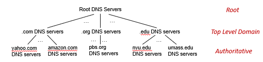
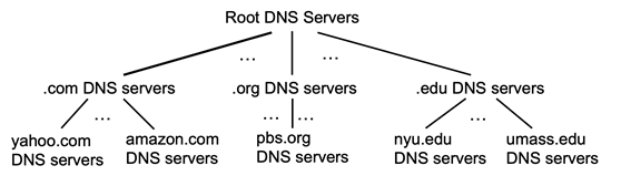
-
the root server stores IPs for the Top Level Domain servers (TLD)
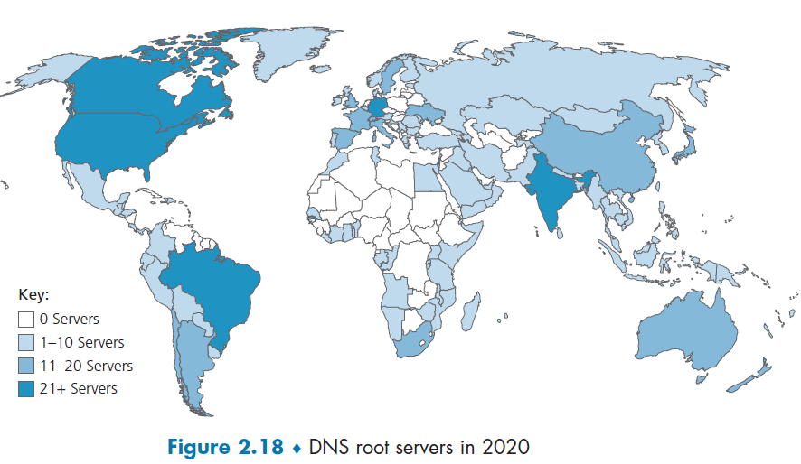
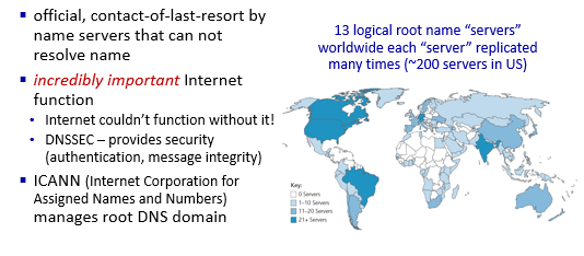
- There are more than 1000 root servers instances scattered all over the world, as shown in Figure 2.18. These root servers are copies of 13 different root servers, managed by 12 different organizations.
-
the top level domain servers knows about lower level/authoritative DNS servers
- For each of the top-level domains—top-level domains such as com, org, net, edu, and gov, and all of the country top-level domains such as uk, fr, ca, and jp—there is TLD server (or server cluster).
-
the authoritative DNS server basically keeps the actual mapping (so it is managed by the actual organization such as Amazon)
- Every organization with publicly accessible hosts (such as Web servers and mail servers) on the Internet must provide publicly accessible DNS records that map the names of those hosts to IP addresses
-
basically each parent node knows IP address of their child node
Advantages
- the benefit is that if some IP-DNS needs to be changed, only one node needs to be updated.
For Example
Client wants IP address for www.amazon.com; 1st approximation:
- client queries local DNS server first (covered in Local Name Server)
- client queries root server to find
.comDNS server - client queries
.comDNS server to getamazon.comDNS server - client queries
amazon.comDNS server to get IP address for www.amazon.com
However, in reality:
- once a name gets resolved, it will get cached locally (e.g. in your organization DNS server). This means that queries to the root DNS server is actually not a lot
- each cached name will have an expiration time. Before that name expires, you cannot load balance using CDN obviously.
Root Name Server
Top Level Domain Server
Knows about authoritative DNS servers, who stores the actual mapping you need.
Authoritative DNS servers:
- organization’s own DNS server(s), providing authoritative hostname to IP mappings for organization’s named hosts can be maintained by organization or service provider
Local Name Server
This is where things get cached and can be reducing the number of requests to the root server.
So technically, when host makes DNS query, it is first sent to its *local* DNS server
- Local DNS server returns reply if it has been cached
- Forwarding request into DNS hierarchy for resolution if it doesn’t know
local DNS server doesn’t strictly belong to hierarchy
ipconfigWhen you type that command in Windows, you get something like:
DNS 服务器  . . . . . . . . . . . : 128.59.1.3
                                   128.59.1.4
and those would be your local name server address
- those are configured once you connect to the WiFi/network
Iterative Query
Now we talk about how DNS actually works.
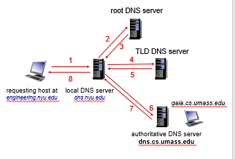
the advantage of this is:
- your local server can cache also Top Level DNS Server IP, Authoritative DNS Server IP
Recursive Query
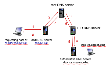
this is rarely used due to its problem of
- heavy load on root DNS server
- caching less stuff
In reality, it is more often to see a combination of iterative and recursive approaches.
DNS Records and Messages
DNS distributed database store resource records (RRs), which contains mappings from Domain to IP.
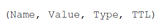
Resource Record
A single record is a four tuple
where:
TTL is the time to live of the resource record; it determines when a resource should be removed from a cache.
- we ignore this field for examples below
Types assign meanings to Name and Value
Type Name Value Example A Hostname IP Address (relay1.bar.foo.com, 145.37.93.126, A)NS Domain Hostname of an authoritative DNS server that knows the IP of this domain (used for build DNS route) (foo.com, dns.foo.com, NS)CNAME alias hostname canonical hostname (foo.com, relay1.bar.foo.com, CNAME)MX alias hostname canonical name of a mail server (foo.com, mail.bar.foo.com, MX)
DNS Messages
Therefore, each DNS reply message carries one or more resource records.
In general, we have two types:
- DNS query messages
- DNS reply messages
But both query and reply messages have the same format
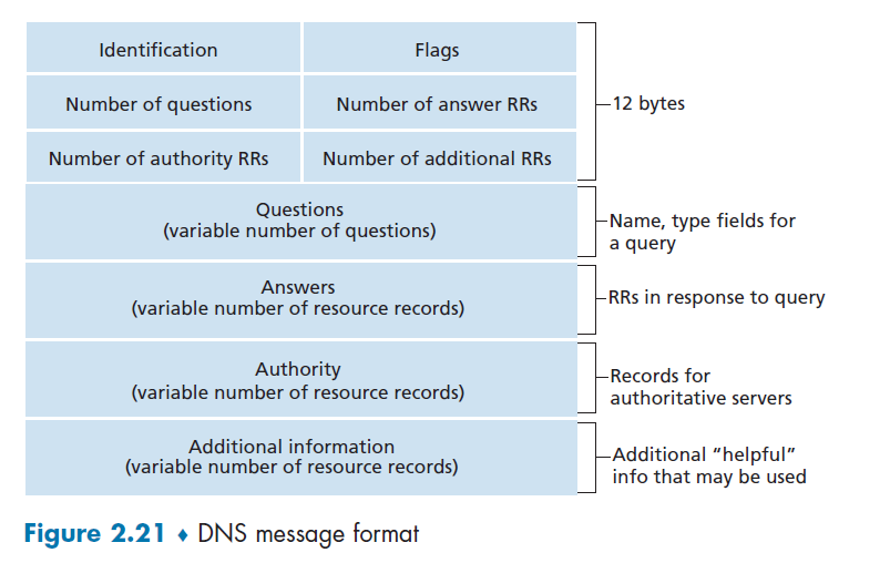
where:
- Identification: 16-bit number that identifies the query. This identifier is copied into the reply message to a query, allowing the client to match received replies with sent queries.
- Flags: Basically a bitmap, with each bit:
- 1-bit query/reply flag indicates whether the message is a query (0) or a reply (1).
- 1-bit authoritative flag is set in a reply message when a DNS server is an authoritative server for a queried name.
- 1-bit recursion-desired flag is set when a client (host or DNS server) desires that the DNS server perform recursion
- 1-bit recursion-available field is set in a reply if the DNS server supports recursion.
- Number of xxx: number of occurrences of the four types of data sections that follow the header
- Questions: this section contains information about the query that is being made. This section includes
- a name field that contains the name that is being queried
- type field that indicates the type of question (e.g. type
MX)
- Answer : contains the resource records (i.e. four tuples) for the name that was originally queried
- The rest is labelled
Inserting Records into DNS Database
Suppose you have just created an exciting new startup company called Network Utopia. Then you might want to have your own authoritative DNS running so you can deliver content.
-
register the domain name networkutopia.com at a registrar (i.e. buy it from somewhere)
- A registrar is a commercial entity that verifies the uniqueness of the domain name, enters the domain name into its DNS database (as discussed below), and collects a small fee from you for its services.
-
provide the registrar with the names and IP addresses of your primary and secondary authoritative DNS servers
-
e.g.
dns1.networkutopia.com,dns2.networkutopia.com,212.2.212.1, and212.212.212.2. -
then the registrar would then make sure that a Type NS and a Type A record are entered into the TLD com server
(networkutopia.com, dns1.networkutopia.com, NS)
(dns1.networkutopia.com, 212.212.212.1, A)
-
-
Then, in your authoritative DNS server:
- Type A resource record for your Web server www.networkutopia.com and the Type MX resource record for your mail server
mail.networkutopia.comare entered into your authoritative DNS servers.
- Type A resource record for your Web server www.networkutopia.com and the Type MX resource record for your mail server
-
Once all of these steps are completed, people will be able to visit your Web site at www.networkutopia.com and send e-mail to the employees at your company
Then, one someone wanted to visit, the following would actually happen:
- host will first send a DNS query to her local DNS server.
- The local DNS server will then contact a TLD com server. (The local DNS server will also have to contact a root DNS server if the address of a TLD com server is not cached.)
- The TLD com server sends a reply to Alice’s local DNS server, with the reply containing the two resource records of TYPE A and TYPE NS.
- The local DNS server then sends a DNS query to
212.212.212.1, asking for the Type A record corresponding to www.networkutopia.com - Then your authoritative DNS server needs to respond, say
212.212.71.4, which is the IP of your webserver - Alice’s browser can now initiate a TCP connection to the host 212.212.71.4 and send an HTTP request over the connection
DNS Security
In reality, there were two types of attacks on DNS servers.
- DDoS attacks
- bombard root servers with traffic
- not successful to date, since we can do traffic filtering
- bombard TLD servers
- bombard root servers with traffic
- Spoofing attacks
- intercept DNS queries, returning bogus replies
- DNS cache poisoning
Facebook DNS Outrage
Recall that in the end, we will get an IP address. But we still needs to get to that IP address physically.
- each router needs to tell other routers which destination it can reach, by some announcement.
Facebook DNS Outrage
- Some configuration were mistaken, so Facebook routers starts to withdrawn their connection to every ISP. As a result, physically no routing exists to reach a Facebook DNS Server
- Then, due to the absence of DNS requests, those DNS server thought there is an error so they shutted down
- In the end, now there is both NO ROUTES and NO ALIVE DNS. So nobody can actually reach Facebook’s servers.
Video Streaming and Content Distribution Networks
By many estimates, streaming video—including Netflix, YouTube and Amazon Prime—account for about 80% of Internet traffic in 2020. Things to take into account:
- heterogeneity of uses (e.g. bandwidth available)
- need to scale to 1 billion + users
This section discusses how popular video streaming services are implemented in today’s Internet.
- a distributed, application-level infrastructure
Internet Video.
Basically, for pre-recorded videos
- servers have a copy of them
- users send requests to the servers to view the videos on demand
Bit Rate
Bit rate is the number of bits that are conveyed or processed per unit of time.,
- each video is a sequence of images with certain FPS (frame per second)
- each frame/image has a number of pixels
- each pixel is represented by some bits
Then some algorithm can compress those bits per second by utilizing redundancy within and between images (a like
zipcompression techniques). So we need less bits per image = less bits rate.
- spatial compression + temporal compression
But obviously, the higher the bit rate, the better the quality = the higher the bandwidth requirement.
In reality, we then have:
- CBR (constant bit rate), such that video encoding rate is fized
- VBR (variable bit rate), video encoding rate changes depending on amount of spatial and temporal compression we have
- i.e. when a scene changes to a new one, compression changes.
- so to preserve high quality, this is the way
HTTP Streaming and DASH
Now, we know how video is “played”. Here we talked about how to store and deliver the video such that it can be played as mentioned before.
Consider for the simple case
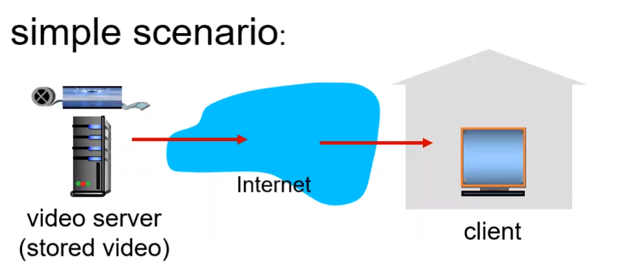
the main problem we are facing is therefore:
- clients tend to have variable bandwidth
- clients might have various packet loss, delay, congestion
Then, in this model, we have:
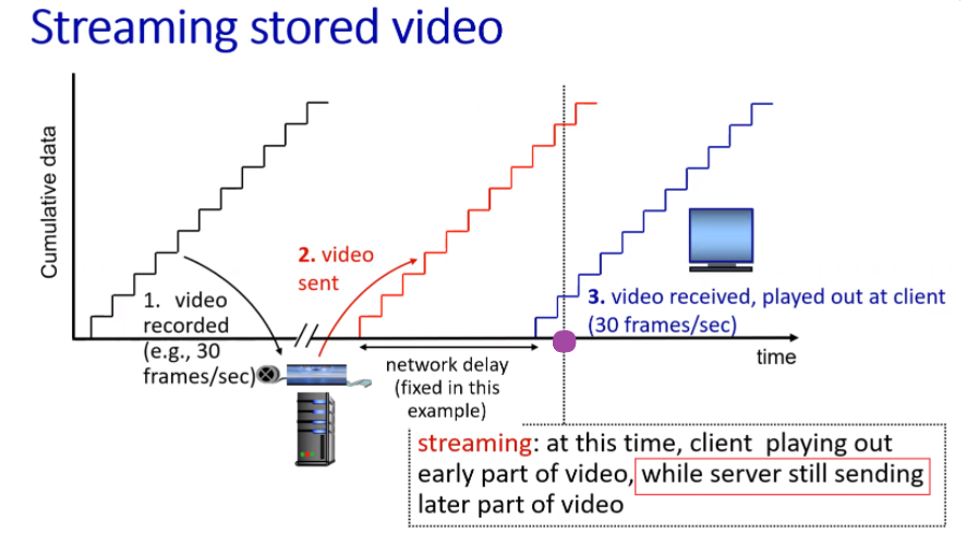
where:
- we assumed some CBR
- due to some network delay, video plays at line 3
- at the time of play, we stored (about) 1 second of received video. So essentially we are still receiving data while playing.
Playback
Once the number of bytes (for the video) in client’s buffer buffer exceeds a predetermined threshold, the client application begins playback — specifically, starts playing by grabbing images from the buffer.
What happens yet in reality is:
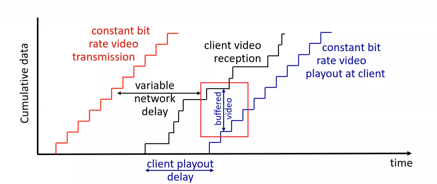
where:
- due to the variable network condition, we might need to buffer quite some so that client won’t need to “re-buffer”/pause in the video
- if the black curve intersects with blue curve, we need “re-buffering/pausing” on client side = bad experience
Need Variable Bit Rate
Therefore, when client detects that the two curves are about to intersect, it will lower the bit rate of requested video, so that it can buffer = make sure smooth client experience.
- client experience include fast forward, rewind, etc.
To realize this, this is done by DASH.
Problem with HTTP:
- All clients receive the same encoding of the video, despite the large variations in the amount of bandwidth available to a client, both across different clients and also over time for the same client
DASH - Dynamic Adaptative Streaming over HTTP
In DASH, the video is
- divided in to multiple chunks
- each chunk is encoded into several different versions, with each version having a different bit rate
Therefore, the idea is that:
Server
- holds all those different chunks + versions
- holds a
manifestfile, with a mapping ofurlfor each different chunk - all those chunks=files are then replicated in CDN nodes
Client
- request the
manifestfile- note that this file is the same for all users for the same resource
- periodically estimate the bandwidth
- decide to request for which chunk of video depending on observer bandwidth, and consults the
manifestfor actual request- so we can have different bit rates over time if needed
- so all the intelligence is at client, decides when to request, what bit rate to request, and where to request (
manifest+ closest CDN node)
- use the
urlon themanifestand get the chunk from a CDN node- recall that DNS server is the one that decides which CDN node your data will be from, by look at the
source ip.
- recall that DNS server is the one that decides which CDN node your data will be from, by look at the
Note: when actually sending each chunk, it is done by HTTP
GETrequest messages.
CDN - Content Distribution Networks
Now, the idea is that we prefer having receiving file from geographically close sites.
CDNs typically adopt one of two different server placement philosophies:
- Enter Deep. One philosophy, pioneered by Akamai, is to enter deep into the access networks of Internet Service Providers, by deploying server clusters in access ISPs all over the world
- so we get really close to end users, which means there are clusters in thousands of locations
- smaller storage size
- Bring Home. A second design philosophy, taken by Limelight and many other CDN companies, is to bring the ISPs home by building large clusters at a smaller number (10s)
- lower maintenance and management overhead, but a bit larger delay
- larger storage size
Then, once its clusters are physically in place, the CDN replicates content across its clusters.
Pulling Contents
- The CDN may not want to place a copy of every video in each cluster, since some videos are rarely viewed or are only popular in some countries. In fact, many CDNs do not push videos to their clusters but instead use a simple pull strategy: if request file is not stored in the CDN node, it will retrieve it and store the copy.
- When cluster’s storage is full, it removes the least frequently requested video
Note:
- Above are third-party CDNs, which distribute contents for other content providers.
- There is also private CDN, that is, owned by the content provider itself; for example, Google’s CDN distributes YouTube videos and other types of content.
Load Balancing with DNS
The trick to load balance between CDN nodes is that:
- each
urltoiptranslation is essentially done by a DNS server. So we can store a shortexpirationtime such that it will frequently go to the authoritative DNS server- then authoritative DNS server can then tell you which CDN cluster to use for load balancing purposes.
- then even inside the CDN cluster, you could have some load balancing for which CDN node to use
CDN Operation
Here we demonstrate how DNS + CDN cluster works.
Suppose that you wanted to watch the film Transformers 7, which on NetCinema.com has the url of http://video.netcinema.com/6Y7B23V. Then, the following would happen:
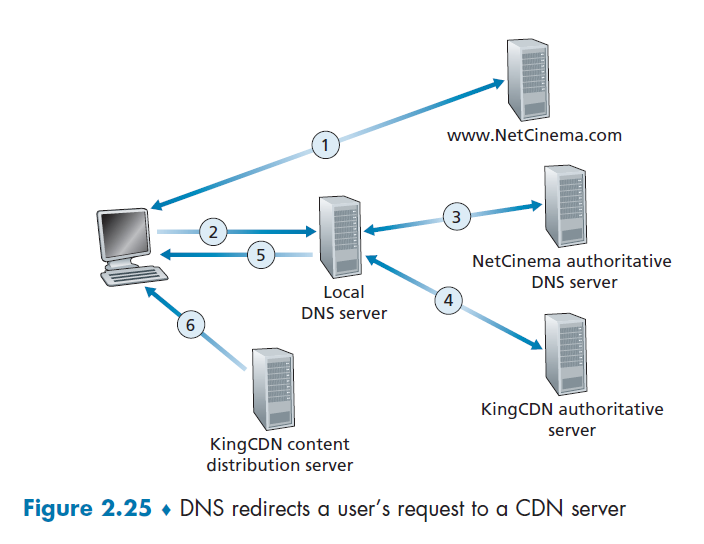
- The user visited the Web page at
netcinema.comand got http://video.netcinema.com/6Y7B23V - The user clicked http://video.netcinema.com/6Y7B23V to watch the film, which then sends a DNS query for
video.netcinema.com - First it goes to the Local DNS server (LDNS), which then handles the query to the authoritative DNS of NetCinema
- now, instead of returning an IP address, the NetCinema authoritative DNS server returns to the LDNS a hostname in the KingCDN’s domain:
a1105.kingcdn.com
- now, instead of returning an IP address, the NetCinema authoritative DNS server returns to the LDNS a hostname in the KingCDN’s domain:
- Then, the DNS query enters into KingCDN’s private DNS infrastructure. Now, for
a1105.kingcdn.com.- here, it can decide which CDN node to use.
- KingCDN’s DNS system eventually returns the IP addresses of a KingCDN content server node to the LDNS, and LDNS forwards the IP address of the content-serving CDN node to the user’s host
- The users received an
ipfrom the KingCDN node, and will establish the TCP connection there and request for the data.- here, if DASH is used, the server will first respond with a
manifestand etc.
- here, if DASH is used, the server will first respond with a
Peer-to-Peer File Distribution
The applications described in this chapter thus far—including the Web, e-mail, and DNS—all employ client-server architectures with significant reliance on always-on infrastructure servers.
There is minimal (or no) reliance on always-on infrastructure servers. Instead, pairs of intermittently connected hosts, called peers, communicate directly with each other.
- e.g. file distribution (BitTorrent): each torrent address will be a “directory” to the specific peer-to-peer network
- you can download any part of the file first (e.g. the last part might comes first)
- e.g. Streaming (KanKan): we need to download from the first part
- e.g. VoIP (Skype, originally)
Basically the advantage is that your P2P will be self-scaling since each host is also an uploader/server
Scalability of P2P Architecture
We want to compare the ideal performance of client-server and p2p.
Consider the case when we need to deliver a large file to a larger number of hosts. You will see that:
- In client-server file distribution, the server must send a copy of the file to each of the peers
- In p2p, each peer can redistribute any portion of the file it has received to any other peers.
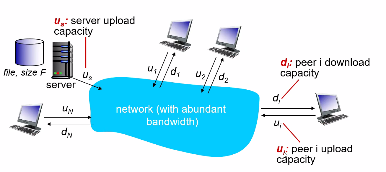
Let there be $F$ bits of a file to be send, and there are $N$ users. Let the upload speed be $u$, and download speed be $d$. We want to compare the distribution time - the time it takes to get a copy of the file to all N peers:
- (assumption that the Internet core has abundant bandwidth, implying that all of the bottlenecks are in access networks)
Then, we can compute that
-
Distribution time for client-server model $D_{cs}$:
The idea is that we either have server uploading the file into the client or client downloading from server.
-
The server must transmit one copy of the file to each of the $N$ peers. Thus, the server must transmit $NF$ bits. Since the server’s upload rate is $u_s$, the time to distribute the file must be at least $NF/u_s$.
-
the slowest client will have $d_{min}=\min{d_1,…,d_N}$. So if everyone downloads, we have $F/d_{min}$
so distribution time is:
-
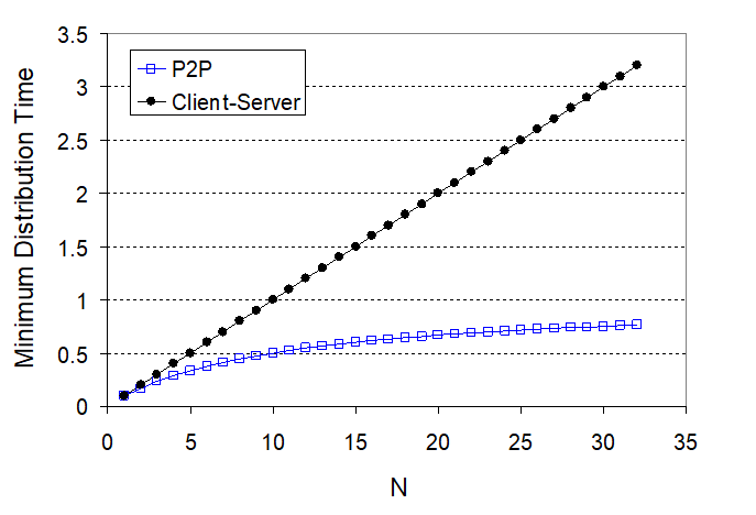
notice that $NF/u_s$ increases with $N$ linearly
-
Distribution time for P2P.
The main difference is that when a peer receives some file data, it can use its own upload capacity to redistribute the data to other peers. Therefore:
- If only server has the file, and we assume that each client starts redistributing immediately when they get a bit, then the minimum distribution time is at least $F/u_s$
- The worst case for downloading is that all bits goes to the same host with $d_{min}$. Then in that case, we have $F/d_{min}$.
- The last case is when each host has some share of the file, then to make sure everyone has all $F$ bits, we need to have uploaded $NF$ bits (to each other) with no faster than $u_{\text{total}} =u_s + \sum u_i$. Therefore, in this case, the distribution time is $NF/(u_s + \sum u_i)$.
so performance is:
\[D_{P2P} \ge \max \left\{ \frac{F}{u_s}, \frac{F}{d_{min}},\frac{NF}{u_s + \sum u_i}\right\}\]
notice that the term $NF/(u_s + \sum u_i)$ means increasing $N$ increases both $NF$ and $\sum u_i$. So eventually, this term flattens out even when $N$ is large.
P2P File Distribution
In reality, we would first divide the file into 256Kb chunk, and each host will own some of the chunks.
- $NF/(u_s + \sum u_i)$ in the P2P means we want the peer to become a server as soon as possible
- if you waited for the entire file to be a server, that will take quite a long time/wasted
Tracker
- Each torrent has an infrastructure node called a tracker. When a peer joins a torrent, it registers itself with the tracker and periodically informs the tracker that it is still in the torrent.
- Therefore, the tracker keeps track of the peers that are participating in the torrent.
Then, how P2P works is:
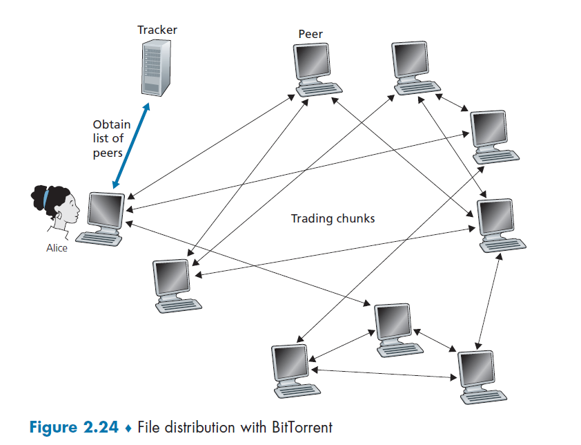
where basically when Alice clicked the magnet link:
-
obtains a list of peers from tracker, and ask the peers for a list of chunks of the file they have
- basically gives you the IP of the peers, then each peer gives you a list of what they have
- let there be $L$ neighbors. Then you get $L$ lists of chunks
-
register yourself to tracker
-
requests missing chunks from peers, rarest first. (the chunks that are the rarest/fewest copies among her neighbors)
-
compute from the $L$ list of chunks which one is the rarest
-
the rarest first is the key, with the aim of maintaining high availability
-
-
while gathering chunks, Alice also sends chunks to some of other peers (algorithm deciding who to send: Tit-for-Tat)
- unchoked peers - send to four peers who are sending Alice the data at the highest rate (reevaluate top 4 every 10 secs)
- optimistically unchoked - in addition, randomly select a new peer and send chunks every 30 seconds (this randomly selected peer MAY become the top 4 later - optimistic)
- chocked - all peers beside the above 5 are not sent data to.
The upshot is that, the in total 5 peers you are sending to would be:
- peers capable of uploading at compatible rates tend to find each other
- random neighbor selection also allows new peers to get chunks, so that they can have something to trade
-
When Alice is done, she will leave and no longer in the network anymore
Chapter 3 Transport Layer
Principles behind transport layer services:
- multiplexing, demultiplexing
- reliable data transfer
- flow control
- congestion control
Technically, reliability/flow control/congestion can also be implemented at other layers (e.g. Application, WIFI itself might cater to that by implementing in app layer), so the concept is more important in this case.
- so the idea is that those concepts goes beyond the transport layer
Commonly, there are two protocols:
- TCP, UDP
Transport Services and Protocol
A transport-layer protocol provide logical communication channel (a socket) between application
- the physical one could include many links in a path
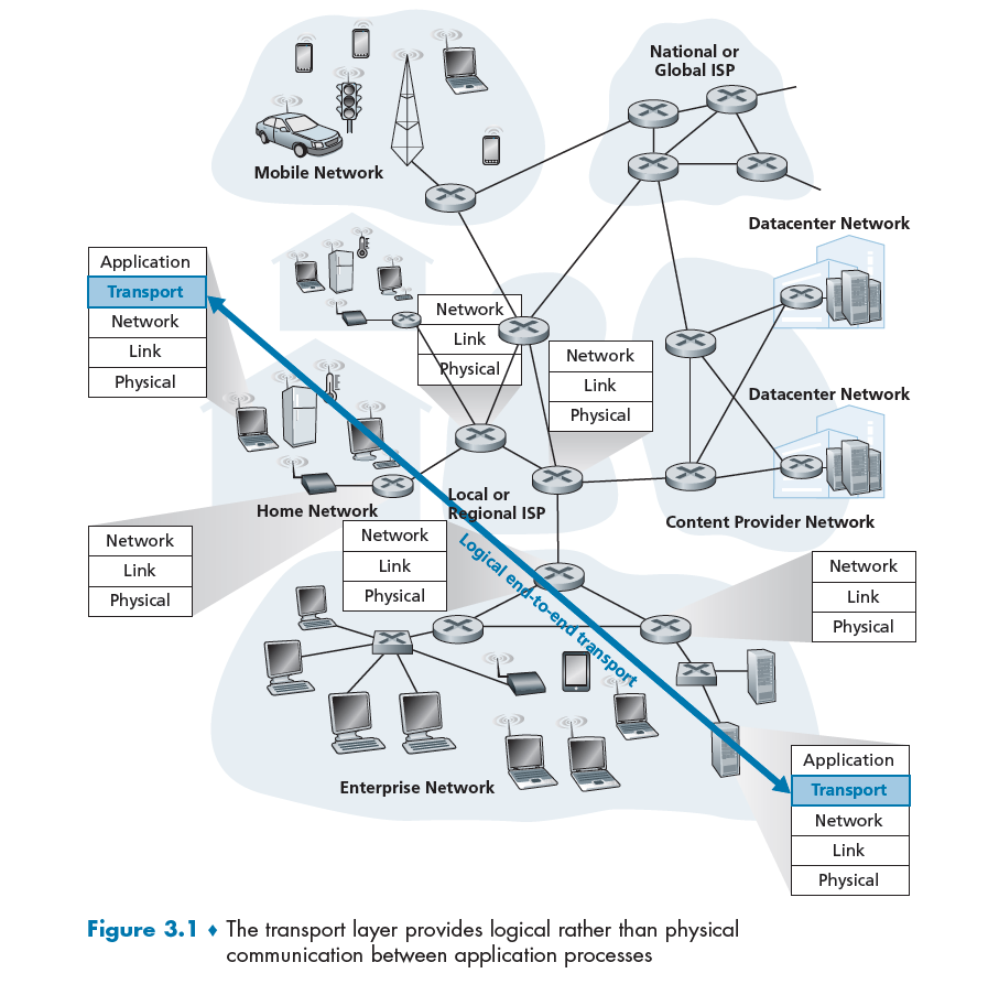
where notice that:
- transport-layer protocols are implemented in the end systems but not in network routers. Makes sense since their job is to cater to application.
Sender in Network Layer
- breaks application messages into segments (i.e. packets), add transport-layer headers, and passes to network layer
- the network later will then have the segment encapsulated within a network-layer packet (a datagram) and sent to the destination
- in the end network routers act only on the network-layer fields of the datagram
Receiver in Network Layer
-
from below, the network layer extracts the transport-layer segment from the datagram and passes the segment up to the transport layer.
-
the transport layer then processes/reassembles the segments into messages, passes to application layer
Household Analogy
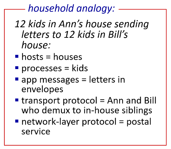
So the idea is that
- network layer: logical communication between hosts (get into the right house)
- transport layer: logical communication between processes (when in the correct house, get to the right kid)
- also note that the work of being in the house + give to the right kid means transport layer is not in the network core
Multiplexing and Demultiplexing
The idea is to extending the host-to-host delivery service provided by the network layer to a process-to-process delivery service for applications running on the hosts (which is what we need to do in transport layer)
- for this purpose, each transport-layer segment has a set of fields in the segment
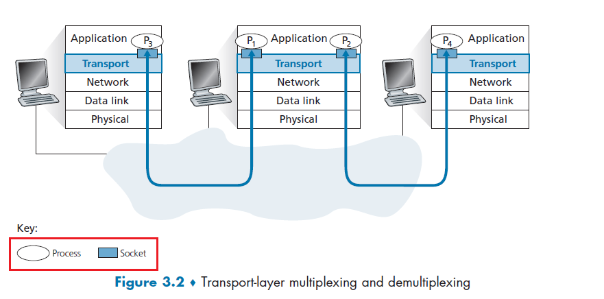
Demultiplexing
At the receiving end, the transport layer examines these fields to
- identify the receiving socket
- then directs the segment to that socket.
This job of delivering the data in a transport-layer segment to the correct socket is called demultiplexing
Multiplexing
Then obviously this does the opposite, at the sending end:
- Gathering data chunks at the source host from different sockets
- encapsulating each data chunk with header information (that will later be used in demultiplexing) to create segments
- finally passing the segments to the network layer
Note that:
- It’s important to realize that they are concerns whenever a single protocol at one layer (at the transport layer or elsewhere) is used by multiple protocols at the next higher layer
From the discussion above, we know that transport-layer multiplexing requires
- that sockets have unique identifiers
- that each segment have special fields that indicate the socket to which the segment is to be delivered
This is done by source port number and destination port number.
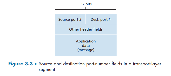
Then each socket in the host could be assigned a port number, and when a segment arrives at the host, the transport layer examines the destination port number in the segment and directs the segment to the corresponding socket.
- this is basically how UDP does it. What TCP does it is slightly different.
UDP (De)Multiplexing
Recall that we had in programming:
Host:
serverPort = 19157
# create socket
serverSocket = socket(AF_INET, SOCK_DGRAM)
serverSocket.bind(('', serverPort))
# etc
Client
serverPort = 19157
# creates socket
clientSocket = socket(AF_INET, SOCK_DGRAM) # assigns a random port for client, e.g. 46428
message = "some message"
clientSocket.sendto(message.encode(), ('localhost', serverPort)) # sends to a queue
Suppose a process in Host A, with UDP port 19157, wants to send a chunk of application data to a process with UDP port 46428 in
Host B. Then
- The transport layer in Host A creates a transport-layer segment that includes the application data, the source port number (
19157), the destination port number (46428), and two other values (discussed later)- the source port will be used by the UDP on the client to reply (in a new connection)
- transport layer then passes the resulting segment to the network layer.
- The network layer encapsulates the segment in an IP datagram and makes a best-effort attempt to deliver the segment to the receiving host
- If the segment arrives at the receiving Host B, the transport layer at the receiving host examines the destination port number in the segment (
46428) and delivers the segment to its socket identified by port46428.
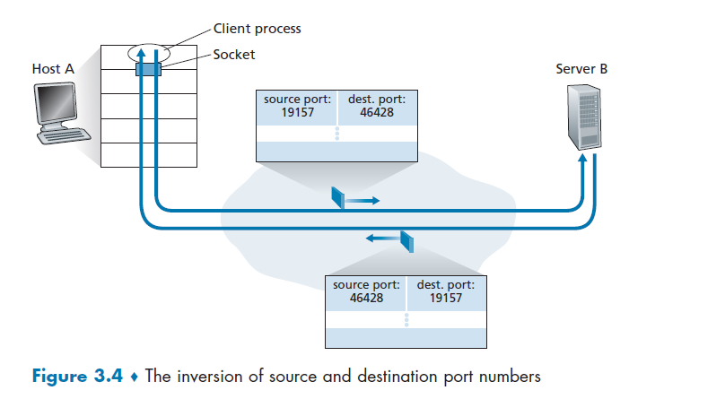
To distinguish with Socket to Send
UDP socket is fully identified by a two-tuple consisting of
\[(\text{destination IP}, \text{destination Port})\]
- because we cannot send replies directly without starting a new connection!
if two UDP segments have different source IP addresses and/or source port numbers, but have the same destination IP address and destination port number, then the two segments will be directed to the same destination process via the same destination socket
Note:
- though we only needed two tuples, all four including the IP addresses are there, it is just not used.
TCP (De)Multiplexing
Up on front, we show the difference
To distinguish with Socket to Send
TCP socket is fully identified by a four-tuple consisting of
\[(\text{source IP}, \text{source Port}, \text{destination IP}, \text{destination Port})\]
- because each client has its own persistent socket!
- the host uses all four values to direct (demultiplex)
if two TCP segments have different source IP addresses and/or source port numbers, but have the same destination IP address and destination port number, then the two segments will be directed to the DIFFERENT destination process.
- with the exception of a TCP segment carrying the original connection-establishment request (i.e. when we first called the
server_socket.accept(), multiple segments of different source goes into the same server port)
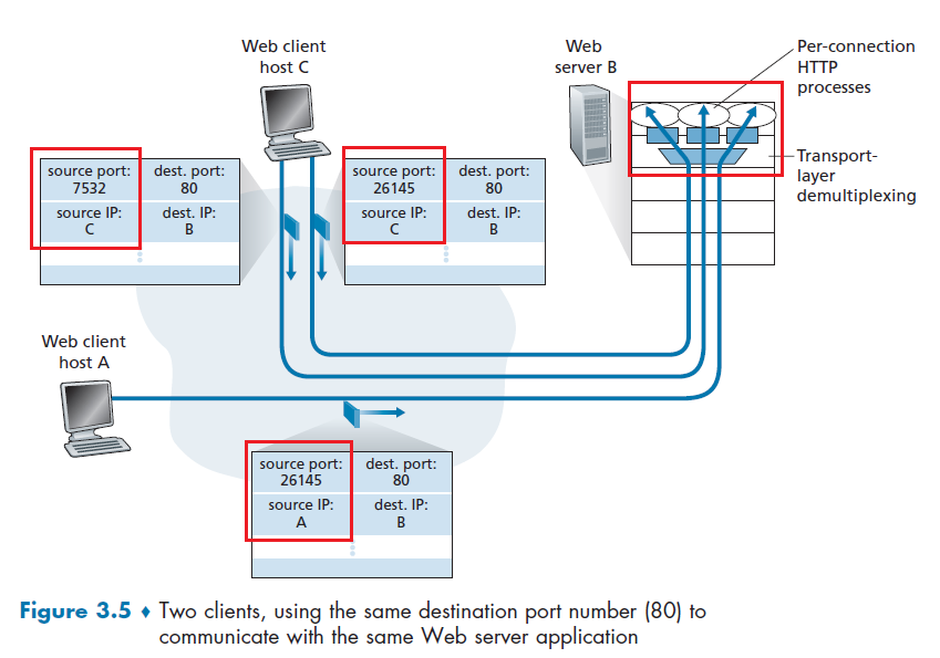
-
The TCP server application has a “welcoming socket,” that waits/listens for connection establishment requests from TCP clients (see Figure 2.29) on port number
12000 -
The TCP client creates a socket and sends a connection establishment request segment
clientSocket = socket(AF_INET, SOCK_STREAM) # some random port number assigned clientSocket.connect((serverName,12000)- A connection-establishment request is just a TCP segment with destination port number
12000+ source port number + a special connection-establishment bit set in the TCP header.
- A connection-establishment request is just a TCP segment with destination port number
-
The TCP server accept a connection on port number The server process then creates a new socket
connectionSocket, addr = serverSocket.accept() -
The transport layer at the TCP server notes the following four values in the connection-request segment:
- source port number in the (connection-request) segment
- the **IP address of the source host **in the (connection-request) segment
- the new forked destination port number (
addr) - its own IP address.
The newly created connection socket is identified by these four values.
User Datagram Protocol
A no-frills, bare-bones transport protocol. Aside from the multiplexing/demultiplexing function and some light error checking, it adds nothing to IP protocol.
UDP usages:
-
streaming multimedia apps (loss tolerant, rate sensitive)
-
DNS
-
SNMP
-
HTTP/3
if reliable transfer needed over UDP (e.g., HTTP/3):
-
add needed reliability at application layer
-
add congestion control at application layer
Short Summary
In fact, if the application developer chooses UDP instead of TCP, then the application is almost directly talking with IP.
UDP takes messages from the application process, attaches source and destination port number fields for the multiplexing/demultiplexing service, adds two other small fields, and passes the resulting segment to the network layer.
UDP Action
- is passed an application-layer message to transport layer
- transport layer uses UDP, so add a small fields of ports, length and checksum. This becomes a UDP segment now.
- network layer encapsulates the transport-layer segment into an IP datagram and then makes a best-effort attempt to deliver the segment to the receiving host
On the receiver side:
-
network layer received an IP segment, extracts the UDP segment and pass it up to transport layer
-
transport layer, with UDP, which now has a UDP segment:
- checks UDP checksum
- extract application message
-
uses the destination port number to deliver the segment’s data to the correct application process
- pass it to application layer
-
application layer receives the application message.
Advantages of UDP
- Finer application-level control over what data is sent, and when.
- As compare to TCP, which might throttle your message with its congestion control protocol.
- No connection establishment.
- As we’ll discuss later, TCP uses a three-way handshake before it starts to transfer data
- No connection state.
- since once you sent the packet, you are done. There is no connection.
- Small packet header overhead.
UDP Segment Structure
Therefore, following from the above discussion, the content looks like
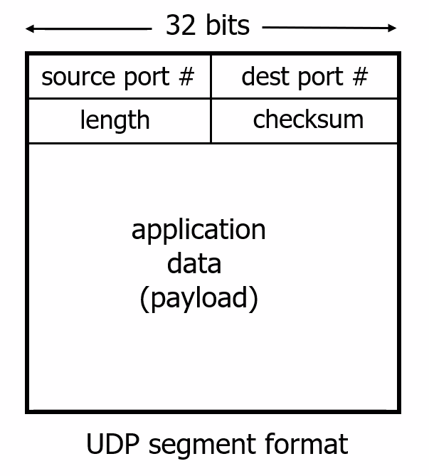
where:
- the source IP and destination IP will then be in the IP protocol packet
- the port numbers allow the destination host to pass the application data to the correct process running on the destination end system
UDP Checksum
Goal: detect errors (i.e. flipped bits) in transmitted segment, by computing 1s complement of the sum of all the 16-bit words in the segment
Basically, the sender will:
- send the data (in payload)
- send the checksum of the data
The receiver will:
- receive the data, compute the checksum from it
- compare with the received checksum
Although UDP provides error checking, it does not do anything to recover from an error.
- Some implementations of UDP simply discard the damaged segment;
- others pass the damaged segment to the application with a warning. (so that application layer can implement recovery/request for retransmission)
Disadvantage
- Since if one bit of the data is flipped, the entire packet needs to be retransmitted. This means that the application needs to then request again
->costs times and round trips.
For Example:
Data is two lines of 16 bit numbers:
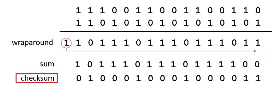
so technically there are errors that a checksum won’t detect. But the chances of that happening is low.
-
then, to check the checksum, it takes 1's complement of the sum of the data (including) checksum. If all correct, it should be all 0s.
			   10101001
               00111001
               00011101 // checksum
               --------
   Sum         11111111
   Complement  00000000  means that the pattern is O.K.
where notice that you sum the checksum as well.
UDP Summary
“no frills” protocol:
- segments may be lost, delivered out of order
- best effort service: “send and hope for the best”
UDP has its plusses:
- no setup/handshaking needed (no RTT incurred)
- can function when network service is compromised
- helps with reliability (checksum)
build additional functionality on top of UDP in application layer (e.g., HTTP/3)
Principle of Reliable Data Transfer
Problem of implementing reliable data transfer occurs not only at the transport layer, but also at the link layer and the application layer as well. So here it is an abstraction of how to ensure reliability on a high level.
The idea of having this (before introducing TCP) is
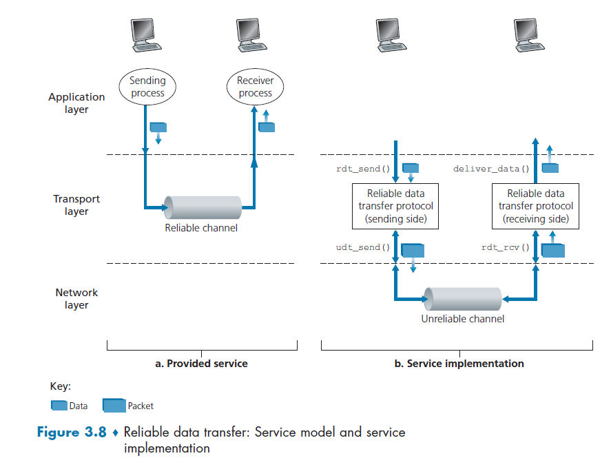
In the above figure:
- reliability happens to be implemented on Transport Layer, and any layer below the Transport Layer may be unreliable
- the sending side/application calls `rdt_send()`. It will pass the data to be delivered to the upper layer at the receiving side. (
rdtfor reliable data transfer) - On the receiving side,
rdt_rcv()will be called when a packet arrives from the receiving side of the channel. - When the
rdtprotocol wants to deliver data to the upper layer, it will do so by callingdeliver_data(), i.e. called by the `rdt` protocol implementation - so basically you need to implement whatever is between
rdt_send()andudt_send();deliver_data()andrdt_rcv()
Note
- TCP basically makes it look like being reliable above the network layer (below it is it unreliable)
- UDP does nothing, so it is hence no better than network layer unreliability
In particular, note that the possibility of being unreliable at network layer would be, in descending order of complexity:
- packet being lost (no idea if it is sent in the beginning)
- packet having corrupted data
- packet out of order
To ensure reliability through them. the idea is to exchange message about the state of each other.
Building a Reliable Data Transfer Protocol
FSM: Finite State Machine. We will use this to illustrate how to deal with each case of error mentioned above.
- The initial state of the FSM is indicated by the dashed arrow.
- The event causing the transition is shown above the horizontal line labeling the transition, and the actions taken when the event occurs are shown below the horizontal line
Simplest Case: RDT1.0
simplest case, in which the underlying channel is completely reliable.
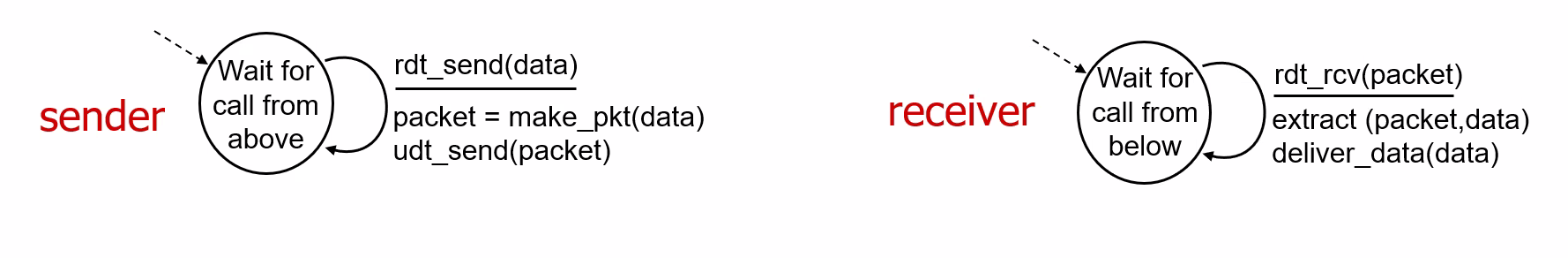
where:
- there are separate FSMs for the sender and for the receiver
Sender
- sending side of simply accepts data from the upper layer via the
rdt_send()event (e.g. application called it). Then, it does:- creates a packet containing the data
packet=make_pkt(data) - sends the packet into the channel
udt_send(packet)
- creates a packet containing the data
Receiver
rdtreceives a packet from the underlying channel via therdt_rcv(packet)event (e.g. network layer called it) then:- removes the data from the packet (via the action
extract(packet, data)) - passes the data up to the upper layer (via the action
deliver_data(data)).
- removes the data from the packet (via the action
This is simple because a perfectly reliable channel means: there is no need for the receiver side to provide any feedback to the sender since nothing can go wrong
Bit Error: RDT2.0
When there are some bit errors (e.g. checksum didn’t match)
- Such bit errors typically occur in the physical components of a network as a packet is transmitted, propagates, or is buffered.
- We’ll continue to assume for the moment that all transmitted packets are received (although their bits may be corrupted) in the order in which they were sent.
Then, to recover, you tell the sender of a Negative Acknowledgement (NACK) (i.e. not understood/received)
Acknowledgements (ACKs): receiver explicitly tells sender that pkt received OK
Negative Acknowledgements (NAKs): receiver explicitly tells sender that pkt had errors
Therefore, if sender receives a NAK, then it will retransmit the packet.
- stop of wait: sender sends one packet, then waits UNTIL received a response from the receiver
- In a computer network setting, reliable data transfer protocols based on such retransmission are known as ARQ (Automatic Repeat reQuest) protocols.
The sender side FSM looks like:
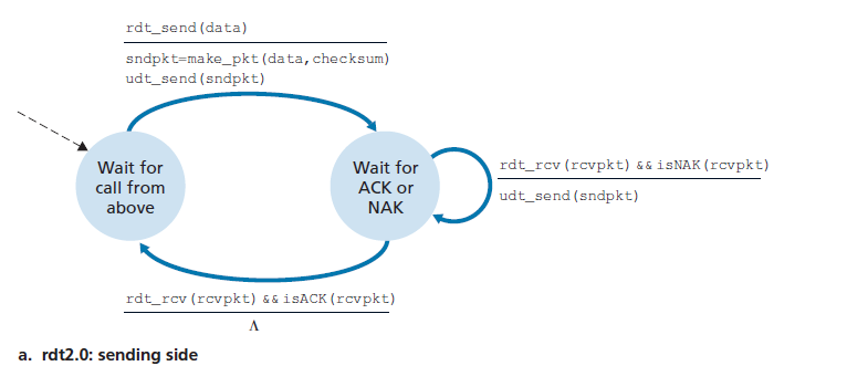
where there are two states: waiting for data to be passed down from the upper layer; waiting for ACK or NAK
- when
rdt_send(data)event occurs:- the sender will create a packet (
sndpkt) containing the data to be sent, along with a packet checksum - send the packet via the
udt_send(sndpkt)operation - transition to the rightmost state: waiting for an ACK or a NAK packet from the receiver.
- the sender will create a packet (
- when sender received response and it is
ACK, i.e.rdt_rcv(rcvpkt) && isACK(rcvpkt)- the sender knows that the most recently transmitted packet has been received correctly and thus the protocol returns to the state of waiting for data from the upper layer. Nothing needs to be done $\Lambda$.
- If a
NAKis received:- the protocol retransmits the last packet and waits for an ACK or NAK to be returned by the receiver in response to the retransmitted data packet
Blocking
- It is important to note that when the sender is in the wait-for-ACK-or-NAK state, it cannot get more data from the upper layer; that is, the
rdt_send()event cannot occur; that will happen only after the sender receives an ACK and leaves this state.- therefore, it is called stop-and-wait protocols
On the receiver’s side:
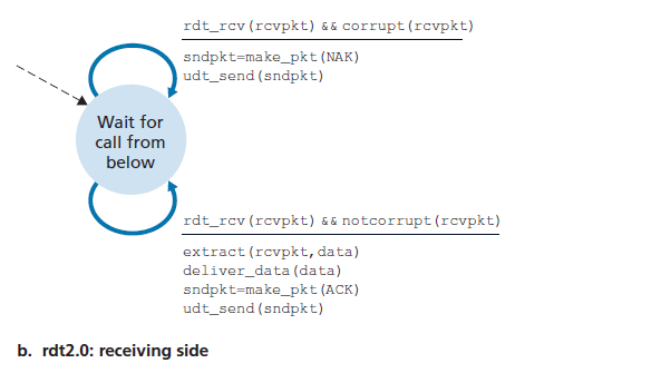
basically here the idea is simple. There is just one state as you just need to reply with either an ACK or a NAK
- if the data is not corrupt, send back
ACKand deliver the data to the application layer - if the data is corrupt, send back
NAKand do NOT deliver the data to the application
Feedback Corrupted: RDT2.1
Now, there is an additional problem. What if the ACK/NAK packet is corrupted in RDT2.0.
In specific, we will use the checksum, and add an additional field of sequence number
- if
ACKbecomesNAK, then you send a duplicate message (which might strew up receiver). In this case, you can:- sender add a sequence number to each packet
- receiver can now look at the sequence number and discard the duplicate
- receiver sends back
ACKagain
- if
NAKbecomesACK, but the checksum is wrong, you still resend the packet.- if something is wrong with the feedback, just resend the packet
- so that you are safe on not missing a packet, until you receive a correct/uncorrupted
ACK
Therefore, the state transition becomes, for the sender
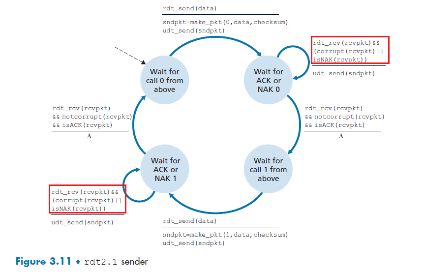
where here we just need 2 sequence numbers to disambiguate each packet, sequence number 0 or 1 (in this case)
- if the received packet is corrupt, we just resend the most recent packet for safety
- we transition to the next state $\iff$ feedback is not corrupt AND it is
ACK.
The receiver now does:
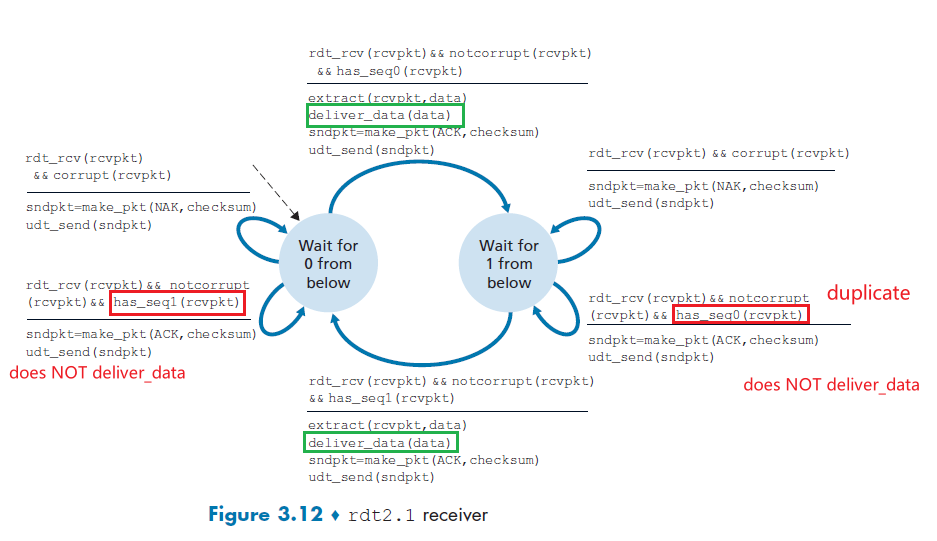
where notice that, for the receiver to resend a feedback packet, we now have two scenarios:
- the packet from sender is corrupt, send
NAK - the feedback I sent is corrupt, so now I get a duplicate. Then try to send
ACKagain.- Since the sender knows that a received
ACKorNAKpacket (whether garbled or not) was generated in response to its most recently transmitted data packet,ACKandNAKpackets do NOT themselves need to indicate the sequence number
- Since the sender knows that a received
Summary
At sender:
- sequence number is added (so that receiver can find duplicates)
- a 1-bit sequence number will suffice here, since it will allow the receiver to know whether the sender is resending the previously transmitted packet or a new one
- must check if received
ACK/NAKcorrupted- twice as many states
- state must “remember” whether “expected” pkt should have seq # of 0 or 1
At receiver:
- must check if received packet is duplicate
- state indicates whether 0 or 1 is expected pkt seq #
- note: receiver can not know if its last ACK/NAK received OK at sender
- i.e. the only way a receiver knows if an
ACKis received is that a sender gives the next packet. But if you are at the last packet from the sender, there is no next packet.
NAK-Free: RDT2.2
There is another way to deal with corrupted data, which is (actually closer to how TCP gets implemented): receiver sends `ACK` for last correct pkt received.
-
A sender that receives two ACKs for the same packet (that is, receives duplicate ACKs) knows that the receiver did not correctly receive the packet following the packet that is being ACKed twice
-
i.e. duplicate
ACKat sender results in same action asNAK: retransmit current pkt
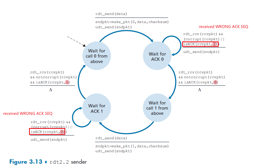
where the only difference with RDT2.1 is that:
- receiver added a
SEQto theACKpacket. So now the check is on if the latest correctACK SEQis up to date. If not, for example the bottom left, then it means aNAK. - note that again, we are assuming no packet loss can happen yet, so it is only about packet corruption.
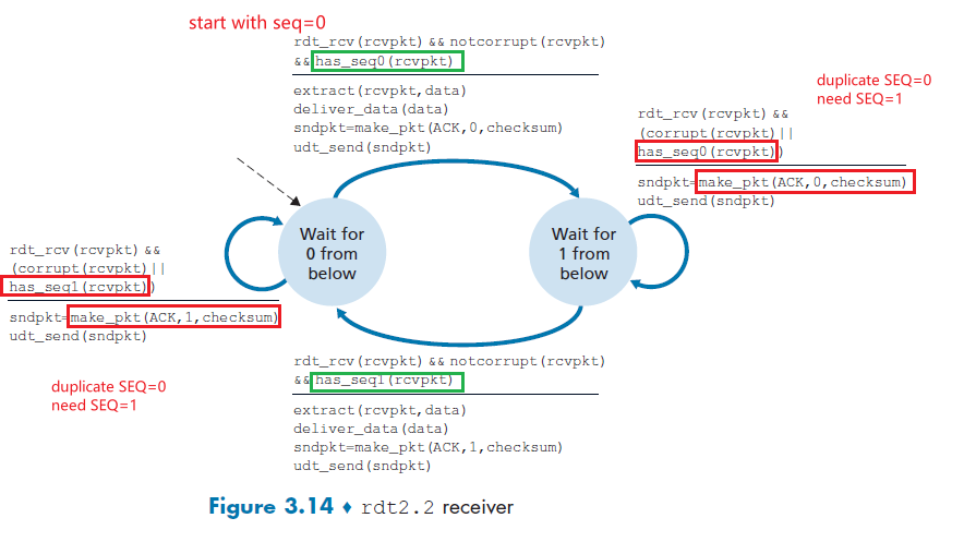
where:
- receiver must now include the sequence number of the packet being acknowledged by an ACK message (this is done by including the
ACK, 0orACK, 1)
Error and Loss: RDT3.0
Now we need to also deal with packet loss. This is a problem in our previous setup, since we had stop and wait. If a packet such as ACK is lost, then e.g. the sender will wait forever. Therefore, we have two additional tasks to fulfill:
- how to detect packet loss (this cannot be handled in RDT2.2)
- what to do when packet loss occurs (this in fact can be handled by RDT2.2)
Here, we assume that we are using the NAK-Free Protocol.
Idea
Here, we’ll put the burden of detecting and recovering from lost packets on the sender.
- Sender waits for a “reasonable” amount of time for
ACK. So that
- If either the data packet sent is lost, or the receiver’s ACK of that packet is lost, you get no response
- in that case, you just time out
- if it is just delayed too much, then you retransmit anyway (duplicate packet).
- This is the same as
NAK/ACKis corrupted, receiver can handle duplicates anyway in RDT 2.2.- Receiver doesn’t change much
- since if the data packet is loss, it never received it anyway. The sender will eventually resend it
- if there are duplicates, it is the same as RDT2.2
For sender
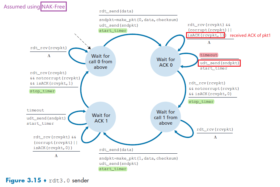
then basically:
- if the data and the
ACK/NAKare all correct, then you just get start and stop timers - expect
ACK, 1, but receiver sendsACK, 0or vice versa- we do nothing because, if the timer waiting for
ACK,0timed out before receiving any response, so we resent. But then we received the firstACK,0and proceeded to send packet 1. Then there would still be anACK,0on the way = 2ACK,0due to timed out + resend.
- we do nothing because, if the timer waiting for
- if the sender
timeout, then basically feedback is lost/delayed too much- either sender packet is lost, never reached receiver, or
ACKreply is lost - in any case, you retransmit
- either sender packet is lost, never reached receiver, or
Receiver
-
an exercise. Solution found online
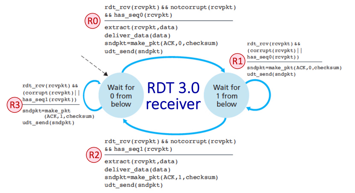
Note that
This means we need to decide on how long must the sender wait to be certain that something has been lost. Technically, this should be at least one round trip. But that has a problem of:
- the value differs link to link, time to time
- difficult to measure
- wasted bandwidth for just waiting that data
From the sender’s viewpoint, retransmission is a panacea.
- The sender does not know whether a data packet was lost, an ACK was lost, or if the packet or ACK was simply overly delayed.
RDT3.0: Timeline
Again, we are using the NAK-Free protocol.
When nothing went wrong:
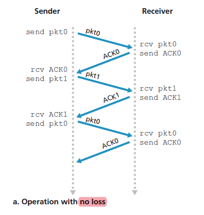
When you have a packet loss:
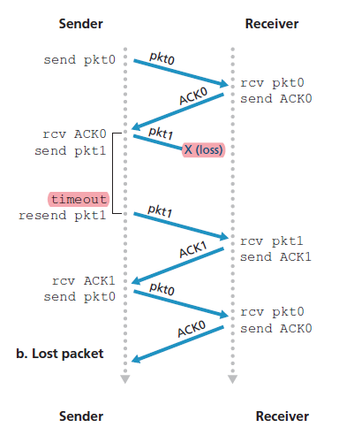
When you have a ACK loss:
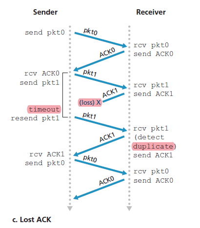
When your timeout is premature:
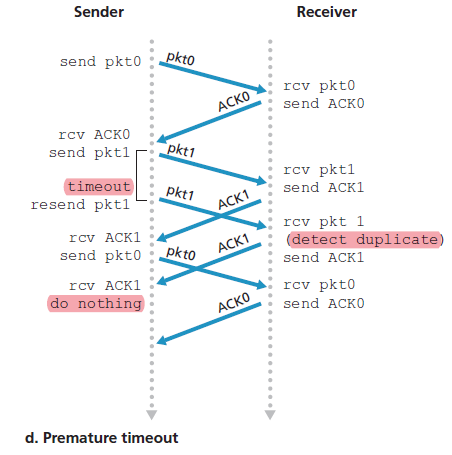
where the last case you do nothing because you have transmitted pkt0 just now. You are waiting for ACK0 already.
Stop-and-Wait vs Pipelining
Protocol rdt3.0 is a functionally correct protocol, but it is unlikely that anyone would be happy with its performance.
Suppose we have two hosts, and the setup is:
- propagation delay is $0.5\text{RTT}\equiv 15\text{ms}$ (assuming now processing delay, no queuing delay)
- transmission delay at sender is $L_s/R\equiv 0.008\text{ms}$ (e.g $R$, of 1 Gbps and $L_s$ is 1,000 bytes)
- transmission delay at receiver is $\approx 0$ since
ACKpackets are small
Then, the timeline of a normal RDT3.0 looks like, without any error:
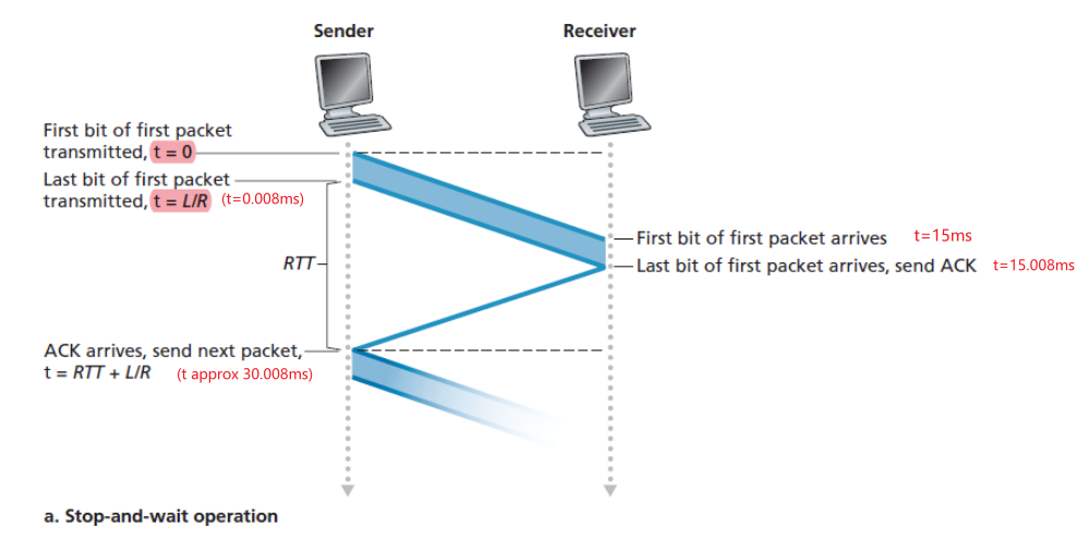
where if you calculate the utilization of the sender’s link, we basically only used $0.008$ millisecond out of $30.008$ second.
\[U_{\text{sender}} = \frac{L/R}{RTT+L/R} = \frac{0.008}{30.008}=0.00027\]Viewed another way, the sender was able to send only 1,000 bytes in $30.008$ milliseconds, an effective throughput of only $267$ kbps.
Utilization Time
The utilization of the sender (or the channel) as the fraction of time the sender is actually busy sending bits into the channel.
The solution to this is simple: Rather than operate in a stop-and-wait manner, the sender is allowed to send multiple packets without waiting for acknowledgments.
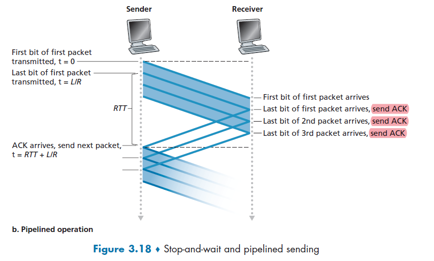
note that more than 3 packets can be send simultaneously. This is just an illustration.
Pipelining
Sender now sends multiple, “in-flight”, yet to be acknowledged packets sequentially. Receiver can also send multiple
ACKs.
- then, you are basically still sending while waiting. Saves time!
But this means that you need:
- your sequence number therefore has to increase (
0and1does not work)
- each in-transit packet (not counting retransmissions) must have a unique sequence number
- sender and receiver sides of the protocols may have to buffer more than one packet
- sender: buffer packets that have been transmitted but not yet acknowledged
- receiver: buffer out-of-order packets. (see Go-Back-N and Selective Repeat)
To implement the above, realize that there is a relationship between range of sequence numbers needed and the buffering requirements. In reality, there are two approaches:
- Go-Back-N
- Selective Repeat
Go-Back-N (GBN)
Basically, sender is constrained to have no more than some maximum allowable number, $N$, of unacknowledged packets in the pipeline.
- this limit $N$ will be then used for flow control. If that is not needed, we don't even need a limit here.
In the sender’s view of range of sequence number used in a GBN protocol (for buffering and resending):
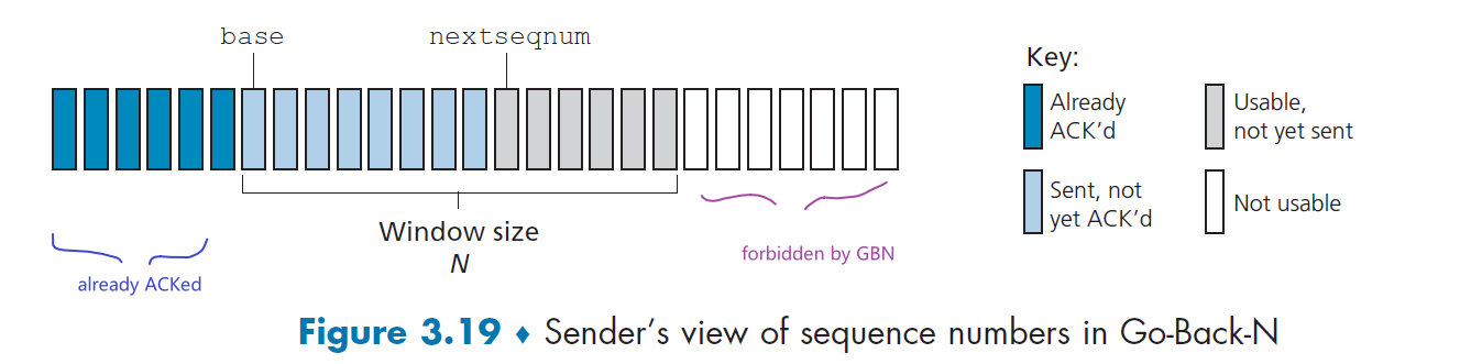
where we defined:
-
base: sequence number of the oldest unacknowledged packet -
nextseqnum: smallest unused sequence number -
therefore, we get four intervals:
- $[0,\text{base}-1]$ transmitted and acknowledged
- $[\text{base}, \text{nextseqnum}-1]$ transmitted but not yet acknowledged
- $[\text{nextseqnum}, \text{base}+N-1]$ packets to be transmitted immediately (if there are)
- $[\text{base}+N,\infty]$ forbidden region for GBN, must wait for one more acknowledgement from the window
note that technically, sequence number can only go up to $2^k$ for a field of $k$ bits. So you loop around when you reached $2^k$.
As the protocol operates, this window slides forward over the sequence number space. For this reason, $N$ is often referred to as thew window size and the GBN protocol itself as a sliding-window protocol.
Therefore, the FSM for sender looks like:
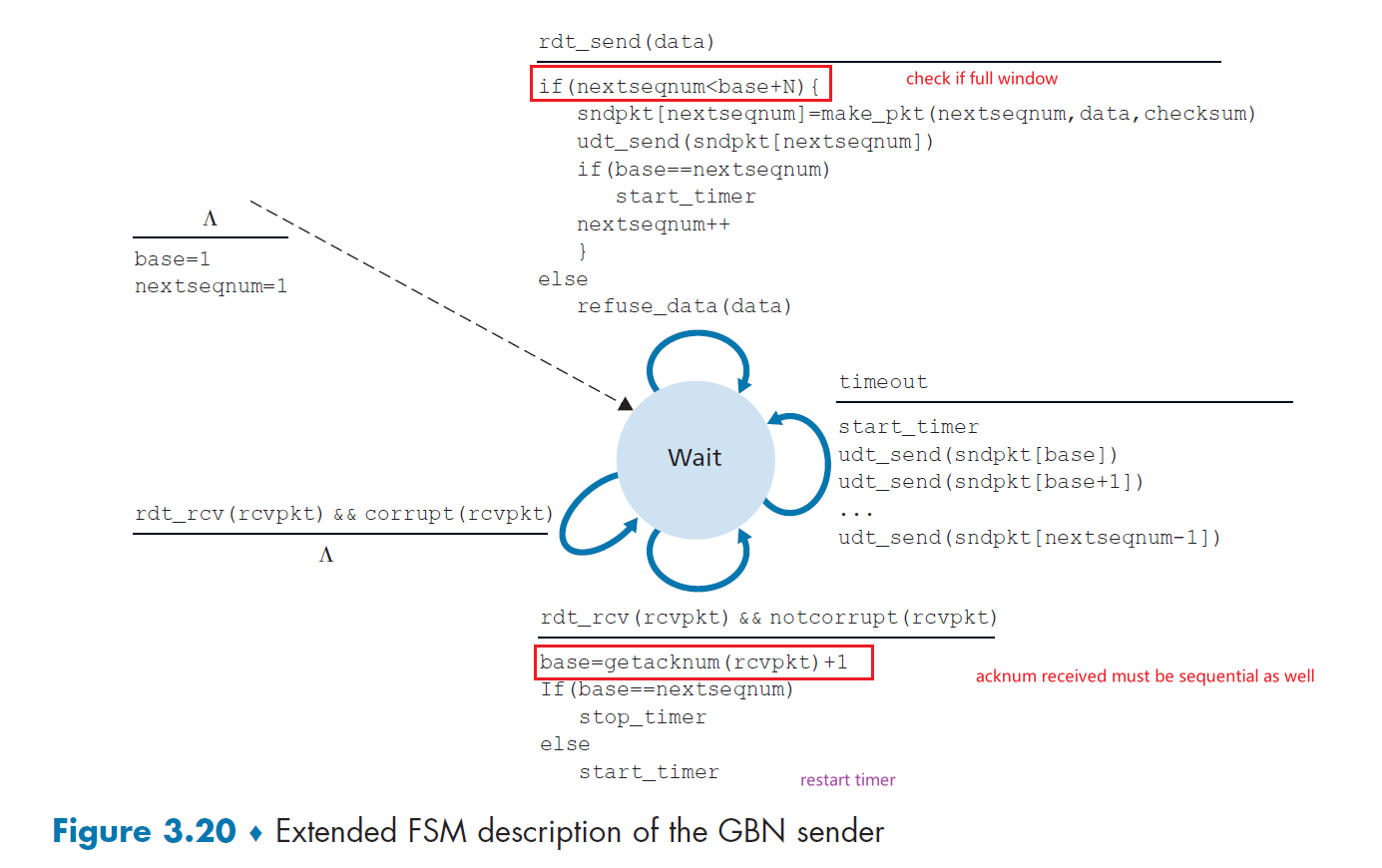
where notice that:
- Receipt of an ACK. In our GBN protocol, an acknowledgment for a packet with sequence number $n$ will be taken to be a cumulative acknowledgment, indicating that all packets with a sequence number up to and including $n$ have been correctly received at the receiver (check receiver side implementation to see how it works)
- A timeout event. timer will again be used to recover from lost data or acknowledgment packets. If a timeout occurs, the sender resends all packets that have been previously sent but that have not yet been acknowledged.
- basically, retransmit everything in the current window
- if there is a duplicate
ACK, ignore it
Timer in Sender GBN:
- basically can be thought of as a timer for the oldest transmitted but not yet acknowledged packet
For receiver:
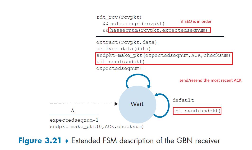
where:
- If a packet with sequence number $n$ is received correctly and is in order, then we deliver the data to APP and send
ACK - otherwise, discard the packet and send most recent `ACK` (we are in the
NAK-free protocol). This made sure that the use of cumulative acknowledgments is a natural choice for GBN.- as a result, you will send duplicate
ACK - alternatively, you could buffer out of order packets. But there is no need here.
- as a result, you will send duplicate
Therefore, for the receiver, the sequence number space looks like:
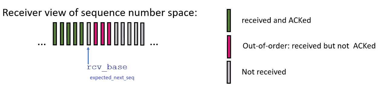
In Summary
- basically, the only exchange of “state” information between sender and receiver is the cumulative
ACK- this is simple to implement
- GBN is inefficient as it resend all $N$ packets in my window. For example, you received seq
1,2,5,6,7, then you will give a cumulativeACKof2. So eventually, all packets3,4,5,6,7will be retransmitted.
For a timeline series, GBN looks like:
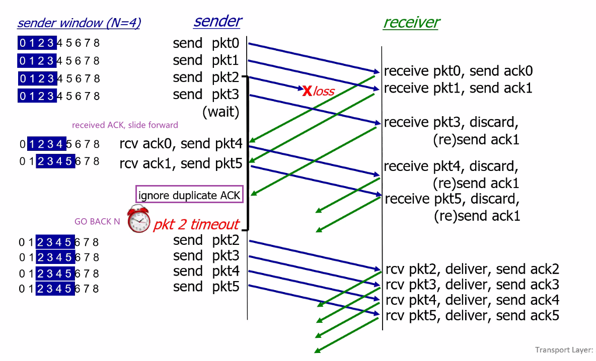
where alternatively:
- instead of ignoring duplicate
ACK, sender could immediately retransmit the missing ones - instead of discarding the out-of-order packets, receiver could buffer it
Selective Repeat (SR)
The problem with GBN was:
- A single packet error can thus cause GBN to retransmit a large number of packets, many unnecessarily (if receiver buffered)
Hence, selective-repeat protocols avoid unnecessary retransmissions by having the sender retransmit only those packets that it suspects were received in error. This means that:
-
still has a window size of $N$, start of window = first unACKed/unreceived message in the sequence
- now, both receiver and sender must have buffers
- sender has multiple timers, each individually for unACKed packets
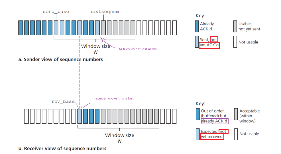
then for sender:
- Data received from above. Basically same as GBN, you check if it is within your window, and send only when it is within the window
- Timeout. each packet must now have its own logical timer, since only a single packet will be transmitted on timeout.
- ACK Received. The sender marks that packet as having been received, provided it is in the window. If the packet’s sequence number is equal to
send_base, the window base is moved forward to the next unacknowledged packet (basically the cumulative thing holds)
For receiver
- Packet with sequence number in $[\text{rcv_base}, \text{rcv_base}+N-1]$ is correctly received. Then the correctively received packets’
ACKare returned to sender. If the packet’s sequence number is equal torcv_baseis moved forward to the next unreceived packet. - Packet with sequence number in $[\text{rcv_base}-N, \text{rcv_base}-1]$ is correctly received. In this case, an `ACK ` for that old packet must be generated, even though this is a packet that the receiver has previously acknowledged. (otherwise the sender won’t go forward)
- e.g. you can receive past packet by a) your
ACKsimply got lost; b) basically sender timer timed out but yourACKreceived (delayed) right afterwards. In either case the receiver will have window moving forward already
- e.g. you can receive past packet by a) your
- Otherwise. Ignore.
Note
One important aspect of SR is that we have a lack of synchronization between sender and receiver windows. This will cause the following problem if we chose the wrong window size, as shown in Dilemma with Selective Repeat.
Basically, the upshot is that you need your range of sequence number to be at least twice of the windows size.
Time Series Example
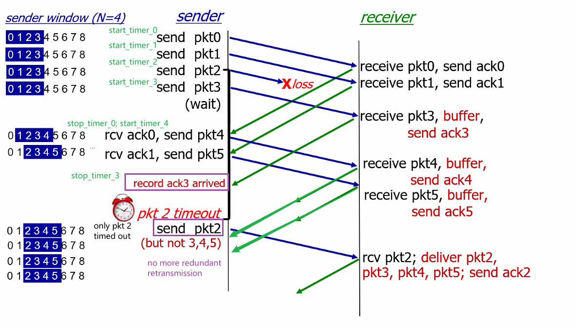
where after the ACK2 arrives, the sender will then shift the window all the way to packet base=6
Dilemma with Selective Repeat
Consider the case hat you have a window size of $3$, and your sequence number field is $2$ bits. So you only have sequence $0,1,2,3$. Now, consider the two scenarios:
| No problem | Problem |
|---|---|
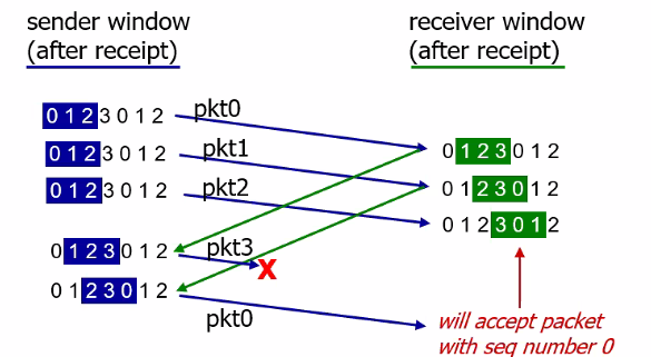 |
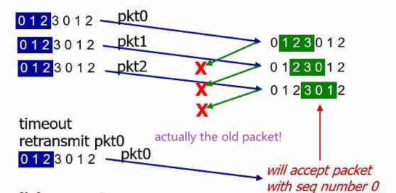 |
So from the receiver’s point of view, this looks like:
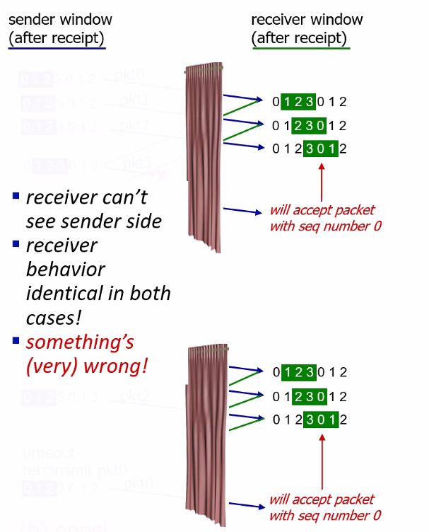
This happened because the window size is smaller than the sequence size (see figure below). The solution is to keep your sequence number $2N$ and above, for $N$ being window size.
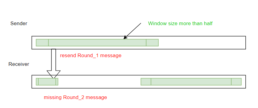
- so even if the problem case (which is the worst) happened, there is no overlap between the two windows in sequence number. Otherwise the receiver has no idea it the above is the next round of message or retransmission.
Take Away Message
Selective repeat is basically a better version than GBN, but it added complexity of:
- needs a wider range of sequence bits $\ge 2N$
- needs timer for each packet
- more processing on both receiver and sender side
GBN vs SR Model
Consider a simple model where:
- any packet transmission from sender is lost with probability, $p$
- ACKs never lost
We assume that each packet is independent.
Therefore, for Selective Repeat, it is simple. Recall that:
- sender knows exactly what receiver needs
Therefore, each pkt can be “examined” in isolation. Let $T_{SR}$ is the number of transmissions of one packet. Then:
\[\begin{align*} P[T_{SR} > i] &= P[T_{SR} = i+1] + P[T_{SR} = i+2]...\\ &= p^{i}[(1-p) + p(1-p) + p^2(1-p) + ...]\\ &= p^i (1-p)[1+p+p^2+...]\\ &= p^i (1-p)\frac{1}{1-p}\\ &= p^i \end{align*}\]Therefore, the average number of transmissions we need to do is:
\[\begin{align*} \mathbb{E}[T_{SR}] &= P(T_{SR}=1) + 2P(T_{SR}=2) + 3P(T_{SR}=3) + ...\\ &= P(T_{SR}>0) + P(T_{SR}>1) + P(T_{SR}>2) + ...\\ &= \frac{1}{1-p} \end{align*}\]For Go-back-N, recall that
- each round, sender transmits block of $N$ packets
- receiver informs sender of 1st lost pkt
- sender sends $N$ packets starting at 1st point of loss
- receiver dumps any packet in window after a loss.
$S_N$= # pkts arriving in receiver before a loss occurred in window of $N$ (successful transmission). Then, for $0 \le i < N$:
\[\begin{align*} P[S_{N} > i] &= P[S_{N} = i+1] + P[S_{N} = i+2]...\\ &= (1-p)^{i+1} \end{align*}\]basically at least the first $i+1$ packet is successfully transmitted.
Then the
\[\begin{align*} \mathbb{E}[S_{N}] &= P(S_{N}=1) + 2P(S_{N}=2) + ...+NP(S_{N} = N)\\ &= P(S_{N}>0) + P(S_{N}>1) + ... + P(S_{N}>N-1)\\ &= \frac{1-p-(1-p)^{N+1}}{p}\\ &= \frac{1-p}{p}(1-(1-p)^N) \end{align*}\]Notice that, plotting in desmos shows you that:
\[\lim_{p \to 0}\frac{1-p}{p}(1-(1-p)^N) = N\]Then let there be $m$ rounds of transmission, that we slide the window $m$ times. Since the window size is $N$:
\[\mathbb{E}[T_{GBN}]= \frac{\sum_{j=1}^mN}{\sum_{j=1}^mS_{N,j}}=\frac{\sum_{j=1}^mN/m}{\sum_{j=1}^mS_{N,j}/m}\]where $S_{N,j}$ be the number of packets accepted in the j-th round of transmission ($j$-th window slide).
- Notice that every time when a packet is lost, $S_{N,j} < N$ so our number of messages transmitted is larger than $1$.
Then, note that, since each round of transmission is independent:
\[\lim_{m\to \infty}\frac{1}{m}\sum_{j=1}^mS_{N,j} = \mathbb{E}[S_N]\]this is because we are taking the mean of successful transmission in each round, then with the law of large numbers, we get the expected value. Similarly:
\[\lim_{m\to \infty}\frac{1}{m}\sum_{j=1}^mN= N\]Hence we get:
\[\mathbb{E}[T_{GBN}] = \frac{Np}{1-p-(1-p)^{N+1}}\]Finally, graphing this, we can plot:
\[\frac{\text{average tranmission per packet in GBN}}{\text{average tranmission per packet in SR}} = \frac{\mathbb{E}[T_{GBN}]}{\mathbb{E}[T_{SR}]}\]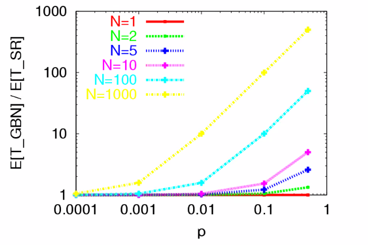
note that:
-
if the probability of packet loss increases, GBN needs to retransmit much more. Note that when the probability of loss is small $p\approx 0$, then the ratio is $1$, i.e. not much difference in performance
-
if we increase the window size, then Go-Back-N does worse and worse since chance of a packet being lost is higher
Summary
| Mechanism | Use, Comments |
|---|---|
| Checksum | Used to detect bit errors in a transmitted packet. |
| Timer | Used to timeout/retransmit a packet, possibly because the packet (or its ACK) was lost within the channel. Because timeouts can occur when a packet is delayed but not lost (premature timeout), or when a packet has been received by the receiver but the receiver-to-sender ACK has been lost, duplicate copies of a packet may be received by a receiver. |
| Sequence number | Used for sequential numbering of packets of data flowing from sender to receiver. Gaps in the sequence numbers of received packets allow the receiver to detect a lost packet. Packets with duplicate sequence numbers allow the receiver to detect duplicate copies of a packet. |
Acknowledgment ACK |
Used by the receiver to tell the sender that a packet or set of packets has been received correctly. |
NAK |
Used by the receiver to tell the sender that a packet has not been received correctly. Negative acknowledgments will typically carry the sequence number of the packet that was not received correctly |
| Window, pipelining | By allowing multiple packets to be transmitted but not yet acknowledged, sender utilization can be increased over a stop-and-wait mode of operation. Window size can further be set on the basis of the receiver’s ability to receive and buffer messages, or the level of congestion in the network, or both (see next chapter). |
TCP
Now that we have covered the underlying principles of reliable data transfer, let’s turn to TCP—the Internet’s transport-layer, connection-oriented, reliable transport protocol.
The TCP Connection
Recall that some properties of a TCP connection is:
- connection-oriented, because before one application process can begin to send data to another, the two processes must first “handshake” with each other (with the aim of initialize many TCP state variables)
- point-to-point, that is, between a single sender and a single receiver
- full-duplex service: If there is a TCP connection between Process A on one host and Process B on another host, then application-layer data can flow from Process A to Process B at the same time as application-layer data flows from Process B to Process A.
Now, let’s look at the basics of how a connection is established. Recall that we start with a client initiating the connection with:
clientSocket.connect((serverName,serverPort))
the above basically results in:
- the client first sends a special TCP segment informing the server
- the server responds with a special TCP segment as well
- the third segment is then sent from client to host again, which may or may not carry payload
Because three segments are sent between the two hosts, this connection-establishment procedure is often referred to as a three-way handshake. (which will be discussed in detail later)
After the connection is established, we basically send data with:
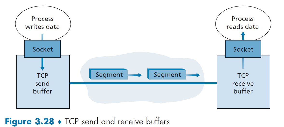
where basically:
-
the client application process pass data throughout the socket
-
then data is in the hands of TCP running in the client, which is directed into a send buffer (initialized during handshake)
-
From time to time, TCP will grab chunks of data from the send buffer and add a TCP header, thereby forming TCP segments.
-
The maximum amount of data that can be grabbed and placed in a segment is limited by the maximum segment size (MSS). This is set to ensure that a TCP segment (when encapsulated in an IP datagram) plus the TCP/IP header length (typically 40 bytes) will fit into a single link-layer frame.
Note that the MSS is the maximum amount of application-layer data in the segment, not the maximum size of the TCP segment including headers.
-
-
segments are passed down to the network layer
-
at the other end, the segment’s data is placed in the TCP connection’s receive buffer, and TCP would extract packets from that
-
Finally, the receiver application reads data from there
Take-Away Message
- a TCP connection consists of buffers, variables, and a socket connection to a process in one host, and another set in another host.
- No buffers or variables are allocated to the connection in the network elements (routers, switches, and repeaters) between the hosts, since Transport Layer is only at the ends.
- It turns out that TCP uses cumulative ACKs, which is more similar to GBN. Yet in reality implementation will have buffers to cache out-of-order packets, so it also has features of SR.
TCP Segment Structure
Basically we have two parts:
- header fields
- data field - a chunk of application data whose size is limited by MSS
A TCP segment looks like the following:
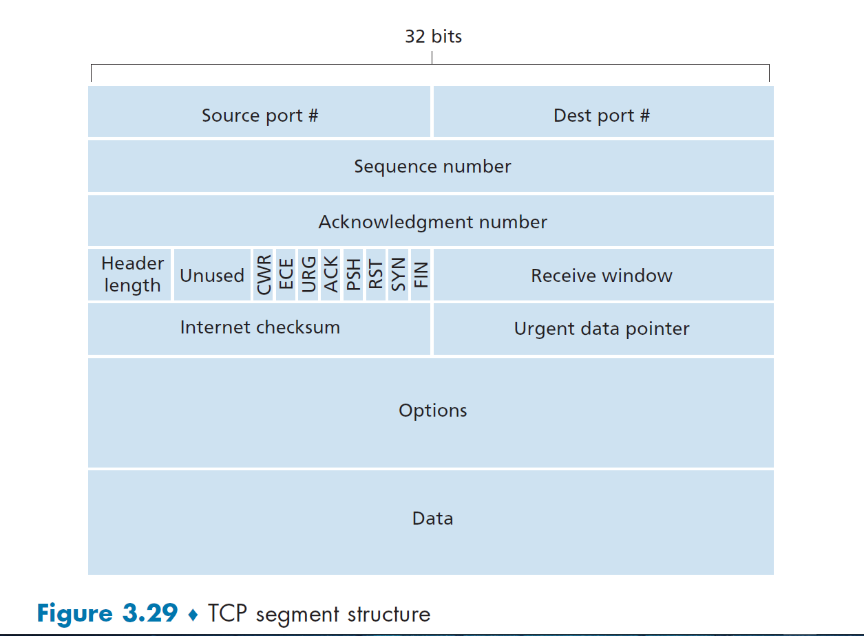
where we have:
- a source and destination port for multiplexing, and a checksum. This is the same for UDP as well.
- 32-bit sequence number field and the 32-bit acknowledgment number field, used for reliable delivery
- recall that we need 32 bit sequence number for pipelining
- the ACK number will be a cumulative ACK, which will be discussed below.
- we have both number, since this structure is used for all TCP segment/packets.
- 16-bit receive window field is used for flow control - number of bytes that a receiver is willing to accept
- restrict the size of window for total number of unacknowledged packets. This is depending on your device/network performance.
- 4-bit header length field specifies the length of the TCP header - variable length due to the TCP options field
- optional and variable-length options field is used when a sender and receiver negotiate the maximum segment size (MSS) or as a window scaling factor for use in high-speed networks.
- the flag field contains 6 bits. Basically:
ACKbit is used to indicate that the value carried in the acknowledgment field is valid, i.e. this segment containsACK.RST,SYN, andFINbit is used for connection setup and teardownCWR, andECEbits are used in congestion notificationPSHbit indicates that the receiver should pass the data to the upper layer immediatelyURGbit indicate there is urgent data
- 16-bit urgent data pointer field indicates the location of the last byte of this urgent data if there is. In practice, TCP must inform the receiving-side upper-layer entity when urgent data exists and pass it a pointer to the end of the urgent data.
Sequence and Acknowledgement Number
Basically, consider Host A is sending data to Host B. In TCP:
- The sequence number for a segment is therefore the byte-stream number of the first byte in the segment.
- The acknowledgment number that Host A puts is the sequence number of the next byte Host A is expecting from Host B.
- therefore, it is cumulative ACK.
For Example
Consider you are host A and you have 500,000 bytes, that the MSS is 1,000 bytes. Therefore, you need 500 segments. Suppose the first byte of the data stream is numbered 0.
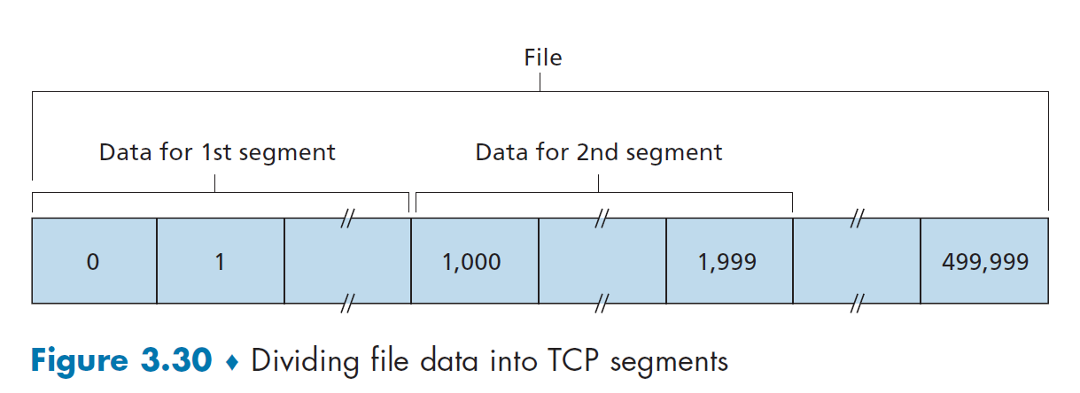
the sender Host A to B will have:
- The first segment gets assigned sequence number 0
- the second segment gets assigned sequence number 1,000
- the third segment gets assigned sequence number 2,000
- and so on
Note
- Here we assumed that initial sequence number start with $0$. In truth, both sides of a TCP connection randomly choose an initial sequence number. This is done to minimize the possibility that a segment that is still present in the network from an earlier, already-terminated connection.
Since Host A may be receiving data from Host B while it sends data to Host B. Suppose that Host A has received all bytes numbered 0 through 535 from B and suppose that it is about to send a segment to Host B.
- Host A puts $536$ in the acknowledgment number field of the segment it sends to B, which is the byte number host A is waiting for.
Out-of-Order
What if Host A received $0$ to $535$ AND $900$ to $1000$. Then technically there is no requirement on what to do, so it is programmer’s choice:
- discard the $900$ to $1000$ byte
- store it in the buffer, which is often used in reality for performance.
For Example: Telnet Login Shell
Suppose that A is trying to login B, so A initiates the connection as a client. The basic idea under a login shell is:
- user at the client type some character (not displayed on the screen yet),
- that character will be sent to the remote host
- remote host “echo back” the character is received and display it on the screen
- this is why you sometimes experience lag when typing in a remote
Now, suppose your client start with sequence number $42$, and the server start with sequence number $79$. Then:
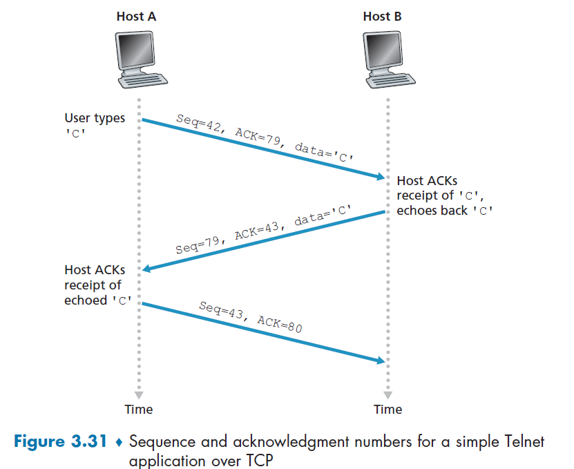
where:
- the first packet has
Seq=42because this is your first byte. It is expecting from serverSeq=79(i.e. next incoming byte should be placed at position $79 - \text{start seq}$) therefore it putAck=79. Finally, we are sending dataC, so that is in the payload. - the next packet is trivial, which is sent so that the client get something on the screen
- seq = 79, because server is telling client put `C` on the $79 - \text{server start seq}=0$th position of the buffer
- ack = 43, because server is expects/want to know what is the next data, which will be placed on the $43-\text{client start seq}=1$st position on the buffer
- the third segment has an empty data field, as its sole purpose is to acknowledge the data it has received from the server. Again the data design here is due to the implementation.
- even though there is no data, but because TCP has a sequence number field, the segment needs to have some sequence number
Round-Trip Time Estimation and Timeout
Now, we consider the TCP timeout that we had in our reliable delivery, which is needed basically for packet loss. In short, the consideration is:
- timeout needs to be longer than RTT, but RTT could vary
- timeout cannot be too short, resulting unnecessary retransmission
- timeout cannot be too long, resulting too slow reaction to loss
In reality, TCP determines this by first estimating the RTT value.
Estimating RTT
TCP sample some of its packet, measuring its `SampleRTT` for a segment: the amount of time between when the segment is sent (that is, passed to IP) and when an acknowledgment for the segment is received, i.e. its RTT.
- Instead of measuring a
SampleRTTfor every transmitted segment, most TCP implementations take only oneSampleRTTmeasurement at a time. That is, at any point in time, theSampleRTTis being estimated for only one of the transmitted but currently unacknowledged segments - Also, TCP never computes a
SampleRTTfor a segment that has been retransmitted
As a result, a new value for
SampleRTTis found approximately once every RTT time.
Since RTT will fluctuate, some sort of average is taken to compute EstimatedRTT:
basically the new EstimatedRTT is the weighted sum of the previous estimate and the new data.
- In statistics, such an average is called an exponential weighted moving average (EWMA).
Graphically:
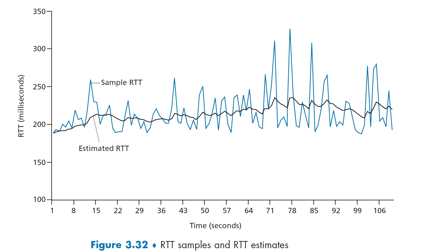
where pink would be our estimate, taking $\alpha=0.125$.
- however, we should not let timer be the `EstimatedRTT`, because then a lot of packets in the graph above would have timed out. Therefore, we need some measure of safety margin
where basically:
- this measures the variability of the RTT, so little fluctuation of
SampleRTTwill give small value forDevRTT - typically we take $\beta = 0.25$.
Finally, we then have:
\[\text{TimeoutInterval} = \text{EstimatedRTT} + 4\cdot \text{DevRTT}\]where an initial TimeoutInterval value of 1 second is recommended when there is no data in the beginning.
Note
when a timeout occurs, the value of
TimeoutIntervalis doubled to avoid a premature timeout occurring for a subsequent segment that will soon be acknowledged. The value is changed back after the segment is received.
- also, when
TimeoutIntervalis smaller than Real RTT, if we do not double the interval, then TCP will use previousTimeoutIntervalforever. Thus all packets will be retransmitted and no RTT mesurement happens.This timer for retransmission is often also called the Retranmission Timeout Value (RTO).
TCP Reliable Data Transfer
TCP creates a reliable data transfer service on top of IP’s unreliable best effort service.
In reality, TCP implements:
- use only a single retransmission timer, even if there are multiple transmitted but not yet acknowledged segments.
- though it is more effective to have one for each unacked packet in theory, it is a lot more overhead in practice
- recover technique from packet loss includes both timer and duplicate ACK, as you will seen soon.
TCP Sender
Basically, at sender we deal with three major events related to data transmission and retransmission.
Event: data received from application
- create segment with seq # (recall seq # is byte-stream number of first data byte)
- add the necessary fields in segment, as well as the data
- start timer if not already running
- think of timer as for oldest unACKed segment
- expiration interval:
TimeOutInterval
- pass the assembled segment to IP layer
Event: timeout
- retransmit segment that caused timeout (note this is different from GBN, which then retransmit all unacked packets)
- since there is only one timer, this makes it a bit inefficient if many consecutive packets are lost
- restart timer
event: ACK received
- if ACK acknowledges previously unACKed segments
- update what is known to be ACKed (starting from the
SendBaseof our sender window) - restart timer if there are still unACKed segments
- update what is known to be ACKed (starting from the
- otherwise, ignore or check Fast Retransmit
TCP Receiver
Here, the idea is to minimize the number of ACK, by trying to get cumulative ACKs.
| Event | TCP Action |
|---|---|
| Arrival of expected seq #. All previous ACK sent already. | delayed ACK. Wait for 500ms for next segment. If no segment, send ACK. |
| Arrival of expected seq #. One other segment hasn’t yet sent ACK | immediately send cumulative ACK, ACKing both segment. |
| Arrival of higher, out-of-order segment. | immediately send duplicate ACK, indicating seq. # for next expected byte |
| Arrival of segment that partially or completely fills in gap in received data. | Immediately send normal ACK, provided that segment starts at the lower end of gap. |
TCP Retransmissions
The following cases are bad, i.e. we have retranmissions:
| 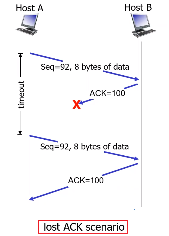 |
| 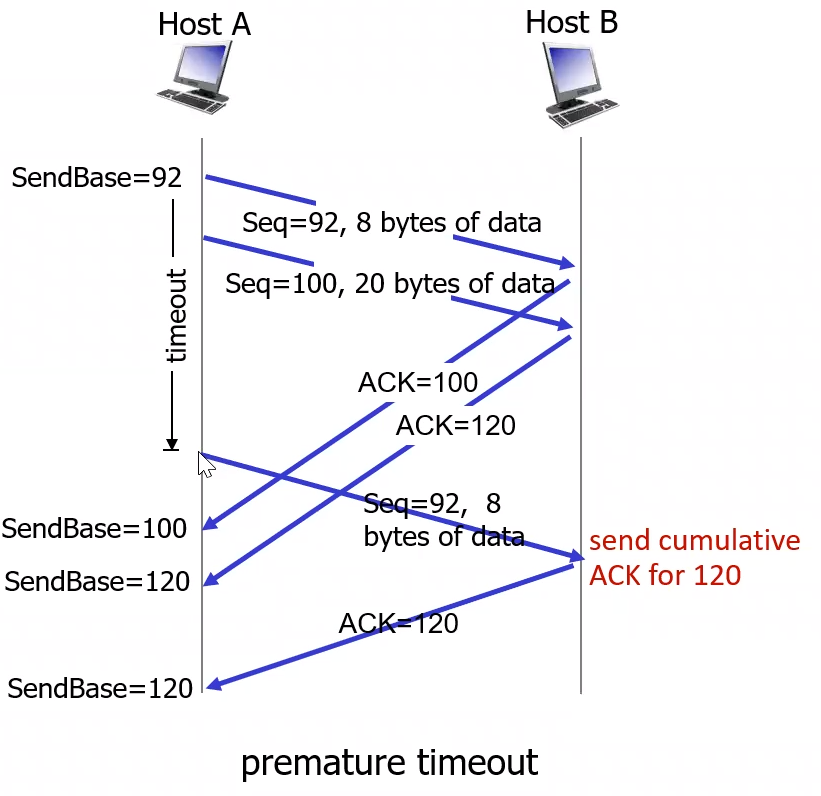 |
| :———————————————————-: | :———————————————————-: |
|
| :———————————————————-: | :———————————————————-: |
where on the left:
- when Host B receives the retransmission, it observes from the sequence number that the segment contains data that has already been received. Thus, TCP in Host B will discard the bytes in the retransmitted segment but still send the ACK.
On the right figure, when we have a premature timeout:
- Host A retransmit when timed out. It is interesting here to notice how the
SendBaseof Host A is updated throughout time.
Yet in this case, there is no retransmission:
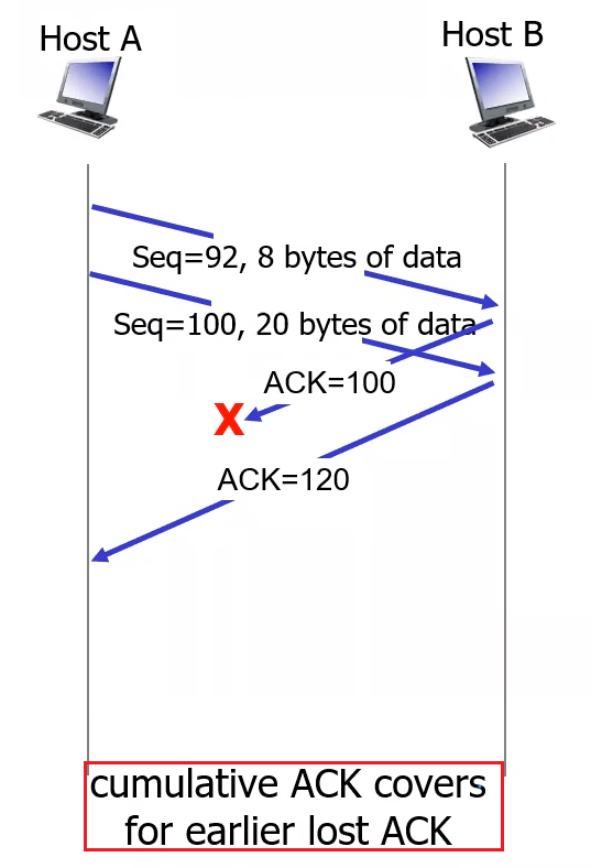
Note that in this case, there is no problem since we are using cumulative ACK:
- no timeout happened before the receipt of
ACK=120, so the sender updates it base to 120, and no retransmission is needed.
However, TCP gets smarter using the following techniques in addition. These are some modifications that is commonly used today.
Fast Retransmit
Consider the following case where a packet is lost
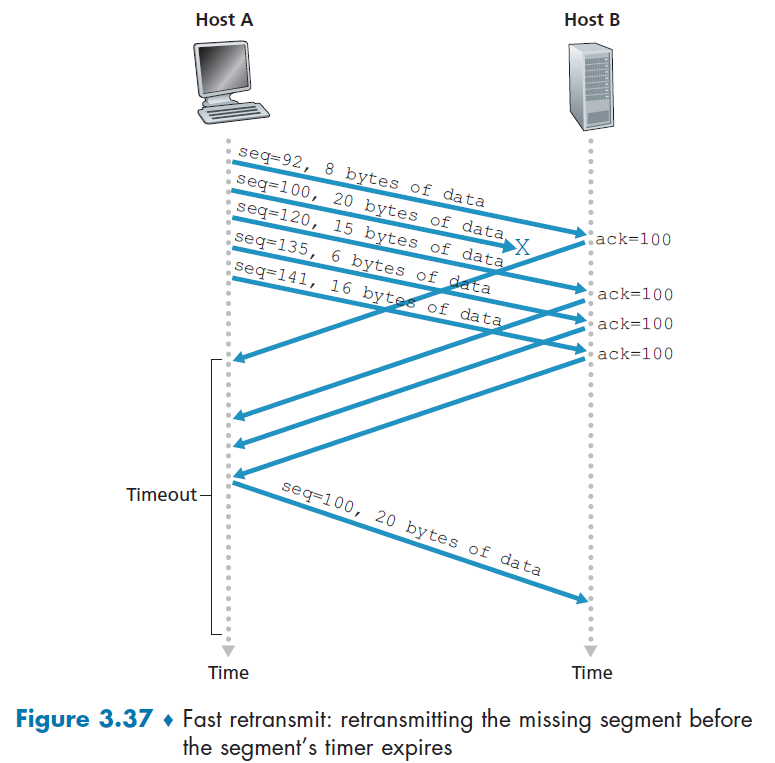
where the sender has received ACK=100 multiple times before timeout for seq=100:
- the sender has a high confidence that I have a lost packet. Therefore sender should retransmit now.
- in many practical implementation, we use triple duplicate ACK as a signal to initiate fast retransmit. (for Linux, it used double duplicate)
Doubling Timeout Interval
The idea is basically that, each time we timed out for a packet $X$, we double the TimeoutInterval from its previous value, without touching the computed estimate from $\text{TimeoutInterval} = \text{EstimatedRTT} + 4\cdot \text{DevRTT}$.
- the aim is to provide a from of congestion control: In times of congestion (e.g. ACK timeout perhaps due to it), if the sources continue to retransmit packets persistently, the congestion may get worse. The solution is to wait longer.
For Example
Suppose the timeout interval associated with the oldest transmitted yet unacked packet $X$ is $0.75$sec, which then expired.
- retransmit the packet, and set Timeout to be $1.75 \times 2 = 1.5$sec
- if still timed out, perform doubling again
Note that the above should not alter our most recent computation for $\text{TimeoutInterval}$, which TCP will continue with that computed value again once we received the ACK for packet $X$.
TCP Flow Control
Here the idea is that what if network layer delivers data faster than application layer consumes the data?
- recall that we have a receive buffer, which TCP place correctly received data for application to consume
- If the application is relatively slow at reading the data, the sender can very easily overflow the connection’s receive buffer
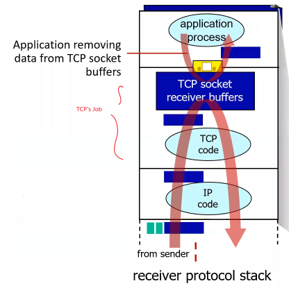
Note
- from the above it can be seen that each socket will have its own receive buffer. Therefore, demultiplexing in TCP just need to put the data into the correct buffer.
The solution is to use the receive window field in our segment:
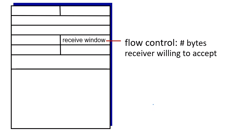
where:
- Informally, the receive window is used to give the sender an idea of how much free buffer space is available at the receiver.
- Because TCP is full-duplex, the sender at each side of the connection maintains a distinct receive window.
Hence, basically the value restored in the field is the value of rwnd:
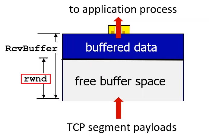
Now, suppose that Host A is sending data to Host B.
So that if we let variable in Host B be: LastByteRead being the number of bytes in the data stream consumed in the buffer by application; LastByteRcvd being the number of last byte that has arrived and placed in the buffer:
-
then
\[\text{RcvBuffer} \ge \text{LastByteRcvd} - \text{LastByteRead}\]RcvBuffertotal space must be:since TCP does not permit overflowing buffer.
In reality, this can be set in your program via options
RcvBuffer, and by default it is usually 4096 bytes.- many operating system will auto adjust
RcvBuffer
- many operating system will auto adjust
-
the receive window is
\[\text{rwnd} = \text{RcvBuffer} - (\text{LastByteRcvd} - \text{LastByteRead})\]rwndthe free space left in the buffer:
Therefore, Host B tells Host A how much spare room it has in the connection buffer, then what host A can do is to keep two variables: LastByteSend and LastByteAcked. Therefore:
-
the number of unacknowledged data byte is (notice it is in the unit of byte)
\[\text{LastByteSend} - \text{LastByteAcked}\] -
to keep no overflowing at Host B, Host A can make sure that:
\[\text{rwnd}_B \ge \text{LastByteSend} - \text{LastByteAcked}\]this is because we only have three cases for unacknowledged bytes:
- segment loss - doesn’t harm receiver’s buffer since its lost
- segment ACK hasn’t received - this actually goes into the buffer for host $B$
notice that only the second case we care, but that is exactly equal to the number of unacked bytes. Therefore, the above works.
TCP Connection Management
Recall that before exchanging data, we have some kind of handshake:
- agree to establish connection (each knowing the other willing to establish connection)
- agree on connection parameters (e.g., starting seq #s, which would be random)
- random seq number is useful for preventing spoofing and receiving packets from previous connections
On a high level, when the connection are established, we would have settled several variables such as seq #, which we need to decide during our handshaking procedure.
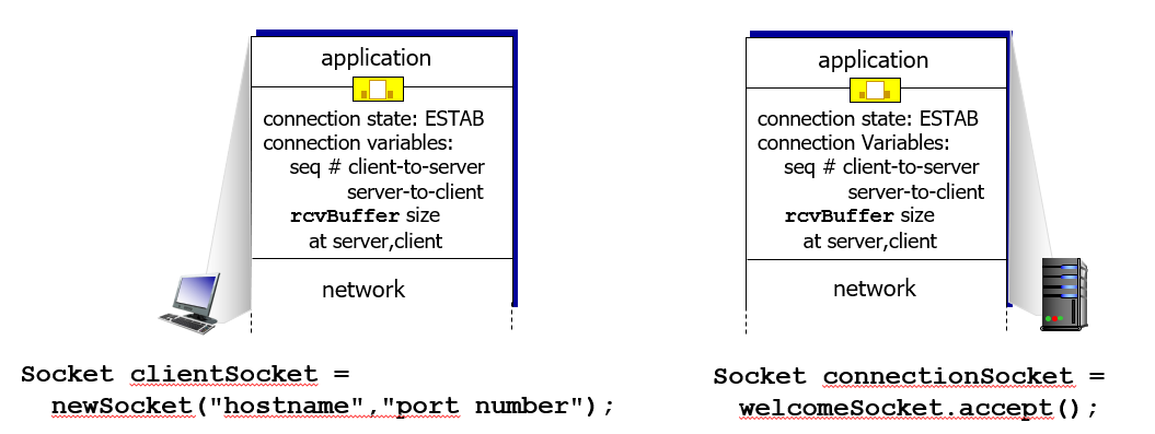
In general, there are multiple ways to do an establishment:
- 2 way handshake (problematic)
- 3 way handshake (used today)
2 Way Handshake
Consider having a 2 way handshake, so the idea is that:
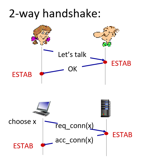
where the top half is the human analogy. This might seem to work, but in reality, consider the two cases:
-
Half Open Connection
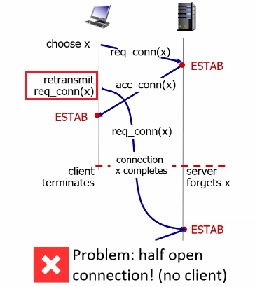
where basically:
- the client and server had a normal procedure of
ESTABusing two handshakes - yet it happens that client retransmitted the request connection `SYN`, such that it arrived after client termination
- then, the problem is that after termination, server receives a
SYNandESTABbut client has already terminated!
The upshot is that some resources at the server will then be wasted, which is actually used as a form of DOS attack to exhaust the server.
- the client and server had a normal procedure of
-
Duplicate Application Data
This is different from duplicate data due to packet losses, which can be solved using sequence number. Here it is a different issue.
Procedure What Server Sees After Termination 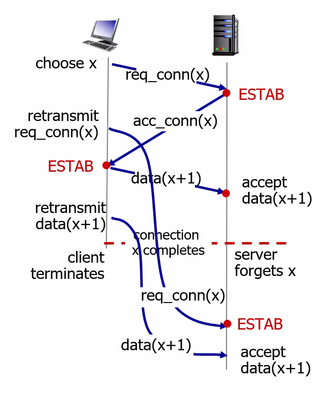
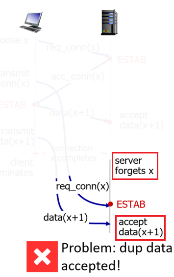
where notice that the procedure is basically:
- client happens to retransmit both the
SYNand some data which arrives after termination - however, the server sees the retransmission as a new connection with new data!
- client happens to retransmit both the
Take-Away Message
- the problem is that client is establishing the connection “too easily” to the server, that essentially it becomes a “one way handshake” for the client to trigger
ESTABon the server.
3 Way Handshake
Basically we have the following:
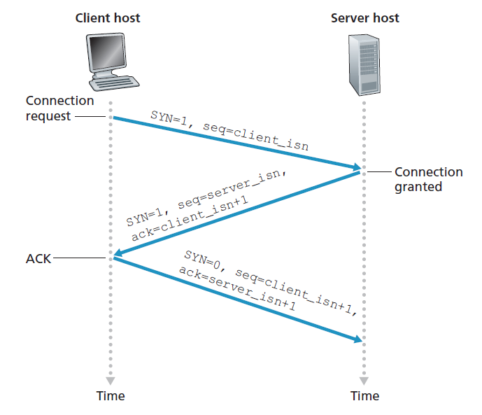
- client sends a special TCP segment - a `SYN` segment - to the server-side TCP. This special segment contains no application-layer data but a
SYNbit set to1. In addition, the client randomly selects a sequence numberclient_isn, and put it in the segment as well. - server replies back with a connection granted segment - a `SYNACK` segment, that basically says “I received your
SYNpacket to start a connection with your initial sequence number,client_isn. I agree to establish this connection. My own initial sequence number isserver_isn.” This is done by three header fieldsSYNbit set to1ACKset toclient_isn+1(and alsoACKbit is set to1since it contains anACK)- puts a randomly selected sequence number
server_isnin the sequence field
- client host then sends the server this last segment, which acknowledges the server’s connection-granted segment.
- note that the
SYNbit is set to0since connection is established now - techinically, this message can carry payload. This is why sometimes we see handshake takes $\approx$ 1 RTT.
- this makes the previous design of DOS attack not possible since the last
ACKfrom client will be dependent on the server’sSYNACK, which means it needs to read that message. Hence it is not possible to per-compose it before client termination.
- note that the
In a picture with more details:
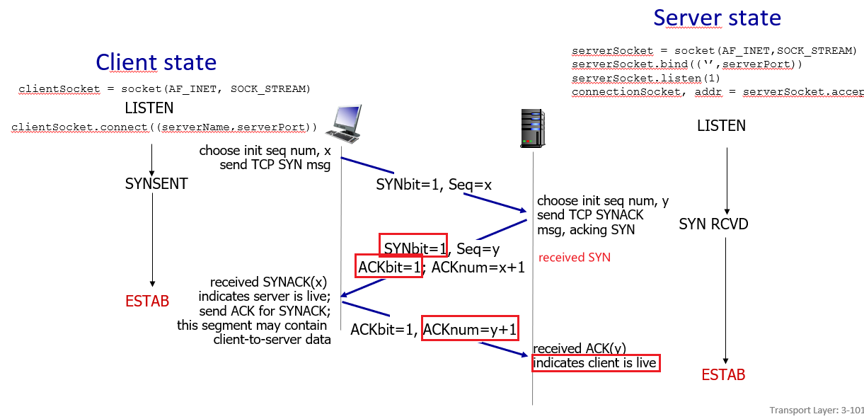
this is useful because it can solve hanging connection problem
- note that we used
SYNbit to start TCP connection
Closing TCP Connection
Basically we also have some kind of handshake, but here either of the two processes participating in a TCP connection can end.
For instance, suppose the client decides to close the connection
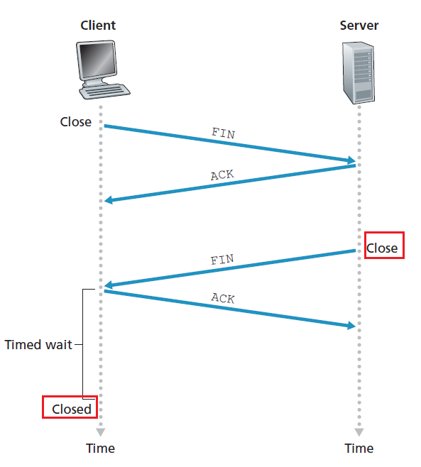
- client start a special segment with
FINbit = 1 - server respond to received
FINwith ACK- on receiving
FIN, ACK can be combined with ownFIN
- on receiving
- server then sends its own shutdown segment, which has the
FINbit set to 1 - client then replies with ACK
- at this point the client can deallocate resource
- but notice when the server/client is at the
CLOSEDstate
TCP States
Therefore, we could summarize all the above by using TCP states.
For client:
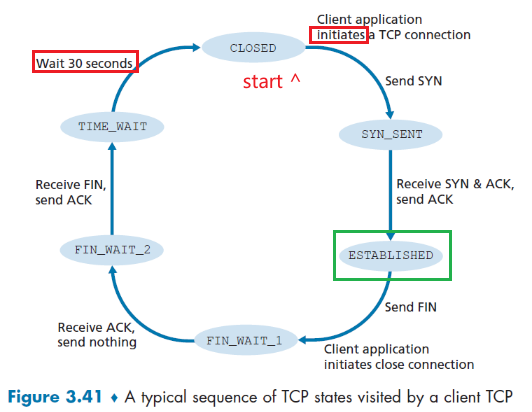
where basically you start with the CLOSED state, then:
- initiate a connection with the server by sending
SYN. (done by the creating theSocketobject in python) - While in the
SYN_SENTstate, the client TCP waits for theSYNACKsegment from the server- once received, it replies with an
ACK
- once received, it replies with an
- Then, once handshake completes, the client TCP enters the
ESTABLISHEDstate- this is when the TCP client can send and receive TCP segments containing payload
- Then, if the client wants to close the connection, it starts by sending
FIN=1segment and entersFIN_WAIT_1- this is when it waits for the
ACKfrom server for thatFIN
- this is when it waits for the
- When it receives the
ACKsegment, the client TCP enters theFIN_WAIT_2state- waiting for server to sendFIN=1.- once received, the client acknowledges the server’s segment and enters the
TIME_WAITstate
- once received, the client acknowledges the server’s segment and enters the
- The
TIME_WAITstate lets the TCP client resend the final acknowledgment in case the ACK is lost- the time for waiting is implementation-dependent, could be 30sec, 1min, etc.
- After the wait, connection formally closes and all resources is released at the client (e.g. port number)
For the server
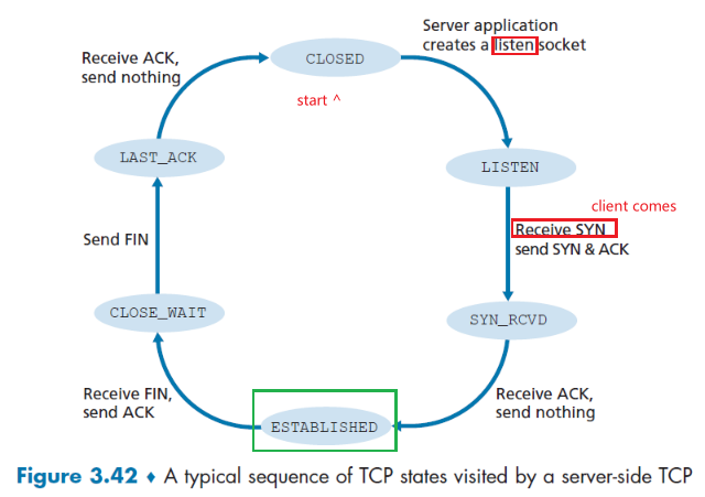
where here we are assuming the client initiated the tear down. Otherwise everything should be clear.
Note
- here we technically haven’t talked about if both sides of a connection want to initiate or shut down at the same time. Those issues are not covered here.
Yet one case you need to know is when, say the client sent a SYN segment to socket 80 (assume firewall lets it through), but no server socket is running on 80. Then, the host will send a special reset segment to the source/client. This TCP segment has the RST flag bit set to 1.
- this is basically saying “I don’t have a socket for that segment. Please do not resend the segment”
Alternatively, if the client didn’t receive any message, then it could mean that SYN segment was blocked by an intervening firewall and never reached the target host.
Principles of Congestion Control
Recall that
- in flow control, we were rate matching between the sender and the receiver, so that the receiver is not overwhelmed.
- in reliable data transfer where we designed retransmission (e.g. due to overflowing of router buffer), it solved the symptom of network congestion (i.e. packet loss) but didn’t solve network congestion itself.
Here, we are matching the speed of the sender and the network, by perhaps throttling the sender so that you don’t have too much:
- long delays (due to network congestion)
- packet loss (due to network congestion)
Task To Achieve
Too many sources sending too much data too fast for network to handle!
but we also need to utilize the network as much as possible!
The difficulty here is that:
- this thing needs to be scalable, since the network core could be very complicated
- high variation within the network
Causes and the Costs of Congestion
Here we begin by understanding the problem first: examine three scenarios in which congestion occurs.
In particular, we focus on what happens as hosts increase their transmission rate and the network becomes congested.
Scenario 1: Two Senders, a Router with Infinite Buffer
The setup is as follows:
- two senders $A$, and $B$, sending at the same rate of $\lambda_{in}$ bytes/sec
- router has infinite buffer, but a finite capacity of $R$
- the number of bytes/sec received at the receiver is $\lambda_{out}$
- assume no retransmission, no loss data, etc.
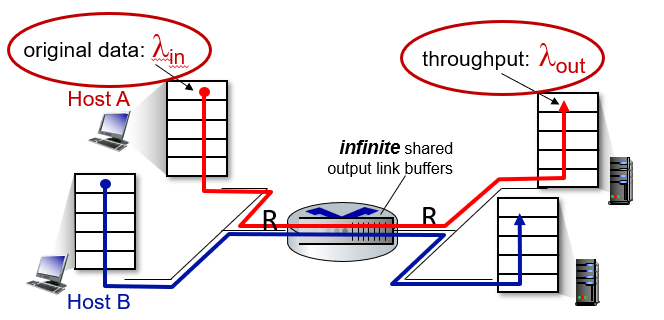
Then, if we measure the throughput, i.e. $\lambda_{out}$ as a function of $\lambda_{in}$ input, we see that:
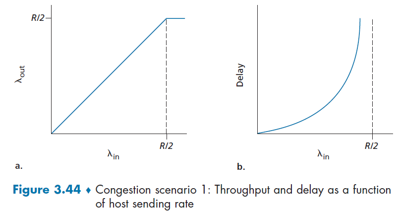
so:
- the left figure basically shows that the throughput is bounded at $R/2$
- but as throughput approaches $R/2$. the average delay will get huge!
Scenario 2: Two Senders and a Router of Finite Buffer
Now, we consider the same setup, but the modifications that:
- router has a finite buffer, so packet will get dropped when it has full buffer
- we are using reliable data delivery, so we will have retransmission
- hence while the application is sending at $\lambda_{in}$, TCP layer is actually sending at $\lambda_{in}’$ due to extra retransmission
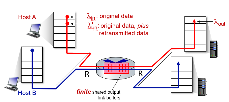
Then, the upshot is that determining $\lambda_{in}$ and throughput $\lambda_{out}$ depend strongly on how retransmission is performed.
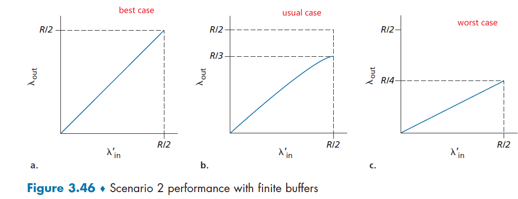
where :
- the best case we have Host A is able to somehow (magically!) determine whether or not a buffer is free in the router and thus sends a packet only when a buffer is free. In this case, no loss would occur
- more realistic case, e.g. we retransmit for 3 duplicate ACK or timeout. Then, when we have $\lambda_{in}’=0.5R$, the throughput is lower since some of the $0.5R$ will be duplicates.
- in this case, $\lambda’{in}=0.5R\to \lambda{out}=0.333R$. This means that $0.5R-0.333R\approx 0.166R$ are duplicate retransmissions
- the worst case is that every packet is retransmitted from the sender
Note
The upshot is that we will have both needed and unneeded (e.g. premature timeout) retransmissions, where arguably both needs to be taken into account/will affect the network.
So the Figure 3.46 b) could be:
where that unneeded retransmission is more annoying.
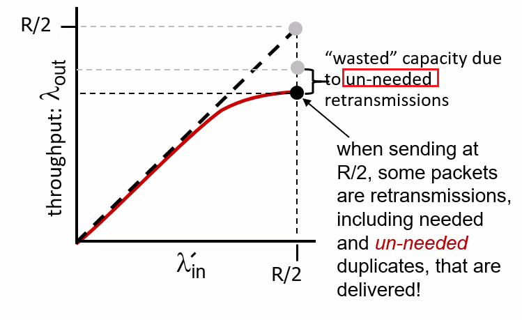
Scenario 3: Multi-hop Path
Here we:
- assume that we have RDT implemented
- all hosts intent to transmit at the same rate of $\lambda_{in}$
- all 4 routes have the same capacity of $R$, and a finite buffer
We have A sending to C, D sending to B over four routers
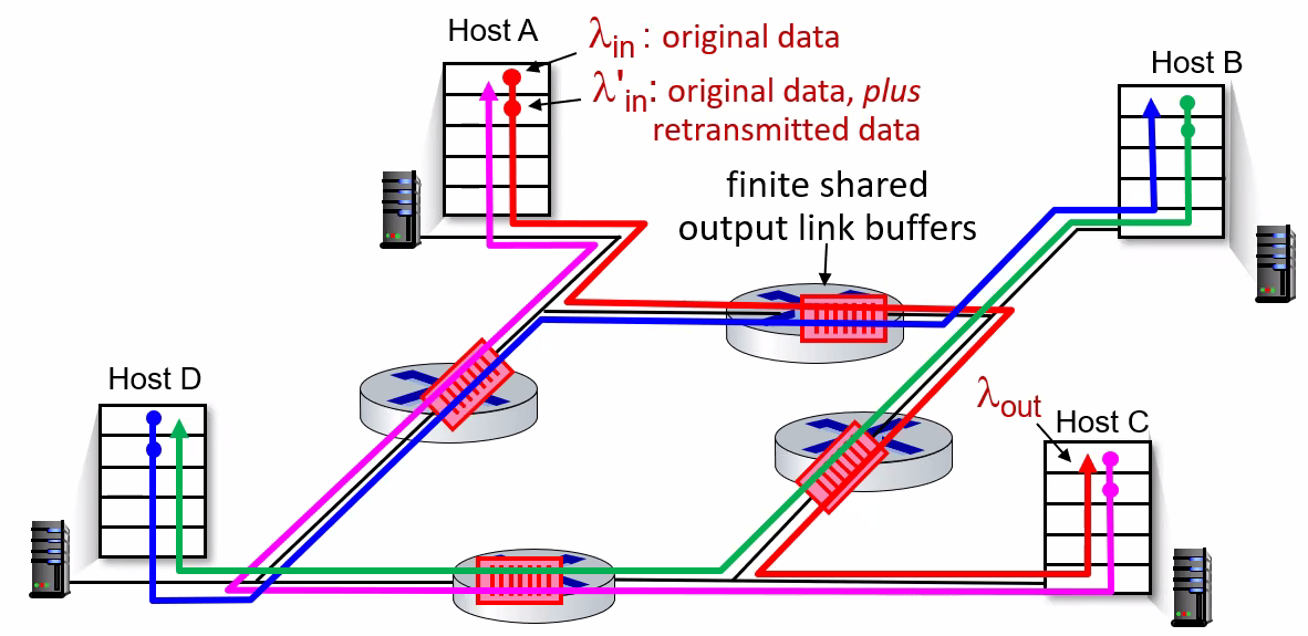
where notice that here we have another problem:
- the maximum capacity of each router becomes $R/2$ since it is shared
- consider if it happens that the GREEN packet is sending faster than $R/2$, then it piles up at RIGHT router
- since the RED packet from A-C also needs the RIGHT router, this will result in eventually no RED data arriving at host C, hence throughput of A-C will diminish!
- if A-C throughput diminishes, then it could be the same as the TOP router just dropping RED packets and remain IDLE = doing useless work! Basically it would be a waste of resource to even pick up red packets in this case.
Hence, in this unfortunate scenario, we get (e.g. for A-C in this case)
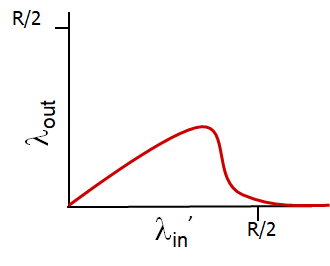
where:
- in the beginning when $\lambda_{in}$ is small, there is no competition
- as $\lambda_{in}’$ gets larger, competition happens and the multi-hop router basically becomes a disaster! It would be equivalent of router doing useless work!
Summary of Congestion Situations
| Take Away Message | Graph |
|---|---|
| throughput can never exceed capacity | 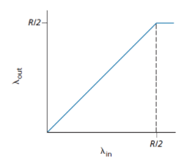 |
| §delay increases as capacity approached | 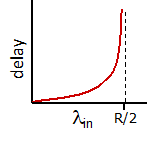 |
| loss/retransmission decreases effective throughput | 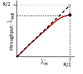 |
| un-needed duplicates further decreases effective throughput | 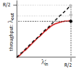 |
| upstream transmission capacity/buffering wasted for packets lost downstream | 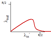 |
Up to this point, we discussed what it looks like for congestion to happen. Next we discuss how to fix/react to improve the situation.
TCP Congestion Control
Heuristics
In general there could be two solutions:
- End systems infer congestion by looking at packet delay and packet loss
- e.g. is delay is high or packet is loss, then it could be that the network is congested
- this is also called: End-to-end congestion control.
- Routers provides feedback to sender and receiver on current network status
- i.e. the network layer is providing some assistance
- the problem here is to make it scalable
- this is also called: Network-assisted congestion control
Classic TCP Congestion Control
here we cover the “classical” TCP —the version of TCP standardized in [RFC2581] and most recently [RFC 5681] — uses end-to-end congestion control rather than network-assisted congestion control.
In general, the idea is to answer the following to problems:
- how does TCP throttle the sender
- how does TCP perceive congestion
Throttling the Sender
This is done by TCP having an additional variable at the sender, which is cwnd - congestion control window. Such that:
where notice that the LHS is just unacknowledged data.
- in practise, the window size is exactly $N \equiv \min\{\text{cwnd}, \text{rwnd}\}$.
Now, if we assume that TCP receive buffer is so large that the receive-window constraint can be ignored; thus we only focus on cwnd, then approximately the sender sends at rate:
because basically:
- at the beginning of every RTT, the constraint permits the sender to send
cwndbytes of data into the connection - after roughly the end of RTT, you can send new round of
cwndbytes.
Graphically, your window size now is restricted by cwnd, so that you cannot send more than that:
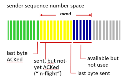
Perceiving the Congestion
Then the problem is to decide what `cwnd` we should take.
First, define that “loss event” at a TCP sender as the occurrence of either a timeout or the receipt of three duplicate ACKs from the receiver.
Then basically we have two scenarios:
- Congestion happens: We know that congestion will cause the loss event to happen, either due to large delay -> timeout, or to full buffer at router -> packet loss.
- decrease the
cwndwindow
- decrease the
- Everything is Good: we receive
ACKs as expected. So we can increase the congestion window size usingACKreceived- If
ACKarrives fast, thencwndincreases fast - if
ACKarrives slow, thencwndincreases slow
- If
Exactly what is the increasing rate and the decreasing rate of the cwnd window is implementation/algorithm dependent.
Take-Away Message
Situation Desired Action A lost segment - congestion TCP sender’s rate should be decreased when a segment is lost An ACKreceivedSender’s rate can be increased when an ACK arrives for a previously unacknowledged segment Therefore, the overall approach is to do some bandwidth probing
- adjusting its transmission rate is to increase its rate in response to arriving ACKs until a loss event occurs
TCP Congestion-Control Algorithms
The algorithm has three major components:
- slow start
- congestion avoidance
- fast recovery
In many different variants of the algorithm, Slow start and congestion avoidance are mandatory components, but the difference is in how they increase the size of cwnd in response to received ACKs.
Component: Slow Start
This describes the initial probing process when the sender knows nothing yet about the network.
-
the value of
cwndis typically initialized to a small value of 1 MSS. Therefore, the sending rate is approximately $\text{MSS}/\text{RTT}.$ -
the value of
cwndincreases by 1 MSS every time a transmitted segment is first acknowledged.- i.e. we have a exponential increase (not linear)
graphically, this looks like
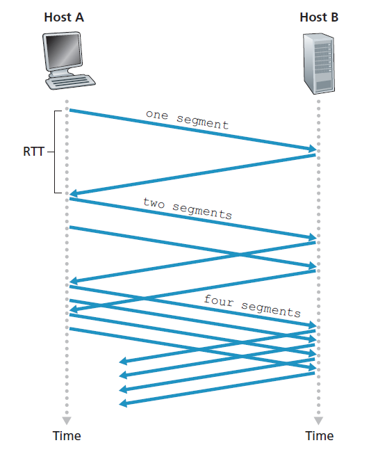
Now, slow start ends in the following three scenario:
- If a timeout event occurs, then it sets a variable
ssthreshto $\text{cwnd}/2$, which is half of the value ofcwndwhen the loss occurred. Then, setcwnd=1and start anew. - If
cwndget larger to equal tossthresh, it is not a good idea to continuous doubling so we switch to congestion avoidance, where you increase thecwndin a more cautious manner. - If three duplicate
ACKis received, then you perform a fast retransmit and switch to the fast recovery state.
Therefore, the full algorithm can be also summarized in the FSM:
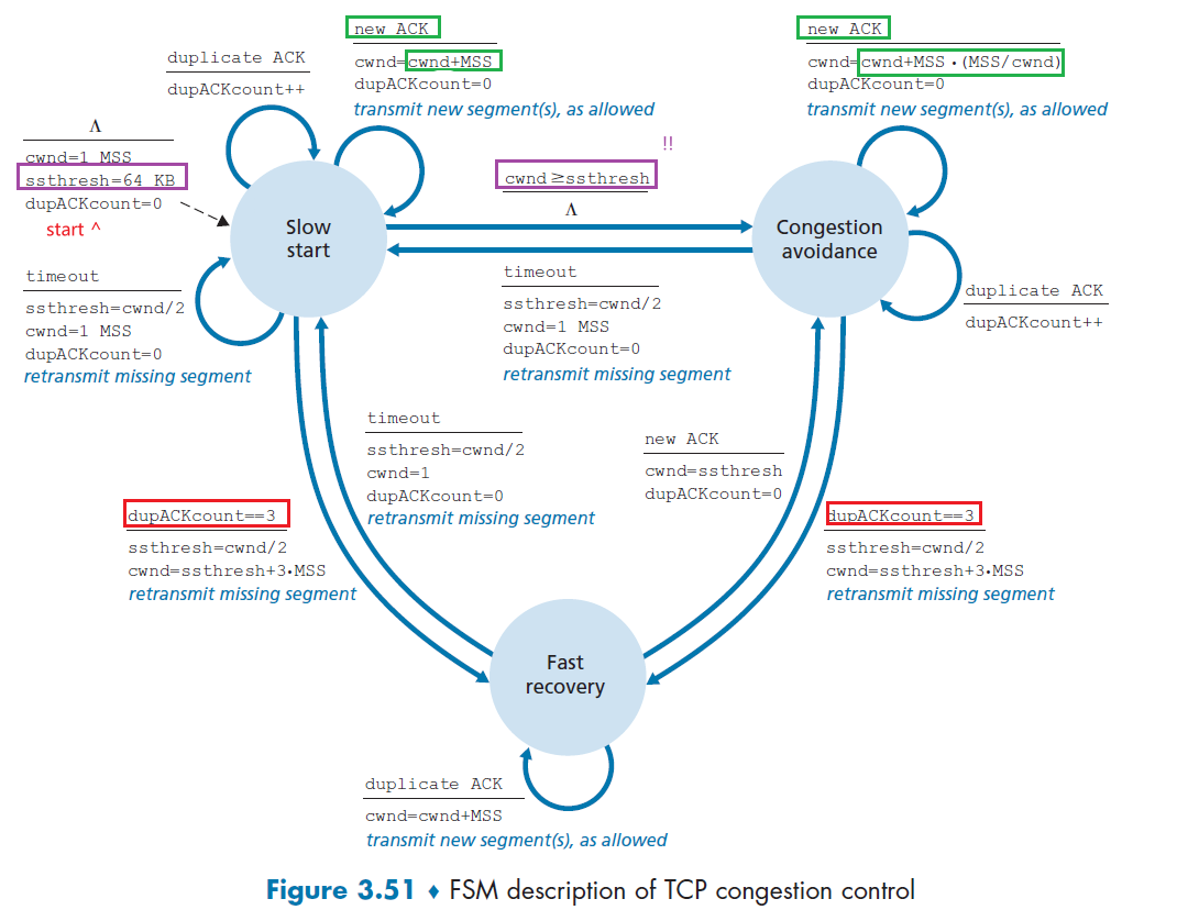
where you actually start with a non-zero ssthresh.
Component: Congestion Avoidance
Remember that on entry to the congestion-avoidance state, the value of `cwnd `is approximately half its value when congestion was last encountered. Congestion could be just around the corner!
Therefore, here we actually pursue a more conservative, linear increase by:
-
increases the value of
cwndby just a single MSS every RTT (instead of everyACK). The net result is you basically peform:cwnd += MSS * (MSS/cwnd)where notice that
(MSS/cwnd)is the same as 1 over the number of segments sent within an RTT -
the result is having an actual linear increase in
cwnd
Finally, this increase ends in a similar manner as the slow start:
-
a timeout occurs t: The value of
cwndis set to 1 MSS, and the value ofssthreshis updated to half the value ofcwndwhen the loss event occurred. (same as slow start) -
a triple duplicate
ACKoccurs, here it is different. Because this is at least an indication of the network is continuing to deliver some segments from sender to receiver, the reaction is less dramatic to a timeout.TCP halves the value of
cwnd(adding in 3 MSS for good measure to account for the triple duplicate ACKs received) and records the value ofssthreshto be half the value ofcwndwhen the triple duplicate ACKs were received.
Component: Fast Recovery
Here, the value of cwnd is increased by 1 MSS for every duplicate ACK received for the missing segment that caused TCP to enter fast-recovery.
Then a transition/recovery is done when:
- an normal ACK arrives for the missing segment, TCP enters back the congestion avoidance
- a timeout occurs, then fast recovery transitions to the slow-start state after performing the same actions as in slow start and congestion avoidance.
Note
- Fast recovery is a recommended, but not required, component of TCP
Example: TCP Tahoe and TCP Reno.
Basically Reno implemented the Fast Recovery, where Tahoe didn’t and just cuts the cwnd=1 every time when a timeout occurs.
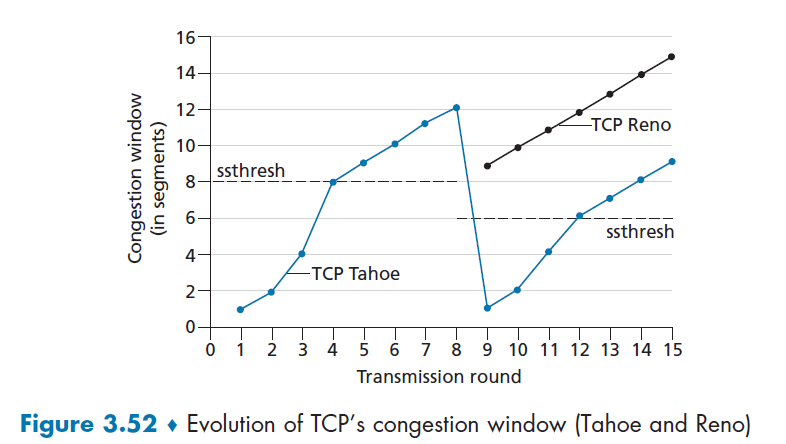
then, the comparison is shown here:
- in the beginning up to the 8-th tranmission round, performance is the same
- at the 4-th transmission, both entered congestion avoidance state.
- when at the 8-th transmission round, a loss (triple ACK) occurred, Tahoe cuts to
cwnd=1the next round while Reno has $0.5\cdot 12 + 3=9$ ascwndand then grows linearly.- both still has the
ssthreshto be $0.5 \cdot 12=6$. So Reno then immediately enters congestion avoidance
- both still has the
Summary: AIMD
The TCP congestion control algorithm can be summarized in the FSM
But additionally, if we ignore the initial slow start period and assuming losses is only triple duplicates (i.e. no timeouts, never went back to slow start), then you always are either increasing linearly or halving the cwnd:
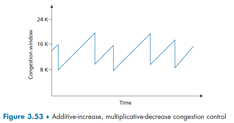
Therefore, TCP congestion control is often referred to as an additive-increase, multiplicative decrease (AIMD) form of congestion control.
Why AIMD works out in reality?
AIMD – a distributed, asynchronous algorithm – has been shown to:
there is almost no shared information needed across users, except perhaps for sharing the same multiplicate constant $\beta$
optimize congested flow rates network wide!
have desirable stability properties
Note
If we were to draw the performance graph, the one similar to economics
basically here we have two important lines:
- fairness line so the bandwidth is the same
- full utilization line
Then, what AIMD does is basically:
where we start with non-equable/efficient usage, but:
when we are probing, there is a multiplicative increase so the gradient is $1$.
- when overutilization occurs, we get $u_1/\beta, u_2/\beta$, for $\beta$ being the constant used in the multiplicate decrease, so that they go close to the line joining with point $0,0$
- eventually it oscillates towards the “best point”
- this works for $N$ dimensions, so it scales
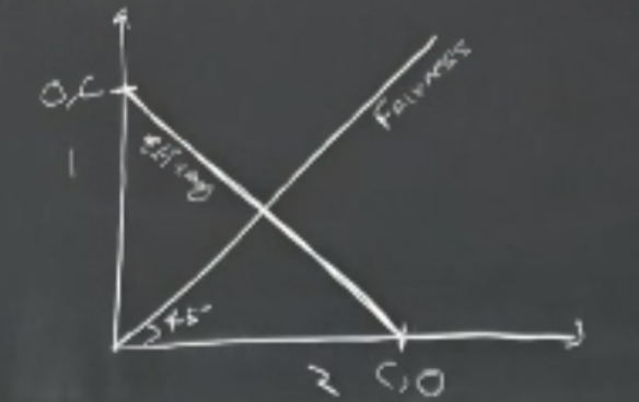
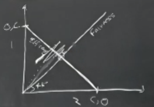
TCP CUBIC
This is another algorithm that slightly tweaks the classical implementation, and turns out to work better and gets used today most often.
Heuristics
- cutting the sending rate in half and increasing lineally could be overly cautious? Perhaps the linear increase part could be done quicker to utilize the internet more?
Graphically, CUBID does the same thing for slow start and fast recovery, but differs in congestion avoidance, resoling in:
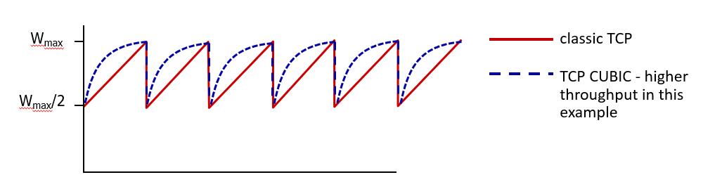
where:
- the area difference is the gain in network bandwidth.
- this is employed often in reality
In more details, it basically use a cubic increase instead of a linear increase. The idea is actually simple, so for congestion avoidance:
- Let $W_{max}$ be the TCP’s congestion
cwndwhen a loss is detected. Let $K$ be the estimated time you will reach another $W_{max}$ in the future. - CUMIC increases the congestion window as a function of $(t-K)^3$ (along with several tunable parameters)
- Since it is a cubic function, as $t$ exceeds $K$, CUBIC can more quickly find a new operating point if the congestion level of the link that caused loss has changed significantly
Graphically:
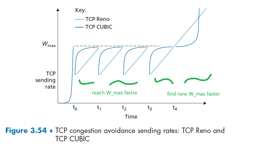
where, again assuming loss = triple duplicate:
- when $t < K$, the rate increases as $(t-K)^3$, hence reaches $W_{max}$ faster
- when it turns out $t > K$ and our network is still good, we want to find out the new limit. Cubic function increases/find it fast when the new congestion level has changed significantly.
Network Assisted and Delay-Based Algorithm
One problem with AIMD is that, we basically takes action when the packet is drop = after buffer is full. But what is perhaps better is to just be careful when buffer is about to be full, so we avoid packet loss which causes loss detection/recovery to take a long time.
- this is these are recent changes to the TCP algorithm when the network layer are revamped
- they basically either build on top of the AIMD principle we discussed before, both basically aims to detect congestion BEFORE packet loss occurs.
Explicit Congestion Notification
ECN basically lets routers use an
ECNbit to indicate congestion (close to full packet). Then the sender should treat thatECNthe same as a loss packet by reducing the window size to half - preventing from packet loss.
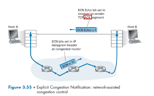
where, after a sender (Host A) sent something:
-
when a router along the path congested (about to be full), it sets the
ECNbit to 1 of all packets in the buffer in a probabilistic manner-
deciding on when a router “is congested” is implementation dependent
-
the first bit of
ECNis to inform routers whether if sender/receiver isECNcapable (TODO: not sure if true) -
the probabilistic maner means it sets all packets with
\[\frac{R}{N} =\frac{c}{\mathrm{RTT}\sqrt{p}}\]ECN=11with a probability of $p$ defined as:where:
- $R$ is the bandwidth it has, $N$ is the number of users using it. So $R/N$ is the ideal/fair throughput per user
- the RHS is the real life approximated throughput per user, with $p$ being the probability of packet loss, $c$ being some constant
- so the more the user $N$, the higher the computed $p$, the more packets will be marked with
ECN=11
-
-
when the receiver received the packet, if the
ECNis set to 1, it also sets theECE(explicit congestion echo) bit to 1 to inform the sender -
when the sender received the
ACKwithECE=1, it does a multiplicative decrease by halving the window (as if in fast retransmit)- the sender also sets the
CWR(Congestion Window Reduced) bit in the header of the next transmitted TCP sender-to-receiver segment
- the sender also sets the
Note
- this is network assisted because the router needs to do things: routers need to have the network layer/IP with the two bits
ECNset.- since we avoid packet losses, we could achieve a shorter overall delay as well (by avoiding costly packet loss and retransmission). So this principle is also employed in transport protocols used in Data Centers.
- this scales since router itself doesn’t need to do too much work.
Delay-Based Congestion Control
Similar to the above, the aim is to proactively detect congestion onset before packet loss occurs/full buffer. However, this is not network assisted, so everything is done at the sender.
Basically:
-
Sender measures the RTT of the source-to destination path for all acknowledged packets
-
compute the minimum $\mathrm{RTT}_\min$, which represents the case with low congestion and low queuing delay
-
compute the uncongested throughput rate to be:
\[\frac{\mathrm{cwnd}}{\mathrm{RTT}_\min}\] -
so if current throughput is close to that, increase your $\mathrm{cwnd}$, i.e. network is uncongested now. Otherwise, if it is significantly less than it, decrease the sending rate similarly by doing multiplicative decrease.
Fairness
First let us consider the world with TCP only.
Fairness
Suppose we have $K$ TCP connections, but all passing through a bottleneck link with transmission rate $R$ bps.
Then a control mechanism is said to be fair if the average transmission rate of each user is $R/K$.
We can illustrate the above concept in a 2D example that easily generalizes into $K$ dimension:
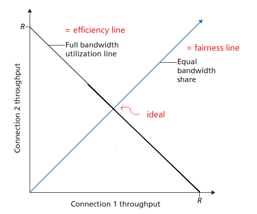
Now, let us investigate if the TCP algorithms covered above are fair/efficient.
TCP AIMD
Assume that we have two connections, and they have the same MSS and RTT (so that if they have the same congestion window size, then they have the same throughput). And suppose we ignore the slow start, such that they start at point $A$ in the graph below.
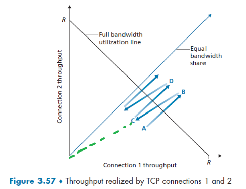
then notice that:
- when they are below the efficiency line, they do additive increase, each increase by 1 MSS = parallel to the $[1,1]^T$ vector.
- when they experience loss above the efficiency line, they do multiplicate decrease of reducing window size of half. Hence this basically is halving the $\vec{OB}$ vector.
After some iterations, AIMD will oscillate along the fairness line, so it is a fair algorithm in this condition.
Note
- This works iff the RTT is the same. In general, those sessions with a smaller RTT are able to grab the available bandwidth at that link more quickly as it becomes free. Hence client-server applications can thus obtain very unequal portions of link bandwidth.
Fairness and UDP
Many multimedia applications, such as Internet phone and video conferencing, often do not run over TCP for this very reason above. So they use UDP because they do not want their transmission rate throttled!
Now the question is, is UDP fair when we have both TCP and UDP?
The answer is no, because:
- When running over UDP, applications can pump their audio and video into the network at a constant rate (at the expense of occasionally lose packets)
- therefore, since UDP does not decrease transmission rate during congestion but TCP will, it is possible for UDP sources to crowd out TCP traffic.
(But luckily, there are a number of congestion-control mechanics that prevents UDP from taking over TCP.)
Fairness and Parallel TCP
Even if UDP gets to be forced to behave fairly, there is another way to “rob bandwidth”: using multiple parallel connections.
Therefore obviously this is not being fair as well and needs to be considered:
- suppose there were only two user, each has only one connection. Then with bottleneck router of bandwidth $R$, each user gets $R/2$
- A new user joins in but opens 2 parallel TCP connection. Now the router would give $R/4$ per connection! This gives the third user an overall $R/2$ bandwidth but the other 2 only $R/4$.
Evolving Transport Layer Functionality
Up to know we discussed mainly TCP and UDP.
Over times, we have identified circumstances in which neither is ideally suited, and so the design and implementation of transport layer functionality has continued to evolve.
For example:
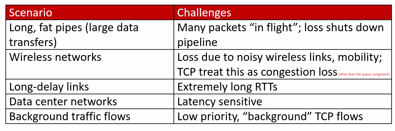
So over times, as we have seen before, there are many variations to a TCP protocol, and now perhaps the only common features of these protocols is that they use the TCP segment format.
QUIC: Quick UDP Internet Connections
This is an popular evolving protocol in place of TCP for HTTP. QUIC is a new application-layer protocol designed from the ground up to improve the performance of transport-layer services for secure HTTP.
- Google has deployed QUIC on many of its public-facing Web servers, in its mobile video streaming YouTube app, in its Chrome browser, etc.
- technically, QUIC is an application protocol, but it is interesting how it implements some features of TCP, and then use UDP for transport layer
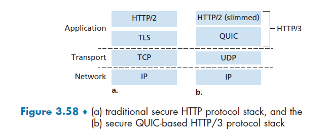
Some features of QUIC in the application layer include:
-
Connection-Oriented and Secure: now it basically does handshake in application layer, where it combines the handshake for connection establishment AND authentication + encryption (see Figure 3.58 (a)). Hence, it only needs to do one handshake, which speeds up the connection establishment procedure.
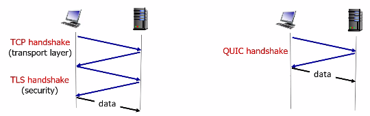
- Streams: QUIC allows several different application-level “streams” to be multiplexed through a single QUIC connection, and once a QUIC connection is established, new streams can be quickly added. This basically solves the Head of Line problem mentioned in HTTP 1.1.
- Each connection has a connection ID (established during the handshake), and each stream within a connection has a stream ID; both of these IDs are contained in a QUIC packet header
- Then, data from multiple streams may be contained within a single QUIC segment, which is carried over UDP.
- Hence, the separate streams also solves the HOL blocking when a packet is lost, i.e. in the HTTP1.1 case, all the other HTTP request packets are delayed/have to wait. However, with QUIC we have packers delivered per-stream basis, a lost UDP segment only impacts those streams whose data was carried in that segment; HTTP messages in other streams can continue to be received and delivered to the application.
- Reliable, TCP-friendly congestion control: QUIC provides reliable data transfer to each QUIC stream separately.
- Reliability is the same as TCP
ACKmechanism - Congestion control is based on TCP NewReno [RFC 6582] - a slight modification to the TCP Reno protocol (see Component: Fast Recovery)
- Reliability is the same as TCP
Overview of QUIC protocol architecture:
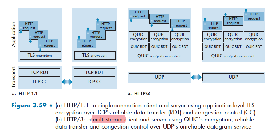
Finally, the advantage of application layer protocol is that changes can be made to QUIC at “application-update timescales,” that is, much faster than TCP or UDP update timescales.
Chapter 4 Network Layer: Data Plane
Now basically we deal with IP address: given a message, deliver a message from an IP address to another IP address
- in transport layer, it delivers from one port to another port
- in application layer, it delivers from one process to another process
Note
Remember that Physical, Link, Network Protocol is implemented on all devices, where as Transport and Application Layer is only on end devices.
Basically we want to discuss host-to-host communication service: how do packets go from one host to another.
The network layer is actually a complicated one, so we will cover it in two goes:
- data plane functions of the network layer — the per-router functions in the network layer that determine how a datagram (that is, a network-layer packet) arriving on one of a router’s input links is forwarded to one of that router’s output links.
- control plane functions of the network layer—the network-wide logic that controls how a datagram is routed among routers along an end-to-end path from the source host to the destination host
Overview
Also notice that now we are at the network core:
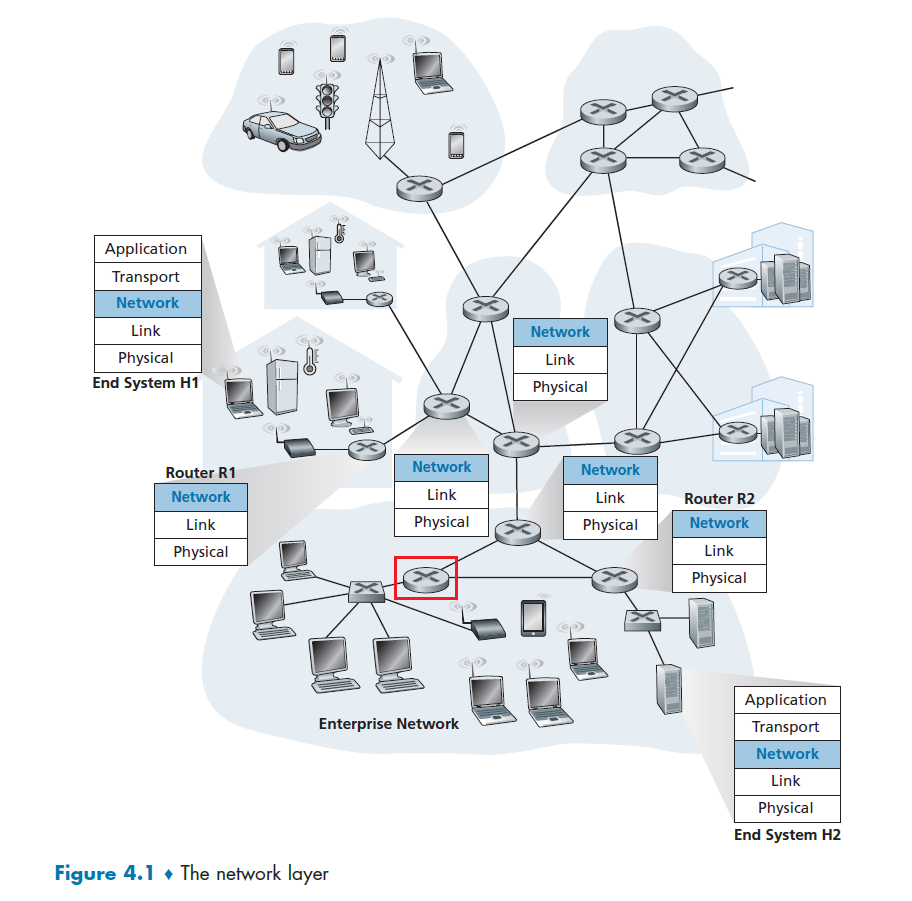
where:
- routers (the round ones) are in Network Layer (our focus)
- switches (the squared ones) are in Link Layer
The upshot is that basically a router/network layer has to do two things. Suppose you are at R1 and want to send stuff eventually to H2:
- Routing: you need to determine which next router to send to. (Routing Algorithm is in the control plane)
- Network-wide process. Takes place on much longer timescales (typically seconds), and as we will see is often implemented in software.
- Forwarding: once you determined which next hop is, move the packet to the appropriate output link (this is covered here)
- this sounds easy, but we need to do it as efficiently as possible
- Router-Local process. Forwarding takes place at very short timescales (typically a few nanoseconds), and thus is typically implemented in hardware
In particular, the data plane switches packet by using a key element in every network router is its forwarding table:
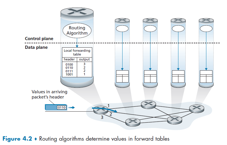
- examining the value of one or more fields in the arriving packet’s header (e.g. IP address)
- use the headers to index into the table and decide which router to send to
Quick Overview of Control Plane
Though it is not the focus here, it is good to know what it does on a high level.
Basically the routing algorithm needs to figure out the content of the forward table.
The traditional approach:
- A a routing algorithm runs in each and every router and both forwarding and routing functions are contained within a router. Routing algorithm function in one router communicates (via routing protocol) with the routing algorithm function in other routers to compute the values for its forwarding table
- so basically it is again a distributed algorithm that each router runs
- this has the advantage of you yourself can adjust your router’s algorithm to take into account some policies, such as minimize the cost of money
The modern Software-Defined Approach (SDN):
- A physically separate, remote controller computes and distributes the forwarding tables to be used by each and every router
- This is quite common in Data Centers: routing device performs forwarding only, while the remote controller computes and distributes forwarding tables.
- therefore, it is less flexible as it is a more localized setup, but it is more efficient if you are using it within your own network (e.g. the data center network)
- network is “software-defined” because the controller that computes forwarding tables and interacts with routers is implemented in software.
Graphically, the SDN looks like:
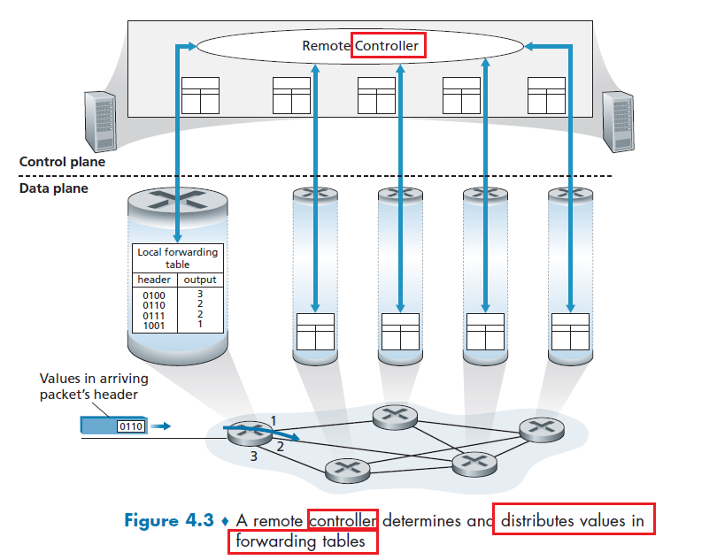
note that:
- the remote controller is not directly connected to each router. To send the forward tables to the router, we need routing itself to work to reach those routers from the controller. So if there is a failure, updates cannot be pushed to the router. This will basically becomes quite complicated.
- Again, the details will be covered in Chapter 5.
Overview of Services
Here we consider some potential services that a network layer can provide:
- Guaranteed delivery
- Guaranteed delivery with Bounded Delay
- In-order packet delivery
- Guaranteed Minimal Bandwidth
- Security
However, in reality, the Internet's network layer provides basically none of them:
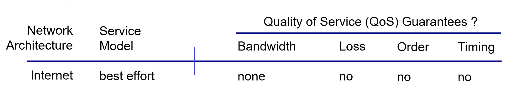
But it kind of works because
-
the Internet’s basic best-effort service model combined with adequate bandwidth provisioning and bandwidth-adaptive application-level protocols such as the DASH protocol we encountered in Section 2.6.2 have arguably proven to be more than “good enough” to enable an amazing range of applications. Also:
-
simplicity makes it widely adopted (hence easy to scale as well, e.g. CDNs)
Yet there are ofc algorithms that implements some of the service, but in reality the best effort one is the best
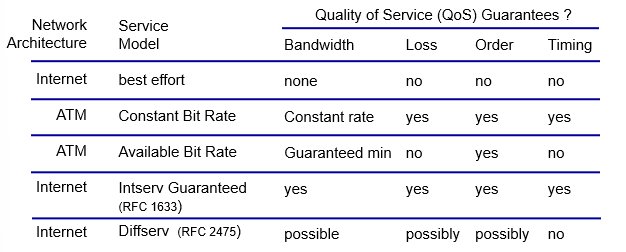
Inside A Router
let’s turn our attention to its forwarding function—the actual transfer of packets from a router’s incoming links to the appropriate outgoing links at that router.
First of all, a clarification of our previous abstraction:
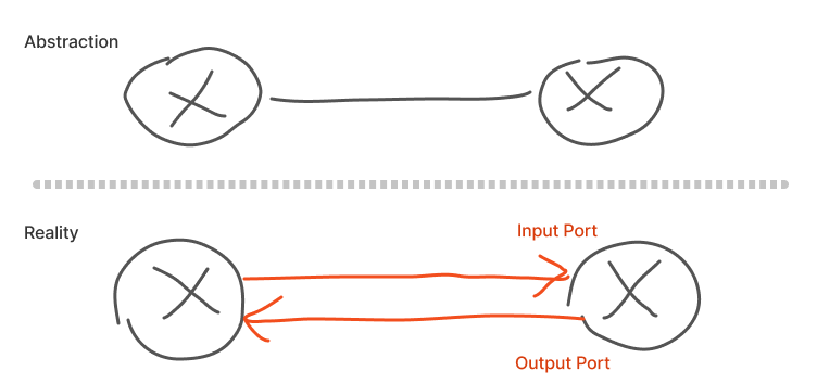
basically we don’t have bidirectional links in reality between two routers.
Now, it makes sense that a router has four components
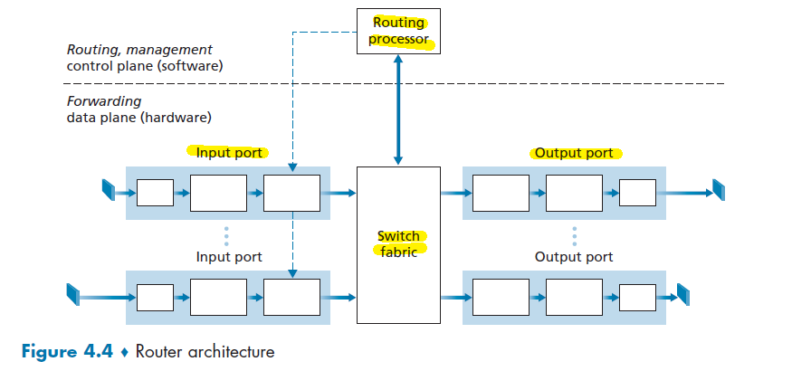
where here we assumed the router is connected to two routers, so we have two pairs of input/output port
- Switching fabric. The switching fabric connects the router’s input ports to its output ports. This must be fast so that we can fast fast internet
- Routing processor performs control-plane functions, e.g. by running routing algorithms and etc.
- basically this is for computing the look-up table. It will not interfere with the performance of switching in data plane.
- Input port and Output port will be covered below.
- notice that usually the forwarding plane here needs to operate as fast as possible! (much faster than control plane - routing algorithm)
Input Port Processing
A more detailed view of input processing is shown in Figure below.
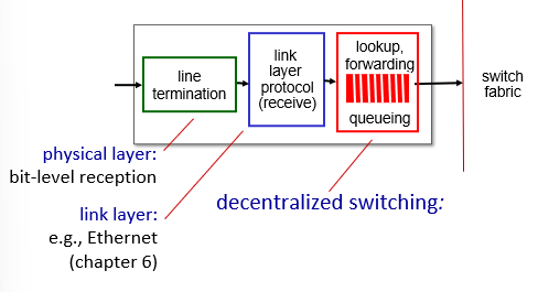
where basically the important part is the red part
-
input port’s line-termination function and link-layer processing implement the physical and link layers for that individual input link
-
lookup performed in the input port is central to the router’s operation—it is here that the router uses the forwarding table to look up the output port to which an arriving packet will be forwarded via the switching fabric
Let’s now consider the “simplest” case that the output port to which an incoming packet is to be switched is based on the packet’s destination address, i.e. the 32-bit IP. Then the table looks like:
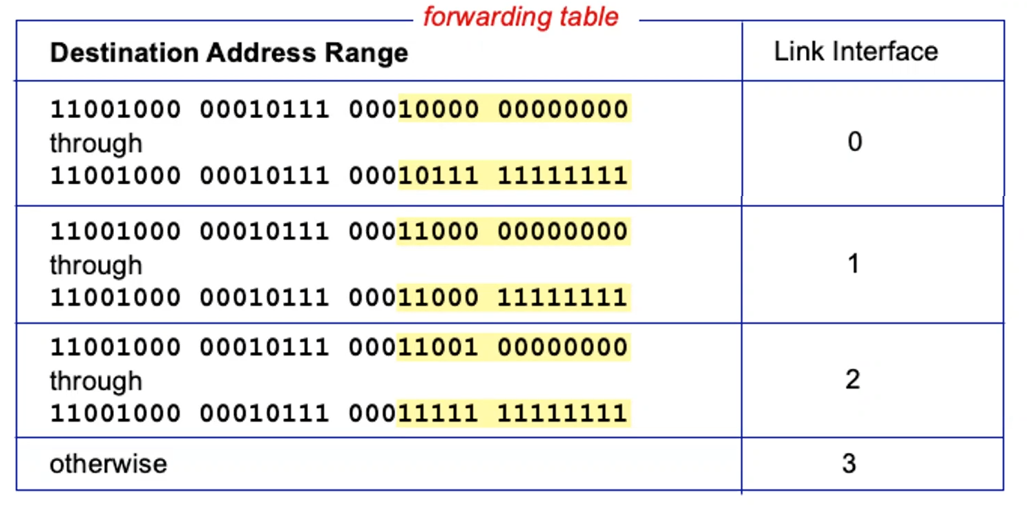
where note that:
- a brute force approach is to have an entry for each IP address, then there are $2^{32}$ options which is too large to store
- if you use a range, the problem is what if those ranges don’t divide up so nicely?
Note
- If you are on Columbia network, you will notice that all your devices’ IP has the form
160.39.xxx.xxx. In fact, those IP are distributed/granted for Columbian students to use are given in blocks: any $2^{16}$ addresses within160.39.0.0to160.39.255.255are allowed to use.- This also means that for some of the routers, all it matters is to determine where
160.39.xxx.xxxshould go! This is useful because:
- saves space in forwarding table, i.e. less entries
- routing decision can be made quicker only on those prefixes
Now, suppose the ranges don’t divide up so nicely, e.g. in a private network. Then:
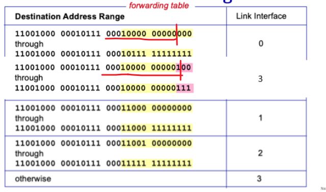
The router can perform a longest prefix match:
- e.g. if you have an IP of
1100xxxx xxxxxxx 00010000 00000101, then 3 will be returned as it has the longest match
Therefore, we see that router just need to store prefixes, and perform a longest prefix match. So routing table usually looks like this:
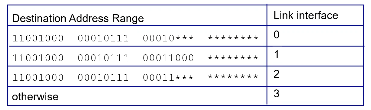
where notice that the length of prefix is variable, up to 32 bits.
Note that, at Gigabit transmission rates, this lookup must be performed in nanoseconds (e.g. for a 10 Gbps link and a 64-byte IP datagram, each packet needs to be sent within around 6 nanoseconds). Therefore, we need some fast hardware for memory access time
- this results in designs with embedded on-chip DRAM and faster SRAM (used as a DRAM cache) memories. In practice, Ternary Content Addressable Memories (TCAMs) are also often used for lookup.
- TCAM is expensive, but it can retrieve addresses in one clock cycle regardless of table size!
- i.e. when an IP address is given to TCAM, it gives you the link interface in one clock answer
Now, once you determine the output port/interface, you give it to switching fabric to do the actual switching
Note
- If packets from other input ports are currently using the fabric, a packet may be temporarily blocked from entering the fabric. A blocked packet will be queued at the input port and then scheduled to cross the fabric at a later point in time.
- Remember that although although “lookup” is arguably the most important action in input port processing, many other actions must be taken:
- physical- and link-layer processing must occur, as discussed previously;
- the packet’s version number, checksum and time-to-live field must be checked and the latter two fields rewritten;
- counters used for network management (such as the number of IP datagrams received) must be updated.
Switching Fabric
Once a packet’s output port/interface has been determined via the lookup, the packet can be sent into the switching fabric. In general, there three popular ways to do the switching:
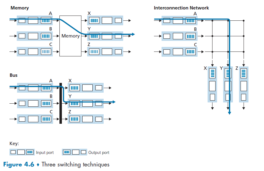
where
- we are interested in their switching rate: rate at which packets can be transferred from inputs to outputs
- often measured as multiple input/output line rate (i.e. when we have $N$ input/outputs)
- the slowest is memory, then bus, and finally now we use Interconnection Network.
Switching via Memory
The idea here is simple. Given a packet from a port, and we have a CPU (for the routing processor)
- write/copy the entire packet from input buffer into memory
- input port signaled the routing processor via an interrupt
- write/copy the packet from memory to the output buffer
- routing processor here does the lookup for the IP address and put it in the correct output buffer
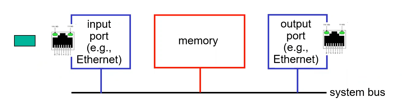
Therefore, for each single switching, we need to do 2 memory operations.
Switching via Bus
Basically a bus directly connects all input to all output. So the idea is that:
- Input does the lookup, and prepend the result as a header to the packet (switch -internal label)
- That packet is transferred to all output ports on the bus
- Each output bus checks the switch-internal label, and keeps the packet if there is a match
- i.e. only one output port will keep the packet in the end
- The matched output port removes the label, and you are done
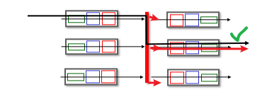
However, similar as above, if multiple packets arrive to the router at the same time, each at a different input port, all but one must wait since only one packet can cross the bus at a time.
Switching via Interconnection Network
Basically we want to be able to do simultaneous things, and the result is to consider the following:
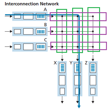
where if we have $N$ input/output ports, we take $2N$ bus, such that we have $N^2$ intersections. The idea is that each intersection can be opened or closed (packet can pass) at any time by the switch fabric controller (this part of logic is part of the switching fabric itself)
- e.g. if you send from $A$ to $Y$, then I just need to close the intersection of $A$ and $Y$ bus, and send to ALL bus! (but this time only $Y$ will receive it)
- therefore, if $A$-to-$Y$ and $B$-to-$X$ packets use different input and output busses, there is no blocking!
- but if you have $A-Y$ AND $B-Y$, then there is still blocking, i.e. one of them must wait.
Therefore, this could cause Head of Line blocking
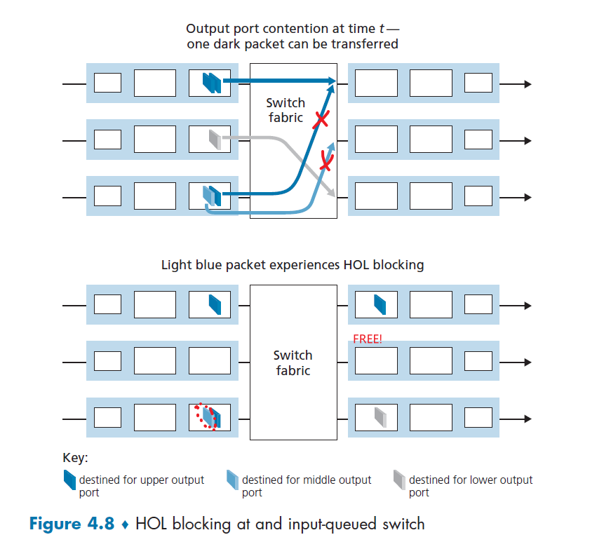
where basically:
- the first packet in the third input port has to WAIT, so the packet destined to the second output port is blocked
- the net result is one of the output port is FREE even if there is a message destined for the second output port (under utilization)
In fact, it is shown that due to HOL blocking, the input queue will grow to unbounded length (i.e. significant packet loss entails) if the packet arrival rate on input link reach
\[2-\sqrt{2} \approx 58 \% \text{ of capacity }\](basically you waste at least $42\%$ of the capacity)
To solve this issue, consider using virtual queue:
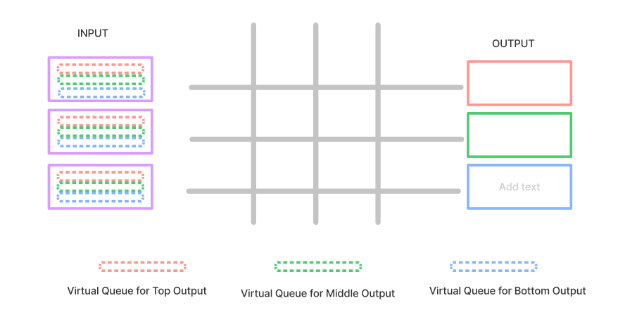
where now, no more HOL occurs and the for each clock cycle, you have 100% utilization.
- you still have queuing, but the utilization is now optimal
However, we CAN make packets from different input ports to proceed towards the same output port at the same time through the multi-stage switching fabric
Output Port Processing
Basically we know this already. Output port processing, essentially just need to take whatever that is passed to its output buffer, and transmit it.
- takes packets that have been stored in the output port’s memory
- transmits them over the output link.
- This includes selecting (i.e., scheduling) and de-queueing packets for transmission
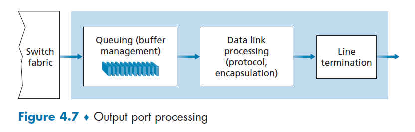
Queueing in Router
Note that queueing occurs at both Input port AND the output ports. Factors we need to consider here are:
- traffic load
- the relative speed of the switching fabric
- and the line speed
For instance, if each input port/output port (link) has a transmission rate of $R_{line}$ packets per second. If there are $N$ ports, then the worst case is you have $R_{line}\cdot N$ packets all going for the same output port.
- but if your switching fabric has $R_{switch}=R_{line}\cdot N$, then there is minimal INPUT queuing in the worst case all data is still placed on output ports. (But output port will have some queueing)
Input Port Queueing
Assume we are using crossbar, so multiple packets can be transferred in parallel, as long as their output ports are different. Then, we have:
- switch fabric $R_{switch} < R_{line}\cdot N$ is not fast enough to transfer all arriving packets through the fabric
- queuing occurs here regardless if data sent to the same output port or not
- Head of line blocking, causes queuing
Output Port Queueing
Now suppose the worst case again when all input ports are sending to the same output port, and assume each input/output port has a transmission rate of $R$ packets per second.
Then, for that output port:
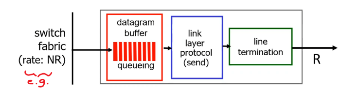
where basically:
- you get $NR$ messages coming in, but you can only transmit $R$ packets out
- so eventually queues build up at your output port, and if exceeds buffer/memory, packet is lost.
Since this is common and often unavoidable, we then need to consider:
- Drop Policy: if no free buffer left, which datagram/packet should we drop?
- Scheduling Discipline: which queued packet should be sent first for transmission, so that we ensure performance?
Buffer Length
Then the question is how much buffer is good for a port. Given the link capacity coming into/out of the router is $C$, and the average RTT is about $\text{RTT}$, then:
\[\text{buffer length} \approx \frac{\text{RTT}\cdot C}{\sqrt{N}}\]for $N$ being the number of input/output ports.
- notice that this comes from the fact that “more buffering might not be better” as buffering can be used to absorb short-term statistical fluctuations in traffic but can also lead to increased queuing delay. (large buffers means larger queueing delay, which might even be worse than dropping packets if you are gaming)
- basically this is to make sure your queuing delay is not too large
For Example:
Consider the setup of a gamer’s house with a router being able to send a packet every $20 ms$. Suppose the RTT to the gaming server is $200ms$, and suppose there is no other queuing delay on the network except for the home router. Then:
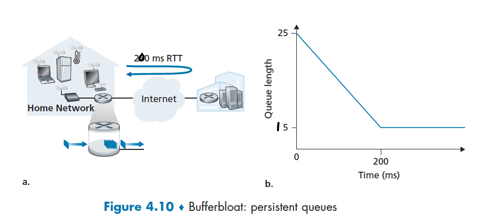
- suppose at $t=0$, router got 25 packets in a burst
- after $t=200ms$, the first ACK comes back, but we only sent $10$ packets
- the next TCP packet is now sent, but it has to wait for 15 packets in front! Resulting in some queueing delay due to the buffer size being large.
This scenario is also called the Buffer Bloat.
Packet Scheduling
Basically we need to consider the problem of determining the order which packets are transmitted. (Also related to which packets to drop)
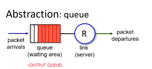
Some basic ideas are:
- FCFS
- Priority Queuing
- Round Robin
- Weighted Fair Queue
Scheduling: FIFO
Basically, assume that each packet takes three units of time to be transmitted. Under the FIFO discipline, packets leave in the same order in which they arrived.
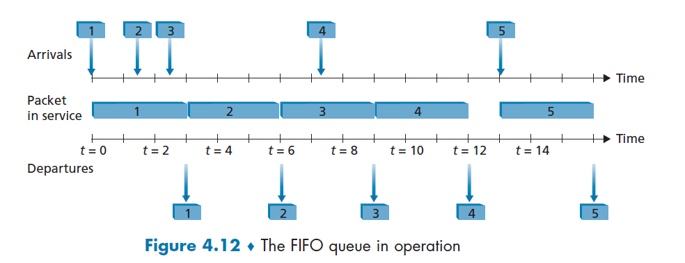
Scheduling: Priority
Now, sometimes real time application such as Voice communication needs to be transmitted with low latency. In this case, consider splitting packets into different priority (e.g. by looking at which port it comes from).
Then, the idea is to transmit a packet from the highest priority class that has a nonempty queue (i.e. low priority only looked at when high priority are all gone - i.e. could be exhausted).
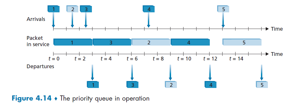
where in this example:
- Packets 1, 3, and 4 belong to the high-priority class
- packets 2 and 5 belong to the low-priority class
Scheduling: RR
Basically, the only difference here is that:
- you still have multiple classes
- RR transmit one packet per class, and moves on next
Therefore, assuming we have two classes (e.g. could be priority class):
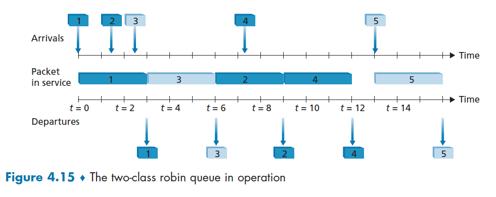
where again:
- packets 1, 2, and 4 belong to class 1, and packets 3 and 5 belong to the second class
- packet 3 is transmitted before packet 2 because RR checks the next class to be fair
Scheduling: WFQ
The principle is basically just a Weighted Round Robin, where you assign a weight $w_i$ to each class representing how important they are, so that class i will then be guaranteed to receive a fraction of service equal to:
\[\frac{w_i}{\sum_i w_i} \text{ of the service time}\]Therefore, basically it circulates through all the classes but gives more time on more important classes.
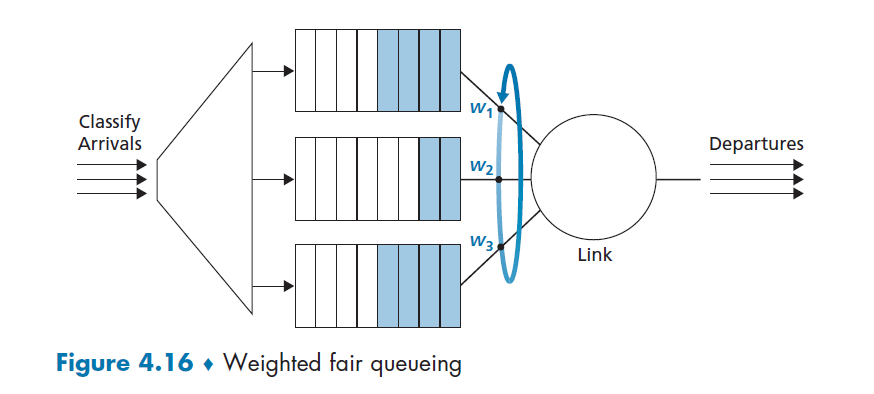
This is also implemented the most today.
Network Neutrality
The idea of giving weight/class for different classes gives ISP/providers for routers some choices to exploit it:
- prioritize packets from specific IP (e.g. business that paid more)
- charge packets from specific IP more than others (e.g. charge packets from Google less)
- etc
Those basically gives unfair advantages for some content providers, which is bad, so there are laws that goes against them.
The IP Protocol: IPv4, IPv6 and more
A roadmap of where we are:
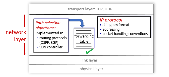
basically we have discussed how forwarding table works, and now we look at the content of packet in IP protocol.
IPv4 Datagram Format
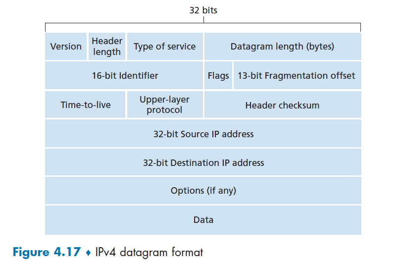
where basically:
- Version number. These 4 bits specify the IP protocol version of the datagram
- Header length. Because an IPv4 datagram can contain a variable number of options
- Type of service. The type of service (TOS) bits were included in the IPv4 header to allow different types of IP datagrams.
- e.g. distinguish real time datagrams from non-real-time traffic
- e.g. the last two TOS bits are used for Explicit Congestion Notification, ECN.
- Datagram length. This is the total length of the IP datagram (header plus data), measured in bytes.
- Since it is 16 bit, the theoretical maximum size is 65,535 bytes. However, datagrams are rarely larger than 1,500 bytes, which allows an IP datagram to fit in the payload field of a maximally sized Ethernet frame
- Identifier, flags, fragmentation offset. These three fields have to do with so-called IP fragmentation. Basically used when reassembling the packet
- .e. configured when it is fragmented, used when reassembling
- Time-to-live. The time-to-live (TTL) field is included to ensure that datagrams do not circulate forever. This is decremented by 1 every time when a router processed the packet
- Protocol. This field is typically used only when an IP datagram reaches its final destination. The value of this field indicates the specific transport-layer protocol its data field has, e.g. TCP or UDP.
- Header checksum. The header checksum aids a router in detecting bit errors in a received IP datagram
- notice it is only for the IP headers, not for payload
- Source and destination IP addresses. When a source creates a datagram, it inserts its IP address into the source IP address field and inserts the address of the ultimate destination into the destination IP address field
- Options: allow an IP header to be extended. Header options were meant to be used rarely.
- Data/Payload: data field of the IP datagram contains the transport-layer segment (TCP or UDP) to be delivered to the destination
IPv4 Addressing
First of all, a few terminologies:
-
(Network) Interface: the boundary between the host and the “physical” link is called an interface.
- e.g. your laptop has two interface, one for Ethernet link, one for Wireless link
- e.g. a router with $N$ input port has $2N$ interfaces.
-
dotted-decimal notation that IP uses:
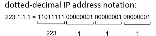
where router basically use the binary form only (e.g. lookup table)
-
Subnet: A network that contains connected hosts but with no routers, so hosts talk to each other directly
- for example, the top left network in Figure 4.18 is a subnet, with
233.1.1.0/24
- for example, the top left network in Figure 4.18 is a subnet, with
Then, the setup is:
- IP address is technically associated with an interface (one end of a connection), not with a host
- e.g. if you have 2 interfaces, you have 2 IP
- IP address is not given randomly, a portion of an interface’s IP address will be determined by the subnet
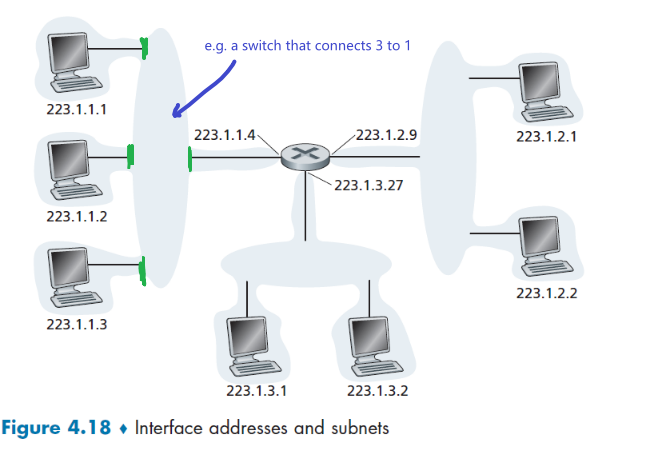
where notice that:
- if the top left subnet is defined by
233.1.1.0/24, it means the first 24 bit is a subnet mask, that the first 24 bits is shared for interfaces in that network. i.e. all must have the IP of223.1.1.xxx - An organization is typically assigned a block of contiguous addresses, that is, a range of addresses with a common prefix
Classless Interdomain Routing (CIDR)
- basically instead of forcing a choice of either 8,16,24 bits for mask, you can now have something like 21 bits for mask. This is so that you can have:
a.b.c.d/21being the organization’s blocka.b.c.d/24a specific subnet within the organization
So the subnet structure of the Figure 4.18 is basically:
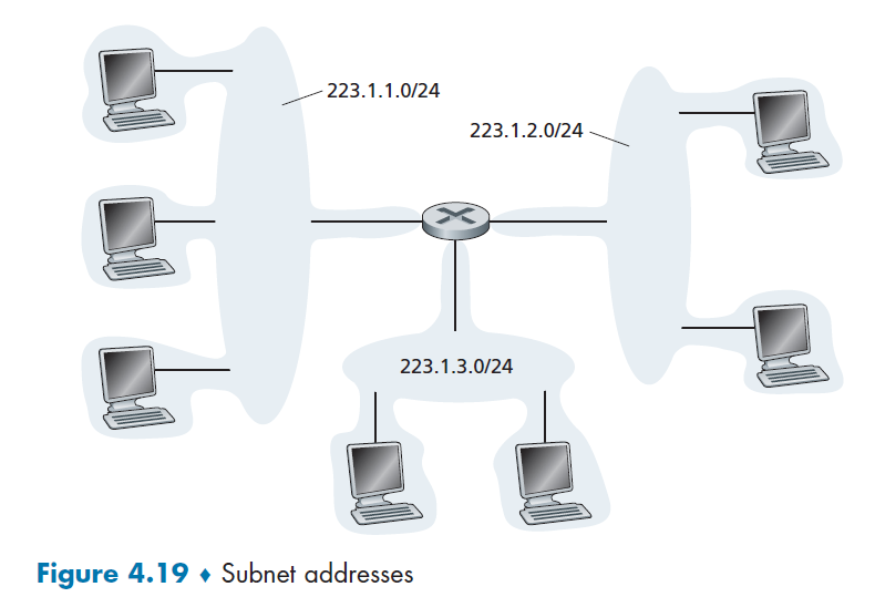
A more complicated example would be:
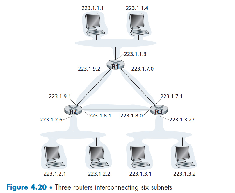
where now you have 6 subnets.
Now, we know how the IP address means. The question is how is it assigned?
- how does Host get an IP within a subnet?
- how does the entire network know which IP range to use?
Obtaining Host Address: DHCP
Before, those IP address are configured by hand by the network administrator. Now they are automated using DCHP.
DHCP allows a host to obtain (be allocated) an IP address automatically.
- in fact, it’s a server that also tells your device its subnet mask, the address of its first-hop router (often called the default gateway, which is different from gateway router), and the address of its local DNS server
- the IP of gateway router may sound “useless” at this point, but you will see in Routing to Another Subnet that this will be used for figuring our the MAC address of that router (using ARP broadcast), and then getting the packet to the router which connects to the outer world (via Link Layer delivering packets through those switchess)
DHCP’s advantage is that/works because:
-
people tend to spend only limited amount of time using the internet anyway, so permanent IP address is wasteful (since there is only a limited amount of IP addresses)
-
each person’s IP is not important, i.e. we are not well known serves that people need to know our IP beforehand!
DHCP is a client-server protocol.
- A client is typically a newly arriving host wanting to obtain network configuration information, including an IP address for itself.
- In the simplest case, each subnet (in the addressing sense of Figure 4.20) will have a DHCP server. In some other times a router of a subnet can act as a relay to another DCHP server.
Therefore, when your laptop is connected to a subnet:
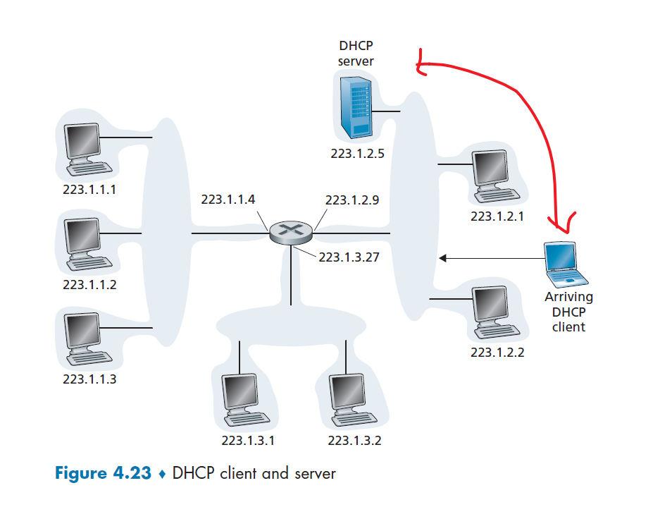
Detailed steps of what happened is shown here:
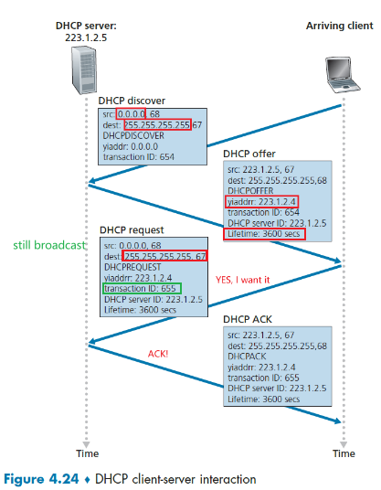
- DHCP server discovery. The first task of a newly arriving host is to find a DHCP server with which to interact. This is done using a DHCP discover message. This is done by a client send a UDP packet to port
67.- but who to send it to? The client has no idea what IP is even used. This is basically done by a broadcasting message with
dest=255.255.255.255andsource=0.0.0.0
- but who to send it to? The client has no idea what IP is even used. This is basically done by a broadcasting message with
- DHCP server offer(s). A DHCP server receiving a DHCP discover message responds to the client with a DHCP offer message that is broadcast to all (because the client now has no IP)
- therefore,
dest=255.255.255.255:68where port68is where sender initiated the request - some important fields here include
your_ip_address=yiaddrwhich is the offer, and the lifetime (after which you need to refresh)
- therefore,
- DHCP request. The newly arriving client will choose from among one or more server offers and respond to its selected offer with a DHCP request message, echoing back the configuration parameters.
- notice it is another broadcast since it needs to tell all DCHP servers.
- also notice that
DCHP Discoverhas a different transaction ID thanDCHP Request
- DHCP ACK. The server responds to the DHCP request message with a DHCP ACK message, confirming the requested parameters.
- this is when you are finally done.
Broadcast IP address
- the IP broadcast address
255.255.255.255. When a host sends a datagram with destination address255.255.255.255, the message is delivered to all hosts on the same subnet. Routers optionally forward the message into neighboring subnets as well (although they usually don’t).
Obtaining Network Address: Address Aggregation
The Internet’s address assignment strategy is known as Classless Interdomain Routing (CIDR—pronounced cider), which we covered before. Here, we provide an example of ISP that connects eight organizations to the Internet, to show how carefully allocated CIDRized addresses facilitate routing.
-
the ISP (which we’ll call Fly-By-Night-ISP) advertises to the outside world that it should be sent any datagrams whose first 20 address bits match
200.23.16.0/20. The rest of the world need not know that within the address block200.23.16.0/20there are in fact eight other organizations, each with its own subnets.- This ability to use a single prefix to advertise multiple networks is often referred to as address aggregation (also route aggregation or route summarization).
-
Organization 1 now switched the ISP to ISPs-R-Us
Then either you need to:
- Organization 1 could renumber all of its routers and hosts to have addresses within the ISPs-R-Us address block
199.31.0.0/16. (costly if we need to do this everytime when switched to a new ISP) - Organization 1 to keep its IP addresses in
200.23.18.0/23, and the ISP do something (right figure)
- Organization 1 could renumber all of its routers and hosts to have addresses within the ISPs-R-Us address block
-
The solution commonly employed is to let Organization 1 keep its IP addresses, but ISPs-R-US also advertises
200.23.18.0/23, which would work due to longest prefix matching. (data sent to organization 1 matches both ISP, but the longest prefixing matching means they will be forwarded to ISPs-R-US.)- note that you might want to do some merging of addresses afterwards in ISPs-R-Us if this happens often
| Router Aggregation | ISPs-R-Us has a more specific route |
|---|---|
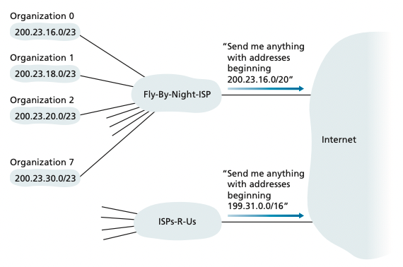 |
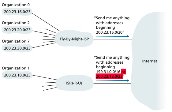 |
Network Address Translation: NAT
Basically it is a trick to saving IP addresses:
-
there are three portions of IP address space that is reserved in [RFC 1918] for a private network or a realm with private addresses:
192.168.0.0–192.168.255.255172.16.0.0–172.31.255.25510.0.0.0–10.255.255.255
Then, this means that they are thousands of devices have the same IP in those range, but the meaning of their IP only makes sense within their network.
- Devices within a given home network can send packets to each other using those IP only within the network.
-
NAT-enabled router does not look like a router to the outside world. Instead the NAT router behaves to the outside world as a single device with a single IP address.
Graphically:
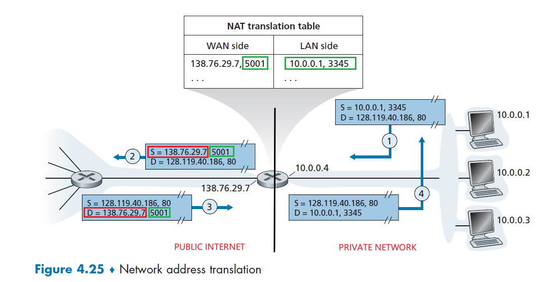
where we see that:
- all traffic leaving the home router for the larger Internet has a source IP address of
138.76.29.7, and all traffic entering the home router must have a destination address of138.76.29.7. - use a NAT translation table to know finally which device to forward to by essentially port $\to$ IP + port
Note then this basically means we are using one IP for all your private devices! (hence essentially saving some IP addresses for use)
Now, in this case, the IPs are configured by:
- the router gets its address from the ISP’s DHCP server,
- the router runs a DHCP server to provide addresses to computers within the NAT-DHCP-router-controlled home network
However, some problems you need to consider:
- routers should only process up to layer 3, this is doing too much customization
- NAT traversal: what if client wants to connect to a server behind NAT? Need more configuration.
- technically you can hard-code the mapping, but in the end it requires quite a lot of work.
Obtaining Block of Address
Now, how does Columbia for example get the 160.39.0.0/16 block? Basically:
- given by the upstream ISP
- (the upstream ISP eventually gets their IPs from ICANN, which is Internet Corporation for Assigned Names and Numbers)
For example
The ISP may itself have been allocated the address block 200.23.16.0/20. The ISP, in turn, could divide its address block into subspaces and give to organizations:
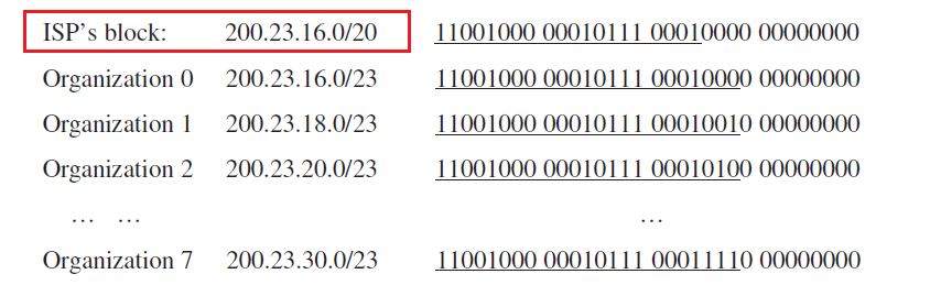
IPv6
Basically used for the problem of IPv4 running out of addresses. This has the advantage of:
- more IP address available, now it is $2^6=128$ bits
- fixed 40-byte length header, so faster processing speed
Then the datagram format looks like:
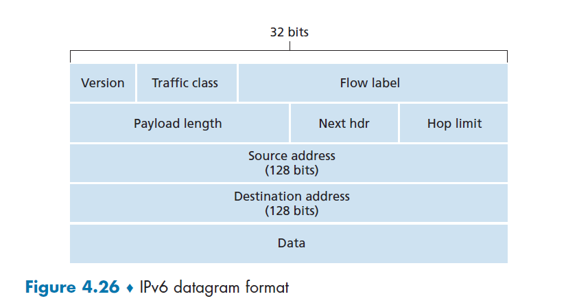
where:
- Version. This 4-bit field identifies the IP version number. Not surprisingly, IPv6 carries a value of
6in this field - Traffic class. The 8-bit traffic class field, like the TOS field in IPv4, can be used to give priority to certain datagrams within a flow
- Flow label. As discussed above, this 20-bit field is used to identify a flow of datagrams (meaning of flow still not well defined today)
- Payload length. This 16-bit value is treated as an unsigned integer giving the number of bytes in the IPv6 datagram following the fixed 40 byte header.
- Next header. This field identifies the protocol to which the contents (data field) of this datagram will be delivered (for example, to TCP or UDP)
- Hop limit: TTL
- Source and destination addresses. The various formats of the IPv6 128-bit address
- Data: same as the data in IPv4 packet, basically the TCP/UDP segment.
What is missing here is:
- Fragmentation/reassembly. IPv6 does not allow for fragmentation and reassembly at intermediate routers
- Header checksum. Because the transport-layer (for example, TCP and UDP) and link-layer (for example, Ethernet) protocols in the Internet layers perform check-summing, the designers of IP probably felt that this functionality was sufficiently redundant.
- Options: just as TCP or UDP protocol headers can be the next header within an IP packet, so too can an options field
Tunning from IPv4 to IPv6
Many routers are now using IPv4, if you send IPv6, how does that work?
Heuristics
IPv6 datagram carried as payload in IPv4 datagram among only IPv4 enabled routers.
As a result, those packets look like:
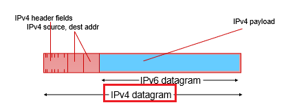
Then, what you do is:
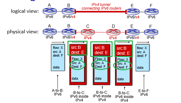
where:
- for IPv6 enabled routers, they transmit the message normally
- the receiver IPv6 (node E) will realize that the datagram has
protocol=41in the header, which means IPv6 embedded in payload.
- the receiver IPv6 (node E) will realize that the datagram has
- for IPv4 router, in the tunnel route this IPv4 datagram among themselves, just as they would any other datagram
- note that the
source/dest IPin the packets become the 32-bit IP of router `B,E` respectively. This makes sense since now the IPv6 IP is 128 bits.
- note that the
Generalized Forwarding and SDN
Basically this is the extension of the idea that match-plus-action used for sending packet from input port to output port can be used in many other functionalities such as load-balancing, firewalling, etc. Essentially, instead of considering matching a single header/doing a single action:
- match a set of headers and perform a set of actions
- have each router store a table of match-plus-action table (local flow table)
Note
- since now we could match headers potentially using link-layer headers, this is more general than a router. Hence, those routers are often referred to as packet switches (different form both a router and linl-layer switch)
- hence we will refer to those routers are packet switches for this section
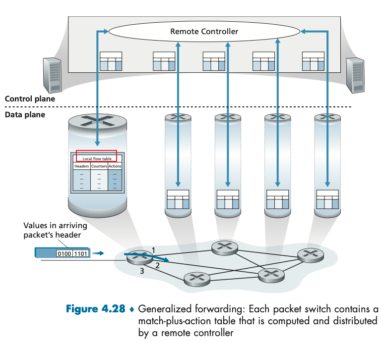
note that
- while it is possible for the control components at the individual packet switches to interact with each other (e.g., in a distributed manner similar to that in Figure 4.2), in practice, generalized match-plus-action capabilities are implemented via a remote controller that computes, installs, and updates these flow tables.
- essentially the flow table is a programmable API such that we can control the behavior of individual packet switch
- Figure 4.28 is an example of the OpenFlow 1.0 architecture, where the flow table eseentially includes:
- a set of header field values to which an incoming packet will be matched.
- a set of counters that are updated as packets are matched to flow table entries. These counters might include the number of packets that have been matched by that table entry, and the time since the table entry was last updated.
- a set of actions to be taken when a packet matches a flow table entry. These actions might be to forward the packet to a given output port, to drop the packet, makes copies of the packet and sent them to multiple output ports, and/or to rewrite selected header fields.
Chapter 5 Network Layer: Control Plane
In the data plane, we had forwarding table (in the case of destination-based forwarding) and the flow table (in the case of generalized forwarding) were the principal elements that linked the network layer’s data and control planes.
Then, in this chapter, we learn how those forwarding and flow tables are computed, maintained and installed.
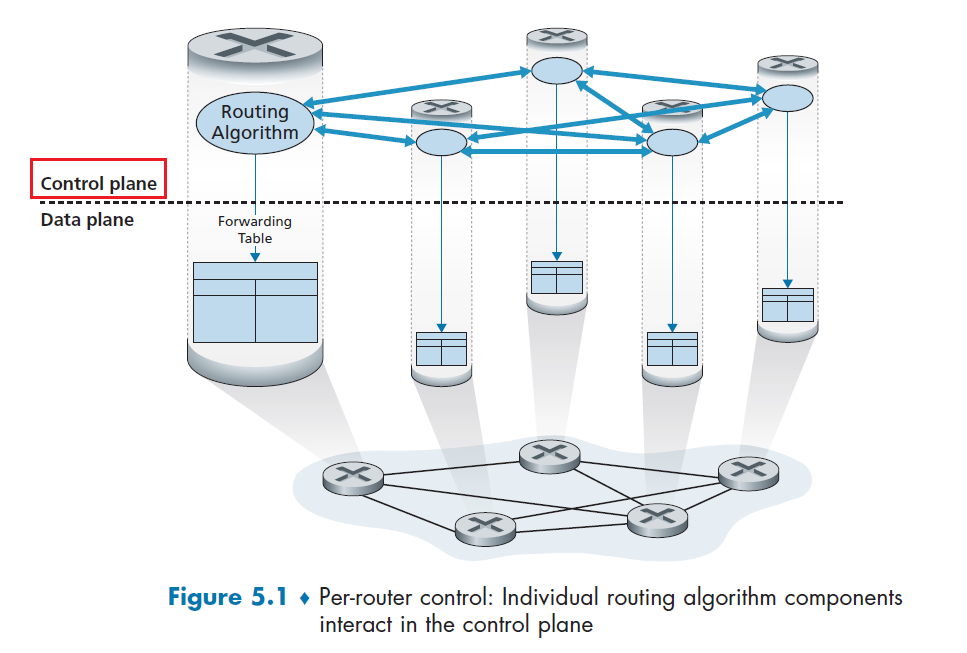
where:
- Each router has a routing component that communicates with the routing components in other routers to compute the values for its forwarding table
- while the routing algorithm runs, the data plane stuff runs in parallel
Additionally, we basically want to make routing scalable. So we also need the hierarchy design principles:
- the basic idea is to split the work to: a) route within a network, b) route between networks (autonomous system)
- i.e. for Google to reach your device at Columbia, Google just needs to know how to route to Columbia. Then, the Columbia network/gateway routers will route to your device
Logically Centralized Control
As we have discussed above, we could have also centralized everything
where here we:
- lose the scalability
- The controller interacts with a control agent (CA) in each of the routers via a well-defined protocol to configure and manage that router’s flow table
- CA has minimum functionality; its job is to communicate with the controller, and to do as the controller command
- unlike the other case, here CAs do not directly interact with each other
Routing Algorithms
Now we study routing algorithms, whose goal is to determine good paths (equivalently, routes), from senders to receivers, through the network of routers.
- Typically, a “good” path is one that has the least cost. We’ll see that in practice, however, real-world concerns such as policy issues, so cost is defined differently at different places.
- no matter you use the per-router approach or the logically centralized approach, we always need a well-defined sequence of routers for the path
Here, we first formalize our discussion with graphs:
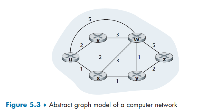
where we have $G=(N,E)$ being the set of nodes and weighted edges
- it is an undirected graph
- weight represent cost, e.g. $c(x,y)=1$ could be cost of delay, monetary cost, or etc
So our goal in this chapter is to find a least-cost paths between sources and destinations.
- if cost are the same, then least-cost path = shortest path
Now, in reality, we actually use per-router algorithm (decentralized) and locally centralized algorithm (centralized) together. Therefore, we consider:
- centralized routing algorithm:
- The algorithm knows connectivity between all nodes and all link costs as inputs in advance. Then, since it knows the complete information, it can just perform a Dijkstra algorithm.
- Algorithms with global state information are often referred to as link-state (LS) algorithm.
- decentralized routing algorithm:
- No node has complete information about the costs of all network links. Each node only has info about its immediate neighbors. So we will need some iterative process of calculation and exchange of information with its neighboring nodes to compute a least cost
- here we use distance-vector (DV) algorithm, because each node maintains a vector of estimates of the costs (distances) to all other nodes
Other Algorithm Classes
Some other classification of algorithms include:
- static vs dynamic routing algorithms: whether if route changes in direct response of chance of topology
- load-sensitive vs insensitive algorithms: whether if link costs vary dynamically to reflect the current level of congestion in the underlying link
Link-State Routing Algorithm
Recall that in a link-state algorithm, the network topology and all link costs are known in advance.
- To deliver all the info in advance, we need each node broadcast link-state packets to all other nodes in the network, with each link-state packet containing the identities and costs of its attached links. (this is done in practice by the link-state broadcast algorithm)
- The result of the nodes’ broadcast is that all nodes have an identical and complete view of the network. Then, each node can just run the LS algorithm (Dijkstra’s Algorithm)
Dijkstra’s algorithm computes the least-cost path from one node (the source, which we will refer to as $u$) to all other nodes in the network.
- $D(v)$: cost/distance of the least-cost path from the source node to destination $v$ as of this iteration of the algorithm.
- $p(v)$: previous node (neighbor of $v$) along the current least-cost path from the source to $v$.
- $N’$: subset of nodes; $v$ is in $N’$ if the least-cost path from the source to $v$ is definitively known. (i.e. is done)
Then the Dijkstra Algorithm is doing:
-
initialization
-
perform the Greedy Step, assuming the one with smallest $D$ is already settled/known (put in $N’$)
Vertex Known Dv/Distance Pv/Previous $V_1$ T 0 N/A $V_2$ F $\infty$ $V_1$ $V_3$ F $\infty$ - $V_4$ F $\infty$ $V_1$ $V_5$ F $\infty$ - $V_6$ F $\infty$ - $V_7$ F $\infty$ - -
run through the Adjacency List/Neighbor of that settled vertex and update the table
- try to add the value of $D$ of the settled vertex up to each of the vertex in the list
- we update the $D$ only when it is better than the current $D$ belonging to that vertex
Vertex Known Dv/Distance Pv/Previous $V_1$ T 0 N/A $V_2$ F 2 $V_1$ $V_3$ F $\infty$ - $V_4$ F 1 $V_1$ $V_5$ F $\infty$ - $V_6$ F $\infty$ - $V_7$ F $\infty$ - -
Repeat step 3 to 4 until all vertices are known
e.g. the next iteration of step 2 becomes:
Vertex Known Dv/Distance Pv/Previous $V_1$ T 0 N/A $V_2$ F 2 $V_1$ $V_3$ F $\infty$ - $V_4$ T 1 $V_1$ $V_5$ F $\infty$ - $V_6$ F $\infty$ - $V_7$ F $\infty$ - so eventually a path from $V_1$ to any other node is recorded by $P$.
In terms of code, it looks like:
// again, we assumes a non-negative cycle

void dijkstra(Vertex s){
    for each Vertex v{
        v.dist = INFINITY;
        v.known = false;
    }

    s.dist = 0;

    // this happens |V| times
    while(there is an unknown vertex){
        // if you find the min by scanning through the list
        // then this is also |V|
        Vertex v = smallest known vertex

        v.known = true;

        // this loop goes IN TOTAL |E| times
        for each Vertex w adjacent to v{
            if(!w.known){
                // the next step/edge's cost
                DistType cvn = cost of edge from v to w;

                // if we did find something smaller
                if(v.dist + cvn < w.dist){
                    // update w
                    // in this version, w.dist = v.dist+cvw works the same

                    // this is useful, because there is actually ANOTHER way of doing this
                    decrease(w.dist to v.dist+cvn);
                    w.pv = v;
                }
            }
        }
    }
}
Therefore, this algorithm tells us that when the LS algorithm terminates, we have, for each node, its predecessor along the least-cost path from the source node.
Then the forwarding table in node $u$ will basically be the next-hop node on the shortest path to $t$:
| Graph | Forwarding Table for $u$ |
|---|---|
|
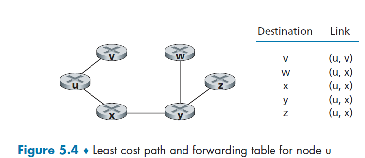 |
(note that the worst case computation complexity for this is $O(N^2)$)
Oscillations of Dijkstra’s Algorithm
When link cost depends on traffic volume, route oscillation is possible, because the cost itself then changes based on whether if I chose a specific route or not.
For instance, consider sending stuff from C to A. Let B want to same traffic of 1, C want to send traffic of e, and D want to send traffic size of 1, Then:
| t=0 | t=1 | t=2 | t=3 |
|---|---|---|---|
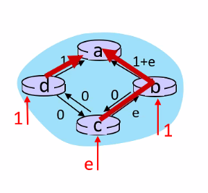 |
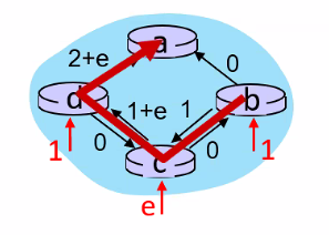 |
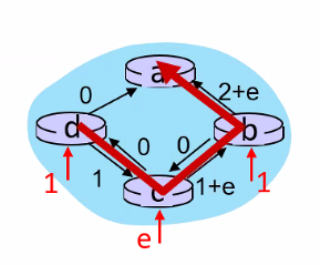 |
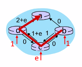 |
least weightC-B-A |
least weight C-D-A |
least weightC-B-A |
least weight C-D-A |
where basically:
- suppose at
t=0we have the route computed already to beC-B-A. Since we are sending stuff which will cause an increase in traffic, this causes the same route to have a cost of $e+(1+e)$ - then, since the other route
C-D-Ahas only a cost of $1$, we switch toC-D-A. But now we are sending traffic there as well! So at $t=1$ we know have a cost of $e+(1+e)$, - repeat
- notice that $t=0=2$ and $t=1=3$ happens because each router updates the new path at the SAME TIME
Solution
- mandate that link costs not depend on the amount of traffic [not acceptable]
- doesn’t make sense since the aim of routing is to avoid congestion = high traffic!
- ensure that not all routers run the LS algorithm at the same time
- e.g. randomize the time it sends out a link advertisement.
Distance-Vector Routing Algorithm
This basically is an iterative and distributive algorithm, because:
- distributive: each node receives some information from one or more of its directly attached neighbors, performs a calculation, and then distributes the results of its calculation back to its neighbors.
- iterative: this process continues on until no more information is exchanged between neighbors
First thing to notice is that, for the Greedy Algorithm to work, we neede the Bellman-Ford Equation that, if $d_X(y)$ is the cost of least-cost path from $x$ to $y$, then:
\[d_x(y) = \min_v \{ c(x,v) + d_v(y) \}\]which makes sense as $d_v(y)$ is the min path, and we have positive edges only.
- after traveling from $x$ to $v$, if we then take the least-cost path from $v$ to $y$, the path cost will be $c(x, v) + d_v(y)$.
- therefore, if $v^*$ is the neighbor of $x$ and achieves the $\min$, then the forwarding table to get data from $x\to y$ means $x$ should forward to $v^*$.
- this is technically the same equation used in Dijkstra’s algorithm
Graphically, it is just doing:
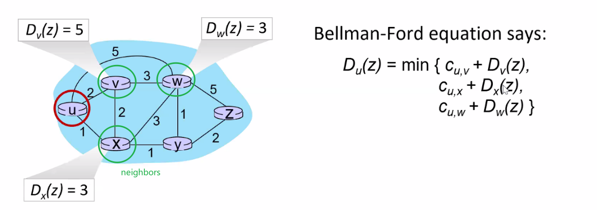
where:
- the best path from $D_u(z)$ would be $\min(\text{path to neighbor} + \text{path from neighbor to$z$})$
- therefore, this basically is done iteratively for all nodes until no changes/all information propagated
Then the algorithm is as follows:
Initialization:
	for all destinations y in Node:
		Dx(y)= c(x,y) /* if y is not a neighbor then c(x,y)= infty */
	for each neighbor w
		Dw(y) = ? for all destinations y in N
	for each neighbor w
		send distance vector Dx = [Dx(y): y in N] to w

Main loop
	wait (until I see a link cost change to some neighbor w or
		until I receive a distance vector from some neighbor w)

	for each y in N:
		Dx(y) = min_v{c(x,v) + Dv(y)} /* Bellman-Ford Equation, update distance vector */

	if Dx(y) changed for any destination y /* tell others IFF there is a change! */
		send distance vector Dx = [Dx(y): y in N] to all neighbors

forever
basically the key idea is that, for a node $x$ in the graph:
-
initialize all cost $D_x(y)$ to any other node in the graph ($D_x(y)=c(x,y)$ if $y$ is a neighbor, otherwise initialize with $\infty$)
-
send your current $D_x(y)$ vector to your neighbor
-
receive $D_v(y)$ from your neighbor $v$, and update your $D_x(y)$ since you can now compute:
\[D_x(y) \leftarrow \min_v \{ D_v(y) + c(x,v) \}\]where $c(x,v)$ you can directly measure by $x$ itself since $v$ are its neighbor
-
send the $D_x(y)$ result that changed to your neighbors (so they can update)
-
repeat 2-4 until no changes
For Example
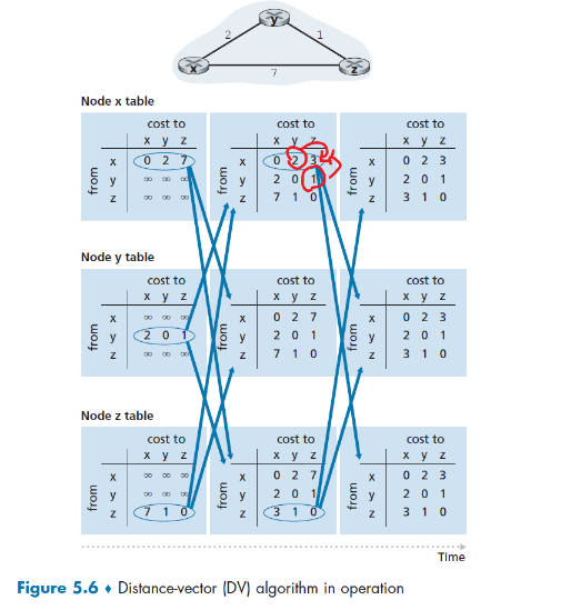
where notice that:
- each row is a distance vector in the algorithm
- the update on the
xtable for $x-y$ in iteration 2 happens because $c(x,y)+D_y(z)=3$ is smaller than the current value $7$. Therefore, we have updated the table - remember that in the end we just need to know the next-hop for the table! So we also needed store the next hop information as well when updating our $D_x(y)$.
Another more animated view is this (here we only focus on router b)
| t=1 | t=2 |
|---|---|
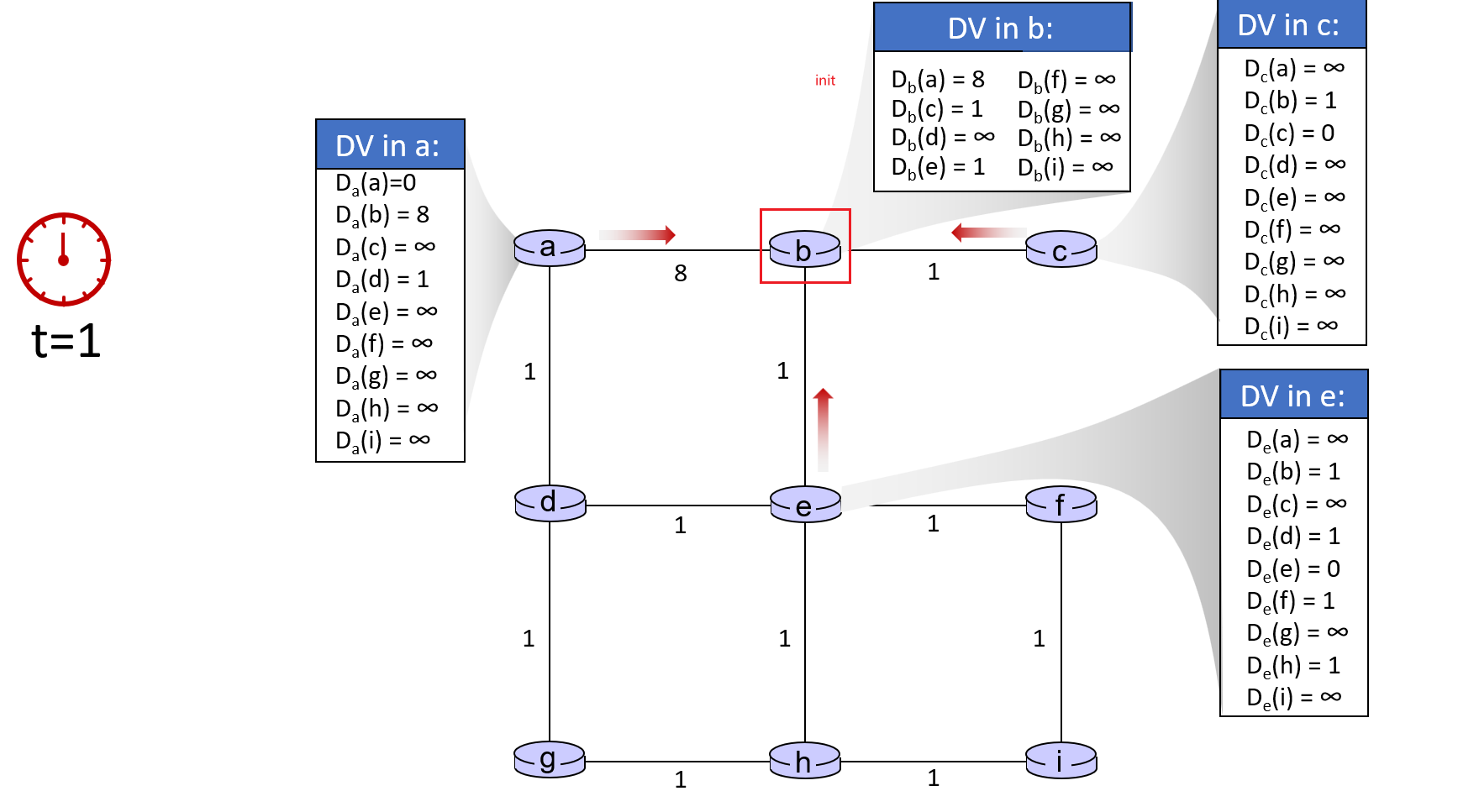 |
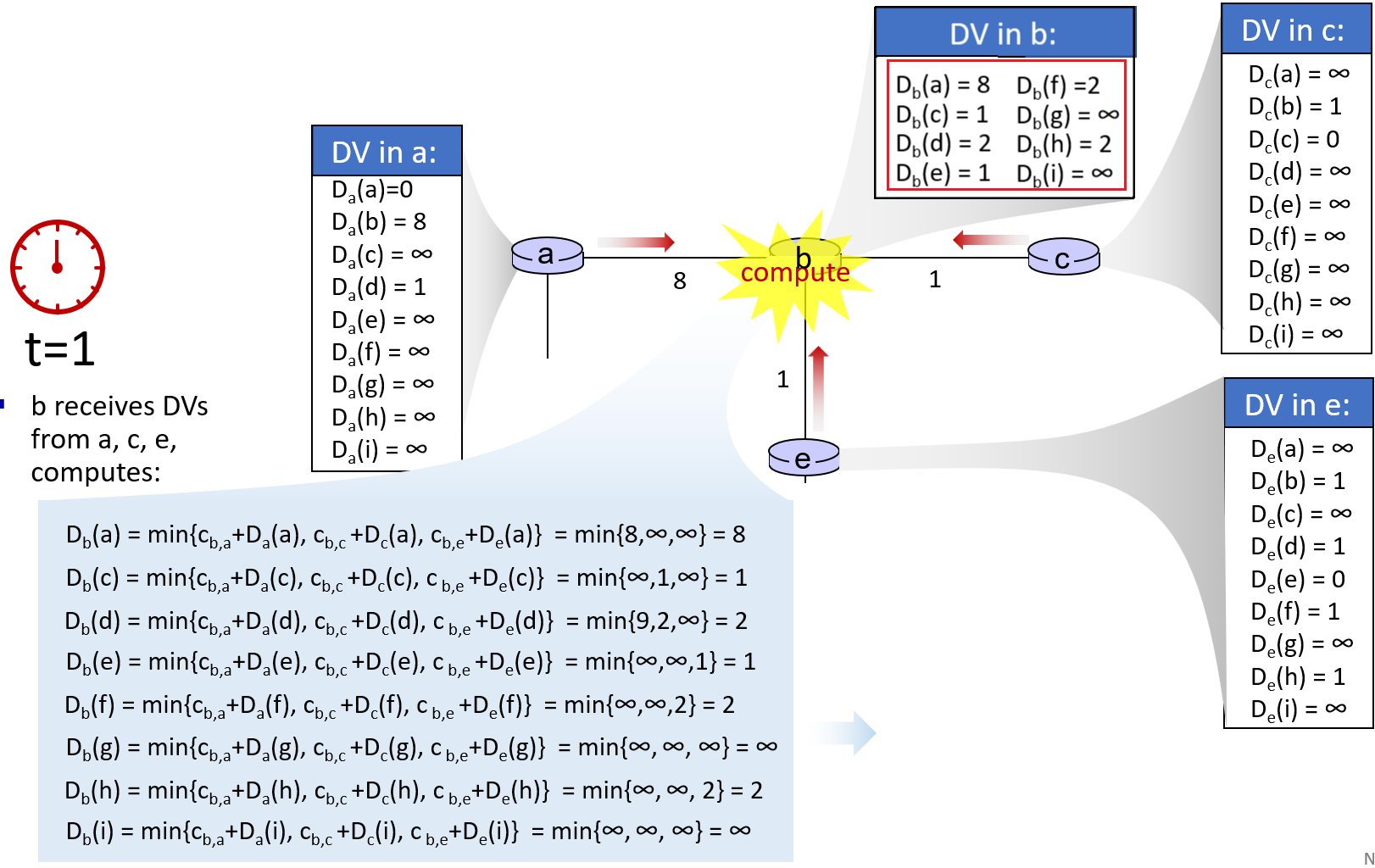 |
| Initialize the $D_x(y)$ and send | Router $b$ computes, and deliver |
where here we focused on a specific router b. In reality all other routers are also doing this action at the same time!
Link Cost Changes and Link Failure
The issue with distributed algorithm in general is their speed of convergence can be slow if there are changes!
- good news travel fast, but bad news travel very slowly! (e.g. due to change in traffic)
Case 1: Good News
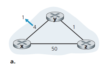
We focus here only on `y`’ and `z`’s distance table entries to destination x.
- At time $t=0$, y detects the link-cost change (the cost has changed from 4 to 1), updates its distance vector, and informs its neighbors of this change since its distance vector has changed, i.e. $D_y(x)=1$.
- At time $t=1$, z receives the update from y and updates its table. It computes a new least cost to x (it has decreased from a cost of $D_z(x)=5$ to a cost of $D_z(x)=1+D_y(x)=2$) and sends its new distance vector to its neighbors.
- here we are basically done
- At time $t=2$, y receives z’s update and updates its distance table. y’s least costs do not change and hence y does not send any message to z. The algorithm comes to a quiescent state.
Case 2: Bad News
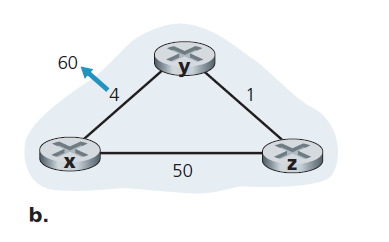
We focus here only on `y`’ and `z`’s distance table entries to destination x.
Before the link cost changes, $D_y(x) = 4, D_y(z) = 1, D_z(y) = 1$, and $D_z(x) = 5$ globally.
- At $t=0$, y detects the link-cost change (the cost has changed from $c(y,x)=4$ to $c(y,x)=60$). y computes its new minimum-cost path to x to have a cost of
which is wrong temporarily (recall that it is correct only when converged) because the only information node y has is that its direct cost to x is 60 and that z has last told y that $D_z(x)=5$, which is the wrong one.
- notice that this happens because a actually $D_z(x)=5\iff z-y-x$, but this path information is hidden/not conveyed! Now, if we picked $D_y(x)=6 \iff y - z - y -x$ will cause a routing loop for $y-z-y$ until the forwarding tables are changed.
- node y has computed a new minimum cost to x, it informs z of its new distance vector at time t1.
-
At $t=1$, z receives the update, which indicates that y’s minimum cost to x is $D_y(x)=6$. z knows it can get to y with a cost of 1 and hence computes a new least cost to x of:
\[D_z(x) = \min \{50 + 0,1 + 6 \} = 7\]which is wrong temporarily again, due to the same reason that it didn’t knw $D_y(x)=6 \iff y - z - y -x$. So z will still route through $y$.
- since z’s cost increased/changed, it sends the update to its neighbor
-
At $t=2$, y receives the update and now the path is
\[D_y(x) = \min \{ c(y,x)+D_x(x); c(y,z)+D_z(x) \} = \min \{60+0; 1+7\}= 8\]and sends to node z
-
At $t=3$, z receives the update and find $D_z(x)=9$, and etc.
Notice that at the 4rd iteration we basically successfully updated our path $D_z(x)=7+2=9$ by $2$ steps, where the correct result should be $D_z(x)=50$. Therefore, we needed $50-6=44$ iterations in total to reach the correct result.
Solution: Poisoned Reverse
The idea is simple - if z routes through y to get to destination x, i.e. $z-y-x$, then z will advertise to `y` that $D_z(x) = \infty$ (even though z knows $D_z(x) = 5$ in truth).
- basically the idea is to prevent the loop from happening, which will speed up the convergence
- z will continue telling this little white lie to y as long as it routes to x via y.
Since y believes that z has no path to x, y will never attempt to route to x via z, as long as z continues to route to x via y (and lies about doing so).
Example: Poisoned Reverse:
Now using poisoned reverse:
-
$t=0$, y knows that $D_z(x)=\infty$ (since $D_z(x)\iff z-y-x$ before, which goes through y).
Therefore, $D_y(x)=60$ on the first iteration.
- still wrong, but it converges faster
- y updates and informs its neighbor
-
$t=1$, z receives the update and now it will compute $D_z(x)=50$
- correct on the second iteration
- now $D_z(x)\iff z-x$, it does not pass through y so we can send this one to y!
-
$t=2$, y receives the update and now it gets $D_y(x)=50+1=51$!
- done
Note
Though this technique solves the current problem, it does not solve the problem completely.
- You should convince yourself that loops involving three or more nodes (rather than simply two immediately neighboring nodes) will not be detected by the poisoned reverse technique.
Comparison between LS and DV
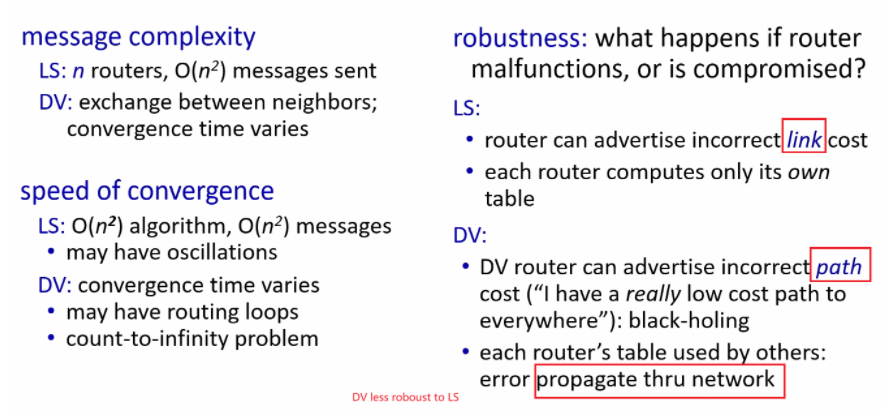
where what is important here is that:
- robustness: LS is more robust in terms of router error (e.g. router made a mistake in calculation). Since each router essentially only computes its own table, the router only causes problem to himself in LS algorithm. However, the DV algorithm would be a big problem because the error will propagate through the network and cause a vast change.
Intra-AS Routing in the Internet: OSPF
The algorithms we discussed before has a problem: each router was indistinguishable from another in the sense that all routers executed the same routing algorithm. This is not practical in reality because:
-
scalability issue: we have hundreds of millions of routers. For each router to store some table such as the DV algorithm would require enormous memory, and it will take so long that it won’t converge today
-
administrative autonomy: ISPs would like to control their routers!
Therefore, this goes back to the hierarchy setup we had in mind:
- organizing routers into autonomous systems (ASs), with each AS consisting of a group of routers that are under the same administrative control, routing algorithm and information about each other.
- then communication/exchange of information within an AS is called intra-autonomous system routing protocol
- finally, we just need to connect different AS together.
- this routing algorithm is hence called inter-autonomous system routing protocol
Hence, on a high level it looks like:
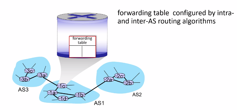
where the gateway routers (3a, 1c, 1b, and 2a) will contain entries:
- for external addresses, it sends to the external output port (decided by inter-AS-protocol)
- for internal addresses, it (decided by intra-AS-protocol)
OSPF
Open Shortest Path First (OSPF) is a link-state protocol that uses flooding of link-state information and a Dijkstra’s least-cost path algorithm.
Therefore, OSPF basically does:
- each router floods OSPF link-state advertisements (directly over IP rather than using TCP/UDP) to all other routers in entire AS
- the weights are typically set by network administrator. A simple example would be setting everything to
1, so basically it becomes the minimum hop path. - therefore, you can also customize the weights to represent information such as network delay
- the weights are typically set by network administrator. A simple example would be setting everything to
- so each router constructs a complete topological map (that is, a graph) of the entire autonomous system (not for routers outside the system!)
- When multiple paths to a destination have the same cost, OSPF allows multiple paths to be used (by splitting the traffic)
Hierarchical OSFP
In this case, we do not flood information to all routers, but in a two-level hierarchy: local area, backbone.
- link-state advertisements flooded only in area, or only in backbone
- each node has detailed area topology; only knows direction to reach other destinations
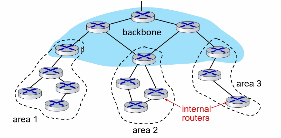
then, the last thing you need to do is to configure connection between gateway routes of your backbone and those areas.
Inter-AS Routing: BGP
Now, to route a packet across multiple ASs, we need an inter-autonomous system routing protocol.
- intra-AS algorithm completely determines the route within an AS.
Since an inter-AS routing protocol involves coordination among multiple ASs, communicating ASs must run the same inter-AS routing protocol. In fact, in the Internet, all ASs run the same inter-AS routing protocol, called the Border Gateway Protocol (BGP).
- BGP glues the thousands of ISPs in the Internet together. As we will soon see, BGP is a decentralized and asynchronous protocol in the vein of distance-vector routing
In BGP, packets are not routed to a specific destination address, but instead to CIDRized prefixes such as 138.16.68/22.
Therefore, a router’s forwarding table using BGP will include something like:
\[(\text{prefix}, \text{output})=(138.16.68/22, 3)\]where $3$ means this is for output port.
Hence BGP does two things:
- Obtain prefix reachability information from neighboring ASs. In particular, BGP allows each subnet to advertise its existence to the rest of the Internet
- Determine the “best” routes to the prefixes. A router may learn about two or more different routes to a specific prefix.
Advertising BGP Route Information
Consider the following topology, where subnet with prefix x joined Autonomous System 3.
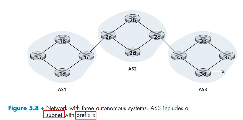
Then, to advertise x existence, we need to:
- propagate
x’s information all the way to3a, thatxis insideAS3 3atells2cin AS2 thatxis reachable viaAS3- we denote this message by
AS3-x
- we denote this message by
2cpropagate within the AS, and then gets to2a2atells1cin AS1 thatxis reachable viaAS2-AS3- we denote this message by
AS2-AS3-x
- we denote this message by
Note
For each AS, each router is either a gateway router or an internal router.
- A gateway router is a router on the edge of an AS that directly connects to one or more routers in other AS (e.g.
1c)- An internal router connects only to hosts and routers within its own AS. (e.g.
1a)
Therefore, in the above example, we see that we needed two types of BGP messages
- a BGP connection that spans two ASs is called an external BGP (eBGP) connection
- a BGP session between routers in the same AS is called an internal BGP (iBGP) connection
(so BGP exchange routing information over semi-permanent TCP connections using port 179.)
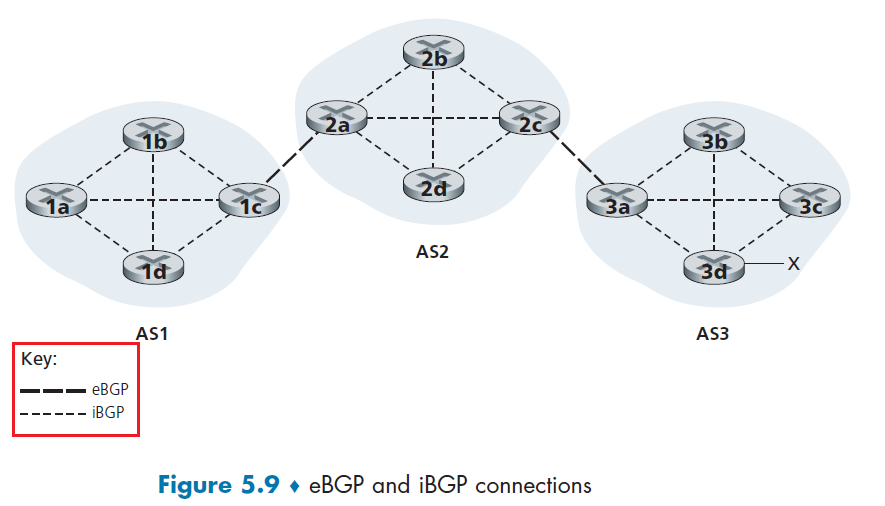
In this process,
- gateway router
3afirst sends an eBGP message “AS3 x” to gateway router2c. - Gateway router
2cthen sends the iBGP message “AS3 x” to all of the other routers in AS2, including to gateway router2a. - Gateway router
2athen sends the eBGP message “AS2 AS3 x” to gateway router1c.
So it looks more like:
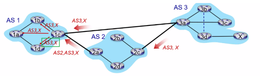
notice that:
- here the path information is a path-vector, in contract to the distance-vector which has the problem of causing loops!
Note
Here we only discussed how to get the information across. We haven’t discussed what route will then be chosen, which is the next section
Also, notice that then gateway routes need to run both eBGP and iBGP
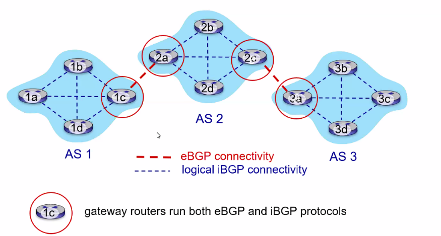
Determining the Best Routes
When BGP advertises reachability, it includes information of prefix (e.g. 138.16.68/22) + attributes.
- prefix: destination being advertised
- two of the most important attributes:
AS-PATH: list of ASN (unique ID for each AS) through which prefix advertisement has passed (contains the path information)- this is implemented by just having AS adds its ASN to the existing list in the AS-PATH
- basically this is the path vector. So BGP is Path Vector Protocol
NEXT-HOP: indicates specific internal-AS router IP to next-hop AS- because the route only contains ASN, which gave no IP information!
Other BGP Message Fields
BGP since is over TCP, contains also the following fields
OPEN: opens TCP connection to remote BGP peer and authenticates sending BGP peer
UPDATE: advertises new path (or withdraws old)
KEEPALIVE: keeps connection alive in absence of UPDATES; also ACKs OPEN request
NOTIFICATION: reports errors in previous msg; also used to close connection
For instance, consider 1d receiving advertisement to subnet with prefix x:
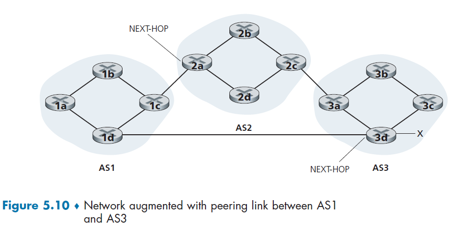
In this case, it will receive two entries:
\[\text{NEXT-HOP; AS PATH; destination prefix} = \begin{cases} \text{IP address of leftmost interface for router 2a; AS2-AS3; x}\\ \text{IP address of leftmost interface of router 3d; AS3; x} \end{cases}\]Then, with this information, we finally discuss two algorithms used for BGP routing:
- hot potato routing
- Route-Selection Algorithm
Hot Potato Routing
This is a simple algorithm where the route chosen (from among all possible routes) is that route with the **least cost to the NEXTHOP **router beginning that route.
For example, consider we wanting to send data from 1b-x. Then, if 1b uses hot potato routing:
- recall that BGP is used when we want to send data outside of AS
here we have two paths that 1b is looking at:
-
the least-cost intra-AS path to NEXT-HOP router
2a -
the least-cost intra-AS path to NEXT-HOP router
3d -
note that we need to consult intra-AS routing information!
-
e.g. from iBGP, router
1dknows1cis needed to get tox -
then from OSPF of the intra-AS algorithm,
1dknows how to get to1c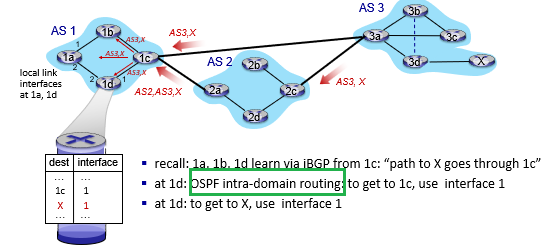
-
If the weights are all the same for intra-AS path, then:
- the least-cost intra-AS path to NEXT-HOP router
2a= 2 Hops - the least-cost intra-AS path to NEXT-HOP router
2a= 3 Hops
Hence router 2a would therefore be selected, and Router 1b would then consult its forwarding table (configured by its intra-AS algorithm) and find the interface I that is on the least-cost path to router 2a.
- then, it adds `(x, I)` to its forwarding table.
Note
reduce the cost in its own AS while ignoring the other components of the end-to-end costs outside its AS
- so in this case, we see the actual shorter path could be
AS3-xwhich goes through1d. Hence this algorithm is a bit short-sighted.
Route-Selection Algorithm
In practice, BGP uses an algorithm that is more complicated than hot potato routing, but nevertheless incorporates hot potato routing.
Recall that, for any destination prefix x.x.x.x/y, the input for BGP is the set of all routes to that prefix that have been learned and accepted by the router (rejection of a route can happen due to some policy issues)
-
- since you can reject routes, advertisement of accepted routes can also be seen as a reflection of a policy
If there are two or more routes to the same prefix, then BGP sequentially invokes the following elimination rules until one route remains:
- The routes with the highest local preference values are selected
-
A route is assigned a local preference value as one of its attributes (in addition to the AS-PATH and NEXT-HOP attributes).
-
The value of the local preference attribute is a policy decision that is left entirely up to the AS’s network administrator.
- The local preference of a route could have been set by the router or could have been learned from another router in the same AS.
- From the remaining routes (all with the same highest local preference value), the route with the shortest AS-PATH is selected.
- If this rule were the only rule for route selection, then BGP would be using a DV algorithm for path determination, where the distance metric uses the number of AS hops rather than the number of router hops.
-
From the remaining routes (all with the same highest local preference value and the same AS-PATH length), hot potato routing is used, that is, the route with the closest NEXT-HOP router is selected.
-
If more than one route still remains, the router uses BGP identifiers to select the route;
For Example
Consider the same example of Figure 5.10, where we want to send data from 1b-x.
- rule 2 is applied before rule 3, causing BGP to select the route that bypasses AS2, since that route has a shorter AS PATH.
- hence, we will select the path to
1d!
Note
In reality, BGP routing tables often contain over half a million routes, as it is the de facto for the internet today.
if
Xdisconnects, BGP will advertise a withdraw message.
Routing Policy
Here we discuss how local preferences/polices can be used to prevent unintentional network traffic flowing through due to BGP.
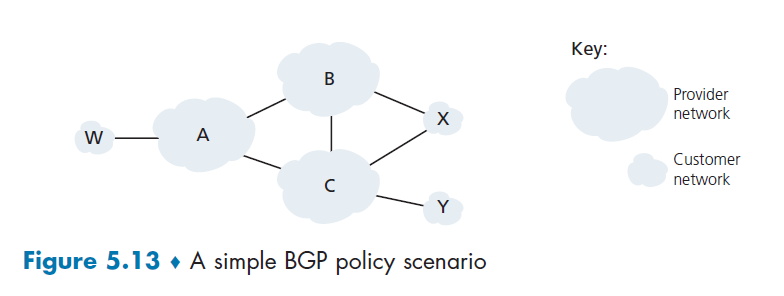
where:
- A,B,C are provider networks
- x,w,y are customer (of provider networks)
- ``x` does not want to route from B to C via x!
Then, the policy to enforce is simply advertises (to its neighbors B and C) that it has no paths to any other destinations except itself.
Another example would be to consider from B, that it wants to tell its customer x that it contains a route to w
Balso wants to advertise the pathBAWto its customer,Xso that X knows that it can route to W via B.- But
Bshould not advertise `BAW` to `C`, who would then route traffic towfromBAW!
Software Defined Network
Our study here builds on our earlier discussion of generalized SDN forwarding in Section Generalized Forwarding and SDN.
- again, here we adopt the terminology of routers are packet switches since the forwarding decisions can be made on the basis of network-layer source/destination addresses, link-layer source/destination addresses, as well as many other values in transport-, network-, and link-layer packet-header fields.
Some key characteristic of SDN:
- Flow-based forwarding. Packet forwarding by SDN-controlled switches can be based on any number of header field values (see section Generalized Forwarding and SDN with more on OpenFlow1.0)
- Separation of data plane and control plane. Recall again that now the entirety of control plane is in the remote controller in Figure 5.2. So packet switches just need to execute the “match plus action” rules in their flow tables (delivered to them by the remote controller)
- A programmable network. The network is programmable through the network control applications running in the control plane. Basically you can just program them and inject by using the Northbound API to the controllers. (Figure 5.14)
Basically the key difference is that we no longer do per-router control, such that we have a remote centralized controller.
| Overview of SDN | More Detailed SDN |
|---|---|
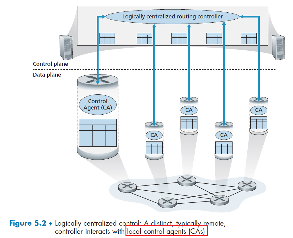 |
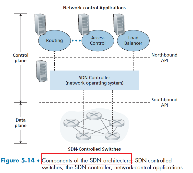 |
where:
- in Figure 5.14, control plane itself consists of two components. an SDN controller (or network operating system) and a set of network-control applications
- so it is more similar to the LS algorithm where there is a centralized agency
So SDN is really three components: data plane switches, SDN controllers, and network-control applications!
Advantage of Centralized Control
The unbundling/separation into three components gives us a rich, open ecosystem driven by innovation in all three of these areas, as now software and hardware are decoupled!
- load balancing
- those decision would go against least-weight path
- higher priority traffic to low cost and low priority to high cost link
- SDN hence used extensively for cellular networks!
so the difference from the traditional distributed algorithm becomes:
- using a centralized controller to compute table/figure out route (so control plane of routers don’t need to compute those routes)
- more functionality using flow table
SDN Controller Architecture
In short, the controller part needs to do three things:
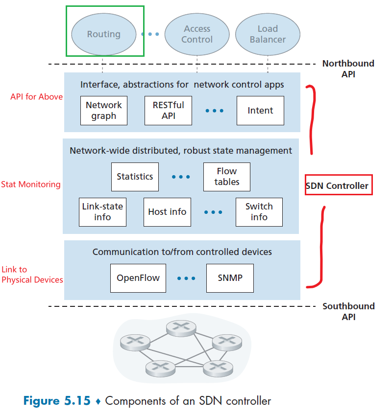
where basically:
- A communication layer: communicating between the SDN controller and controlled network devices. So here we basically have a protocol (OpenFlow or SNMP) to transfer information between the controller and that device.
- e.g. need communicating a message indicating that an attached link has gone up or down, that a device has just joined the network, or a heartbeat indicating that a device is up and operational
-
A network-wide state-management layer: basically stores state of the entire lower layer packet switches. This will be used by the upper layer “brain” software to implement load balancing and etc.
- The interface to the network-control application layer. Provide API to the software above for computation, i.e. giving the Northbound API.
Note
In this architecture, the controller plane does NOT compute route. It only maintains those route related information and it is the upper layer software that computes the route (see Figure 5.15).
OpenFlow Protocol
Here we zoom into the communication between the control layer and the packet switches below (see Figure 5.15), The OpenFlow protocol operates over TCP, with a default port number of 6653.
Among the important messages flowing from the controller to the controlled packet switch are the following:
- Configuration: controller to query and set a switch’s configuration parameters.
- Modify-State. This message is used by a controller to add/delete or modify entries in the switch’s flow table, and to set switch port properties.
- Read-State. This message is used by a controller to collect statistics and counter values from the switch’s flow table and ports.
- Send-Packet. This message is used by the controller to send a specific packet out of a specified port at the controlled switch. The message itself contains the packet to be sent in its payload.
Among the messages flowing from the SDN-controlled packet switch to the controller are the following:
- Flow-Removed. This message informs the controller that a flow table entry has been removed, e.g. due to Modify-State message
- Port-status. This message is used by a switch to inform the controller of a change in port status.
- Packet-in. Recall from section Generalized Forwarding and SDN. that a packet arriving at a switch port and not matching any flow table entry is sent to the controller for additional processing
Interaction with Network Application Layer
Here we can just walk through an example of running Dijkstra’s algorithm to figure out the shortest path among the routers.
Consider the case that router S1 and S2 link is suddenly down. Then:
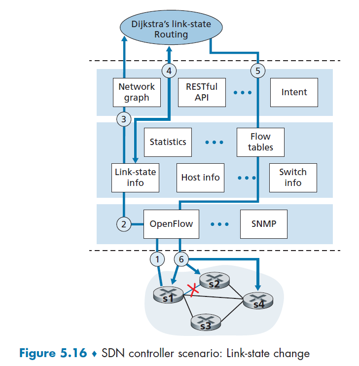
- Switch s1, experiencing a link failure between itself and s2, notifies the SDN controller of the link-state change using the OpenFlow *port-status* message
- The SDN controller receives the OpenFlow message indicating the link-state change, and notifies the link-state manager, which updates a link-state database
- The network-control application that implements Dijkstra’s link-state routing has previously registered to be notified when link state changes. That application receives the notification of the link-state change.
- link-state routing application interacts with the link-state manager to get updated link state, and perhaps also consult other components in the state-management layer for computation (e.g. Network Graph)
- application finished computing, then interacts with the flow table manager, which determines the flow tables to be updated
- The flow table manager then uses the OpenFlow protocol to update flow table entries at affected switches
SDN Challenges
- Robustness: what happens if a link between the controller and the router breaks? Then you cannot push updates/fixes!
- problem with all centralized system - single point of failure
ICMP: Internet Control Message Protocol
The ICMP is basically used for hosts and routers to communicate network-layer information to each other. This is needed especially for error reporting.
- e.g. an IP router was unable to find a path to the host specified in your HTTP request. Then that router will create and sent an ICMP message to your host indicating the error
- this example above is how you receive error message such as “Destination network unreachable.”
ICMP Messages
ICMP is often considered part of IP, but architecturally (its layer) it lies just above IP, as ICMP messages are carried inside IP datagrams.
- i.e. that is, ICMP messages are carried as IP payload, just as TCP or UDP segments are carried as IP payload
- therefore, when demultiplexing an IP packet, you can have TCP, UDP or ICMP
Now, ICMP messages typically have:
- a type and a code field (2-tuple)
- a header
- first 8 bytes of the IP datagram that caused the ICMP message to be generated in the first place
- so you know which packet caused the issue
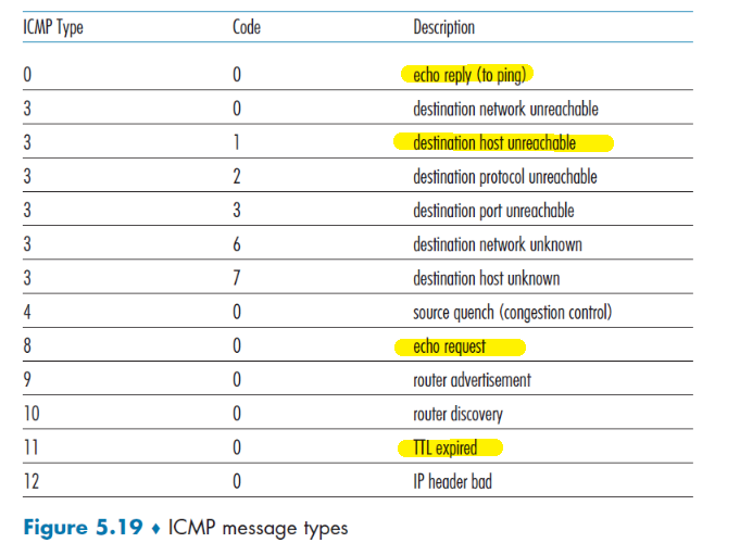
Note
- In reality the ICMP messages are usually generated by the OS directly in response to something. So there is no specific “server program” you would run.
Examples of ICMP Usages
Example: ping
The well-known ping program does this:
- client sends an ICMP type 8 code 0 message to the specified host.
- The destination host, seeing the echo request, sends back a type 0 code 0 ICMP echo reply.
Notice that, as mentioned before, most TCP/IP implementations support the ping server directly in the operating system
Example: traceroute
Traceroute is implemented with ICMP messages. As we know, basically Traceroute in the source sends a series of ordinary IP datagrams, each of these datagrams carries a UDP segment with an unlikely UDP port number.
- The first of these datagrams has a
TTLof 1, the second of 2, the third of 3, and so on - The source also starts timers for each of the datagrams
- When the $n$th datagram arrives at the $n$th router, the $n$th router observes that the TTL of the datagram has just expired.
- The router discards the datagram (according to IP protocol) and sends an ICMP warning message to the source (type 11 code 0).
- This warning message includes the name of the router and its IP address.
- When this ICMP message arrives back at the source, the source obtains the round-trip time from the timer and the name and IP address of the nth router from the ICMP message
- Repeat step 2 to 5 until received Port Unreachable ICMP Message
- Because this datagram contains a UDP segment with an unlikely port number, the final destination host sends a port unreachable ICMP message (type 3 code 3) back to the source
Network Management, SNMP, and NETCONF/YANG
Basically, here we discuss a set of network management tools and approaches that help the network administrator monitor, manage, and control the network.
- e.g. what if we want to shut down/restart a router? We cannot do what with SDN + OpenFlow as they are for routing purposes.
- here we basically discuss tools we can use to control/execute commands on a cluster of routes/devices
A brief glimps on what will be covered:
- how to communicate status information (e.g. server/router down)
- how to execute commands
In reality, as they are tools used to manage the actions (not routing) of a cluster of routers, it is very relevant to Data Center and their Software defined network.
Network Management Framework
Basically we have some network managers controlling a managing server, which can in turn collect statistics of the devices (not only routers) in the particular AS.
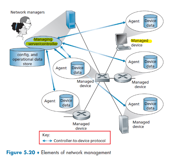
where:
- Managing server. The managing server is an application, typically with network managers (humans) in the loop, running in a centralized network management station in the network operations center (NOC). The aim is to configure, monitor, and control the network’s managed devices
- Managed device. A managed device might be a host, router, switch, middlebox, modem, thermometer, or other network-connected device.
- Data. Each managed device will have data, also known as “state.” Typically you have
- Configuration data is device information explicitly configured by the network manager. e.g. configured IP address or interface speed
- Operational data is information that the device acquires as it operates, for example, the list of immediate neighbors in OSPF protocol.
- Device statistics are status indicators and counts that are updated as the device operators
- Network management agent. The network management agent is a software process running in the managed device that communicates with the managing server.
- this is the program that actually taking local actions at the managed device under the command and control of the managing server
- Network Management Protocol. The protocol between the managing server and the devices , so that agents can use the network management protocol to
- inform the managing server of exceptional events (e.g., component failures).
- take actions as designated from the server
Then, in practise, we have three main ways where a network admin use to manage the network, using:
-
CLI. Access the device directly using command line interface, by
sshinto it. -
SNMP/MIB. Admin can query/set the data contained in a device’s Management Information Base (MIB) objects using the Simple Network Management Protocol (SNMP).
- Some MIBs are device- and vendor-specific, while other MIBs are device agnostic, i.e. generic
- this is used often in combination of CLI, i.e. you collect statistics from SNMP, and use CLI to do actions
Note that both approaches above manage devices individually.
-
NETCONF/YANG. Used for large system as it scales! It can control a collective of devices.
- NETCONF protocol [RFC 6241] is used to communicate YANG-compatible actions and data to/from/among remote devices
- YANG [RFC 6020] is a data modeling language used to model configuration and operational data.
SNMP and MIB
The Simple Network Management Protocol version 3 (SNMPv3) [RFC 3410] is an application-layer protocol used to convey network-management control and information messages between a managing server and an agent executing on behalf of that managing server.
The typical usage of SNMP is in a request-response mode in which:
- an SNMP managing server sends a request to an SNMP agent
- the SNMP agent who received the request, will perform some action and sends a response back
Another important usage is when some urgent things happened (e.g. an error):
- an SNMP agent send unsolicited message/trap message to server
So basically it looks like:
| Normal | Trap Situation |
|---|---|
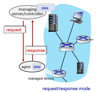 |
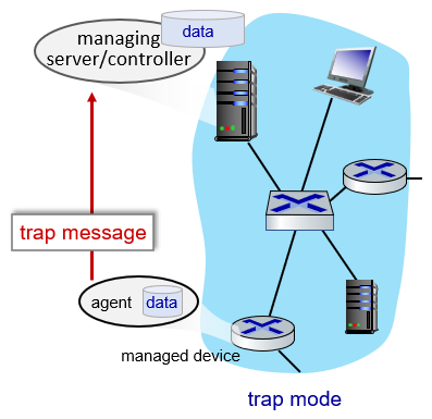 |
where:
- the left is the typical situation mentioned above, it is “triggered by server”
- the right is when something bad happened. It is “triggered by agent”
Then, SNMPv3 defines seven types of messages, known generically as protocol data units—PDUs—as shown in the table and figure below.
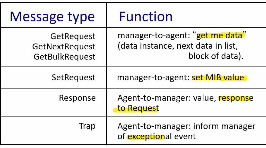
where notice that:
- the last to messages are sent from agent to manager
And a PDU that is the packet actually sent looks like
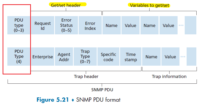
NETCONF and YANG
In this paradigm, we need managing server actively controls a managed device by sending it configurations, which are specified in a structured XML document, and activating a configuration at the managed device.
- all done in a remote procedure call (RPC) paradigm
Reminder
A remote procedure call is simply
the take-away message is that:
- for the client, it is basically asking somebody (remote) as to do the computation and return the result (execution resumes as if returning from a regular procedure call. )
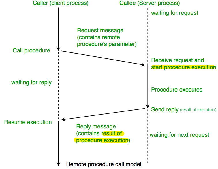
Under the hood, it is basically doing this
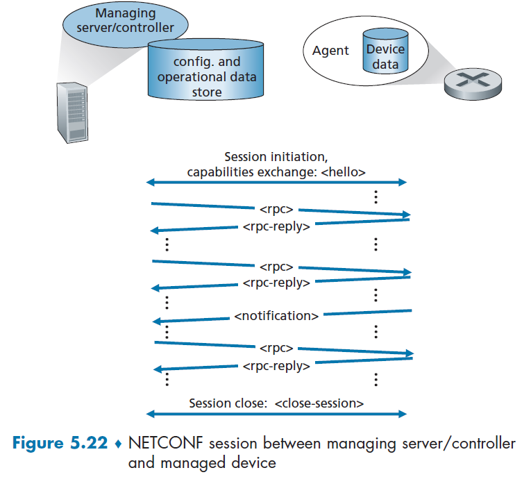
where we are using a connection-oriented session of TLS over TCP, and:
- server establishes a secure connection to the managed client (agent)
- the managing server and the managed device exchange
<hello>messages, declaring their “capabilities” - Interactions between the managing server and managed device take the form of a remote procedure call, using the
<rpc>and<rpc-response>messages.
Then some actoins that NETCONF can take is
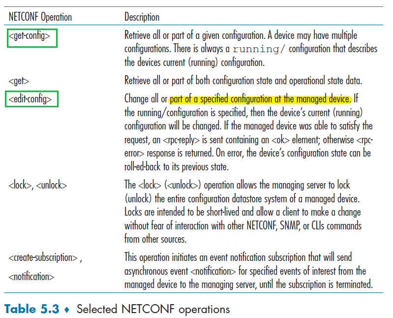
notice the emphasis on configuration of devices.
And interestingly, the actual message doing those actions are not in the format of HEADER + KEY-VALUE pairs, but now in XML format
Example: <get>
<?xml version=”1.0” encoding=”UTF-8”?>
<rpc message-id=”101”
     xmlns=”urn:ietf:params:xml:ns:netconf:base:1.0”>
    <get/>
</rpc>
where this is a NETCONF <get> command requesting all device configuration
- the RPC message itself spans lines 02–05, basically:
- RPC has a message ID value of 101
- RPC contains a single command of
<get>
Then the reply could look like
<?xml version=”1.0” encoding=”UTF-8”?>
<rpc-reply message-id=”101”
           xmlns=”urn:ietf:params:xml:ns:netconf:base:1.0”>
    <!--"."."."all configuration data returned... -->
    ...
</rpc-reply>
More complicated example:
Server wants to sets the Maximum Transmission Unit (MTU) of an interface named “Ethernet0/0” to 1500 bytes.
<?xml version=”1.0” encoding=”UTF-8”?>
<rpc message-id=”101”
     xmlns=”urn:ietf:params:xml:ns:netconf:base:1.0”>
    <edit-config>
        <target>
            <running/>
        </target>
        <config>
            <top xmlns=”http://example.com/schema/
                 1.2/config”>
                <interface>
                    <name>Ethernet0/0</name>
                    <mtu>1500</mtu>
                </interface>
            </top>
        </config>
    </edit-config>
</rpc>
where:
- RPC message itself spans lines 02–17
- contains a single NETCONF
<edit-config>command, spanning lines 04–15.
Then the reply looks like
<?xml version=”1.0” encoding=”UTF-8”?>
<rpc-reply message-id=”101”
           xmlns=”urn:ietf:params:xml:ns:netconf:base:1.0”>
    <ok/>
</rpc-reply>
YANG
YANG is the data modeling language used to precisely specify the structure, syntax, and semantics of network management data used by NETCONF.
Basic YANG then allows programmability for easier XML-based message
- variables, loops, etc to do configuration
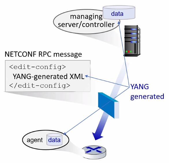
Chapter 6 Link Layer
Recap: Network layer provides a communication service between any two network hosts (by doing a bunch of routing through routers). Between the two hosts, datagrams travel over a series of communication links (routing).
Here, we consider how packets are sent across the individual links that make up the end-to-end communication path.
In particular, you will see that there are two types of link-layer channels usde to “deliver packet from one device to another” (e.g. your phone to a router)
- broadcast channels, which connect multiple hosts in wireless LANs,
- many hosts are connected to the same broadcast communication channel, a so-called medium access protocol is needed to coordinate frame transmission
- i.e. how to share the medium
- point-to-point communication link, such as that often found between two routers connected by a long-distance link, or between a user’s office computer and the nearby Ethernet switch
Introduction to the Link Layer
Here, we use the terminology that:
- refer to any device that runs a link-layer (i.e., layer 2) protocol as a node
- e.g. hosts, routers, switches, and WiFi access points
- communication channels that connect adjacent nodes along the communication path as links.
For example, sending from a laptop (host) to some server across the network:
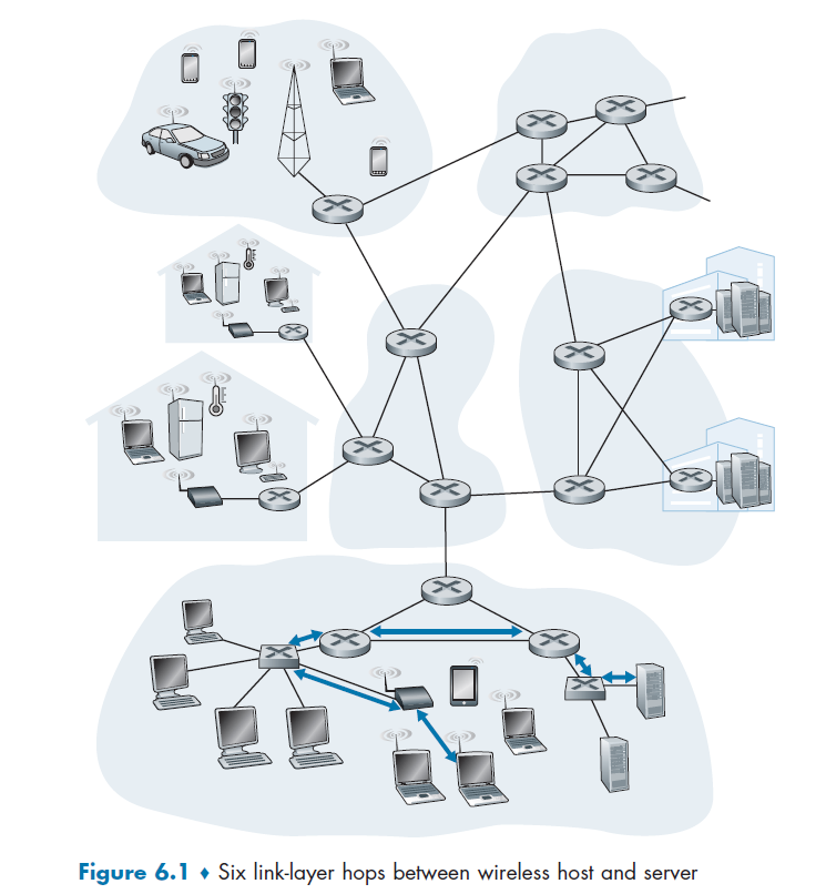
where again, we relied on the network layer to figure out the route
- then, link layer needs to deal with encapsulating IP datagram and sending it over the 6 links traversed
- notice that the first link is between a host and a wireless router!
Distinguishing between Network and Link
Consider the analogy of planning a trip for a tourist traveling from Princeton, New Jersey, to Lausanne, Switzerland.
You made a plan to
- take a limousine from Princeton to JFK airport
- then a plane from JFK airport to Geneva’s airport,
- a train from Geneva’s airport to Lausanne’s train station
then you make reservations for them as well
You actually do the trip, and then:
- Princeton limousine company to get you from Princeton to JFK;
- it is the responsibility of the airline company to get the tourist from JFK to Geneva
- it is the responsibility of the Swiss train service to get the tourist from Geneva to Lausanne
In total we got three “links”, and in particular
- you are the datagram
- travel agent deciding the route is a routing protocol (network)
- each transportation segment is a link
- the transportation mode along the route (e.g. train or plane) is a link-layer protocol
- notice that routing, in that sense, doesn’t care about how the transportation is being done. It just cares about where it is going.
- e.g. network layer ensures that Host
A-> RouterRwill work. But in reality there are many switches to reach routerRfrom host A in some subnet. Therefore, link layer deals with the delivery among switches/hosts to get to its end points (host or router)
Link Layer Services
Possible services that can be offered by a link-layer protocol include:
- Framing. Almost all link-layer protocols encapsulate each network-layer datagram within a link-layer frame before transmission over the link
- MAC addresses in frame headers identify source, destination (different from IP address!)
- Link Access. A medium access control (MAC) protocol specifies the rules by which a frame is transmitted onto the link. Basically the two cases that:
- if there is only a point-to-point link, i.e. a single sender and a receiver, then MAC is simple or nonexistent
- The more interesting case is when multiple nodes share a single broadcast link—the so-called multiple access problem. Here, the MAC protocol serves to coordinate the frame transmissions of the many nodes.
- Reliable Delivery. First note that this is different from the higher layer reliable deliver such as TCP (host to host). Here, the the aim is to guarantees to move each network-layer datagram across the link without error (node to node).
- in the end, it is the achieved the same with acknowledgments and retransmissions (see Section 3.4).
- this is often used for links that are prone to high error rates, such as wireless link, so that error are corrected immediately/locally (as compared to realizing only at the destination host that something is wrong). Links with low error rates such as fiber do not typically use this, so there is a less overhead.
- Error detection and Correction. Bits are basically electric signals, so bit error can occur due to attenuation and electromagnetic noise. If error can be discovered fast, then we don’t waste time to forward it all the way to destination.
- This is done by having the transmitting node include error-detection bits in the frame, and having the receiving node perform an error check. (more sophisticated than checksum)
Recall
Each time for a single message to be exchanged, you went:
- from application layer all the way down to physical of a host (when sending)
- from physical layer all the way up to application layer of a host (when received)
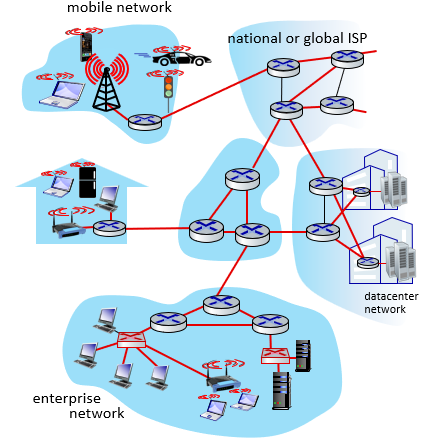
where basically the red parts are the link-layer’s job.
Where Is the Link Layer Implemented
Link layer is basically implemented in every device in the network that can communicate/send/switch packets.
In a host, e.g. your laptop link layer is implemented on a chip called the network adapter
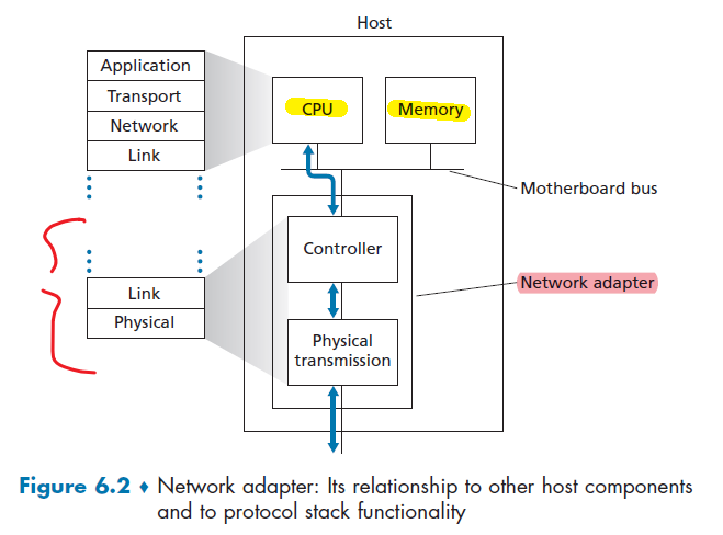
where:
- the network adapter is sometimes known as a network interface controller (NIC).
- Thus, much of a link-layer controller’s functionality is implemented in hardware (controller).
- part of the link layer is implemented in software that runs on the host’s CPU, e.g. handling controller interrupts when received data.
- for a sender, the controller
- takes the datagram created/ready from the memory
- encapsulate it into an link-layer frame
- potentially setting error detection bits as well
- transmit it into the physical transmissions part
- for a receiver, then controller
- receive the tram from the link
- extract the network layer datagram
- potentially perform error detection
- puts it in the memory and informs CPU that data is received
Error Detection and Correction
In this section, we’ll examine a few of the simplest techniques that can be used to detect and, in some cases, even fix the bit error.
- so here we assume (and this is commonly done anyway) that sender configured the error-detection and -correction bits (EDC).
Essentially, given the new frame D', EDC':
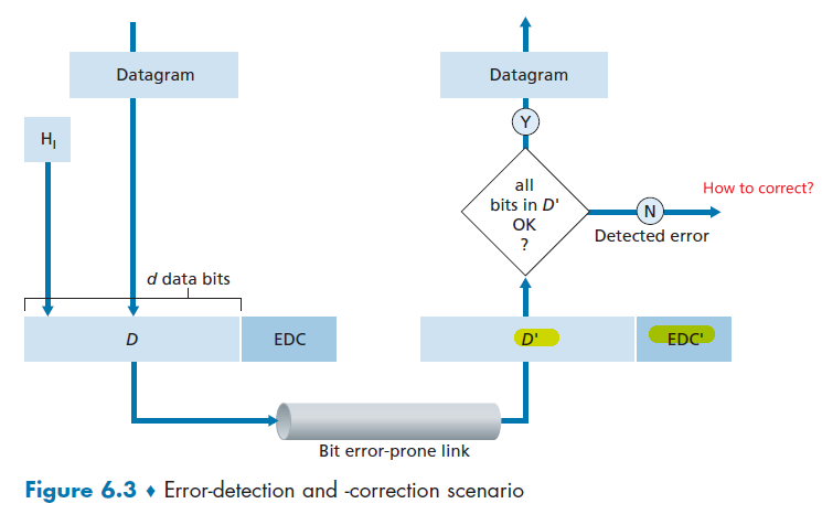
where:
- notice that
EDC'might also be flipped - We thus want to choose an error-detection scheme that keeps the probability of “receiving a corrupted packet and not noticing” to be small.
- there is always the case that everything could go wrong, so we want to keep the probability of that small
Parity Checks
Perhaps the simplest form of error detection is the use of a single parity bit. Here you have two schemes to choose from (basically same idea)
Let the entire information to be sent, $D$, include $d$ bits.
-
Using an even parity scheme:
The sender simply includes one additional bit and chooses its value such that the total number of 1s in the $d + 1$ bits (including the parity bit) is even.
- i.e. put $1$ if there were odd number of 1s in the $d$ bits. Otherwise, put $0$.
-
Using an odd parity scheme
The sender includes the parity bit such that there is an odd number of $1$s in the $d+1$ bits.
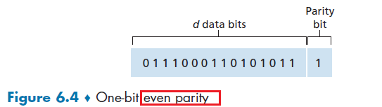
However, this is not used in reality because:
- multiple errors often happen in a cluster. So sometimes error become undetected as you only used 1 bit for error
- it was shown that under burst error condition, this could happen about 50 percent of the time
- no idea how to correct the error, as you don’t know where the error is.
But this idea is not useless. Consider using a two-dimensional generalization of the single-bit parity scheme.
- Here, the $d$ bits in $D$ are divided into $i$ rows and $j$ columns.
- A parity value is computed for each row and for each column.
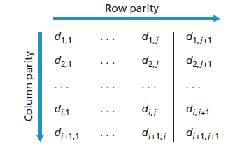
where:
- the $d_{i+1,j+1}$ is the parity bit for that parity bits’ column and row
Then, this is possible to detect and CORRECT a single bit error.
| No Error | Error Detected |
|---|---|
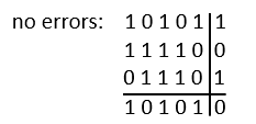 |
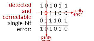 |
where we assumed that we are using even parity
- if there is a single bit error in the data, it is detectable and correctable
- if there is a single bit error in the parity bits, it is also detectable and correctable
- if there are two errors, this can only detect but not correct the errors.
Forward Error Correction (FEC)
The ability of receiver to both detect and correct errors is known as forward error correction (FEC).
- again, those FEC techniques are valuable because they can decrease the number of sender retransmissions required. Perhaps more important, they allow for immediate correction of errors at the receiver, instead of waiting for an entire round-trip propagation delay.
Checksumming Methods
In checksumming techniques, the $d$ bits of data in Figure 6.4 are treated as a sequence of $k$-bit integers (e.g. $k=16$ for the Internet Checksum)
- for $k=16$, then bytes of data are treated as 16-bit integers and summed
Basically for sender, the checksum is computed by taking 1’s complement of the sum of data:
- 1’s complement is basically inverting all the bits in the binary representation
              10101001
              00111001
              --------
   Sum        11100010
   Checksum:  00011101
Then, the checksum is used by receiver so that summing all of them (including checksum) and taking 1’s complement should give you all 0s.
			   10101001
               00111001
               00011101 // checksum
               --------
   Sum         11111111
   Complement  00000000  means that the pattern is O.K.
Again, this is fast but does not tell you where the error is. So it cannot be corrected.
Note
Checksumming methods require relatively little packet overhead. However, they provide relatively weak protection against errors as compared with cyclic redundancy check. But the question is then why is TCP and UDP not using cyclic redundancy check?
- Because transport-layer error detection is implemented in software, it is important to have a simple and fast error-detection scheme such as checksumming.
- On the other hand, error detection at the link layer is implemented in dedicated hardware in adapters, which can rapidly perform the more complex CRC operations.
Cyclic Redundancy Check (CRC)
CRC codes operate as follows. Consider the $d$-bit piece of data, $D$, that the sending node wants to send to the receiving node. The sender and receiver must first agree on an $r + 1$ bit pattern, known as a generator, which we will denote as $G$.
- ofc we need the most significant (leftmost) bit of $G$ be a $1$.
Then, the idea is as follows:
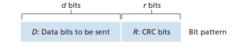
- For a given piece of data, $D$, the sender will choose $r$ additional bits, $R$, and append them to $D$ such that the resulting $d + r$ bit pattern (interpreted as a binary number) is exactly divisible by $G$
- The receiver divides the $d + r$ received bits by $G$. If the remainder is nonzero, the receiver knows that an error has occurred
Then, how do we come up with the $R$?
All CRC calculations are done in modulo-2 arithmetic without carries in addition or borrows in subtraction. Same case for division and multiplication.
Therefore:
addition and subtraction are the same, and both are the same as XOR operation
1011 - 0101 = 1110
1011 + 0101 = 1110
and XOR:
1011 XOR 0101 = 1110division and multiplication in binary basically does:
multiplication by $2^k$ left shifts a bit pattern by $k$ places
an example of division looks like the follows
where basically:
\[101110000 \div 1001 = 101011 ... 011\]where $R=011$ is a remainder.
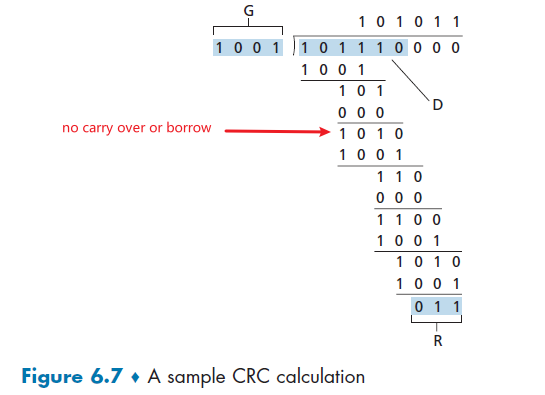
Now, given the division above, you will see that what is sent is eventually:
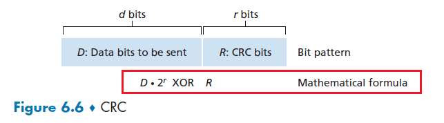
In other words, choose $R$ such that:
\[nG = D \cdot 2^r - R = D \cdot 2^r \text{ XOR } R\]where $G,r,D$ are given in the setup. So our task is to *figure out what is $R$., such that our data is divisible by $G$.
Then, since we know $(A \text{ XOR }B) \text{ XOR }B = A$, then:
\[\begin{align*} D \cdot 2^r \text{ XOR } R &= nG\\ D\cdot 2^r &= nG \text{ XOR } R\\ \text{remainder} \frac{D\cdot 2^r}{G} &= R \end{align*}\]where the last equality comes from the fact that $D\cdot 2^r= nG \text{ XOR } R$ means $R$ is the remainder if you divide $D\cdot 2^r$ by $nG$.
- see Figure 6.7 above which basically has $r=3$, $G=1011$ and $D=1011101$ as an example.
Note
- recall that $r$ is fixed, and $G$ is a given $r+1$ bit pattern. Only $R$ is computed.
- This can detect all burst errors less than $r+1$ bits (i.e. any error formed with $r$ consecutive bits or fewer will be detected)
International standards have been defined for 8-, 12-, 16-, and 32-bit generators, $G$. The CRC-32 32-bit standard, which has been adopted in a number of link-level IEEE protocols, uses:
\[G_{CRC-32} = 100000100110000010001110110110111\]where
- in addition to detect any $r$ bit or fewer consecutive errors, each of the CRC standards can detect any odd number of bit errors
Multiple Access Links and Protocols
Recall
We have two types of network links:
- A point-to-point link: consists of a single sender at one end of the link and a single receiver at the other end of the link.
- Many link-layer protocols have been designed for point-to-point links; the point-to-point protocol (PPP) and high-level data link control (HDLC) are two such protocols
- this is simple, so not discussed here
- broadcast link: multiple host wants to send and receive connected to the same single shared broadcast channel
- discussed below
- the term broadcast is used because when a node sends stuff, all the other node can “hear”/receive that
Consider you are the teacher (i.e. wireless router) in the classroom, and your students (i.e. hosts such as laptops, phones) want to ask some questions (transmit data to you). Then, the problem is:
- to receive something, a student needs to speak up
- if more than one student speaks up, you cannot hear what is happening as voice overlaps
- the broadcast channel in this case is the classroom
| Analogy | Shared Wireless |
|---|---|
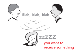 |
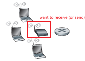 |
So the problem is how to coordinate the access of multiple sending and receiving nodes to a shared broadcast channel—the multiple access problem.
- i.e. signals of the colliding frames become inextricably tangled together when more than two nodes are transmitting at the same time (again, because (radio) waves is used to transmit information for WiFi, so it is broadcasted and can be mingled with others.)
- note one crucial difference with the classroom analogy is that, a teacher can see AND hear students (e.g. raising hand). However, a wireless router can only hear, i.e. everything happens within the same single channel. Your data channel and control channel is the same is causing more problem!
To solve this issue, computer networks have protocols—so-called multiple access protocols. In the ideal case, we want the following to happen when there is a shared/broadcast channel with multiple nodes:
- When only one node has data to send, that node has a throughput of $R$ bps.
- When $M$ nodes have data to send, each of these nodes has a throughput of $R/M$ bps.
- This need not necessarily imply that each of the M nodes always has an instantaneous rate of R/M, but rather that each node should have an average transmission rate of $R/M$ over some suitably defined interval of time.
- The protocol is decentralized; that is, there is no master node that represents a single point of failure for the network.
- The protocol is simple, so that it is inexpensive to implement.
Until today, over many years of research, we have made many working protocols for multiple access links, and they can be classified in general to the following three classes:
- channel partitioning
- divide channel into smaller “pieces” (time slots, frequency, code)
- allocate piece to node for exclusive use
- random access
- channel not divided, allow collisions
- “recover” from collisions by asking each node to randomly retransmit
- “taking turns”
- nodes take turns, but nodes with more to send can take longer time in a turn
Channel Partitioning
Basically there are two protocols used: TDM which divides by timeslot, and FDM which divides by frequency.
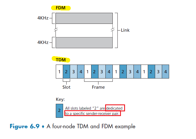
For the below discussion, let channel supports $N$ nodes and that the transmission rate of the channel is $R$ bps.
TDMA: time division multiple access
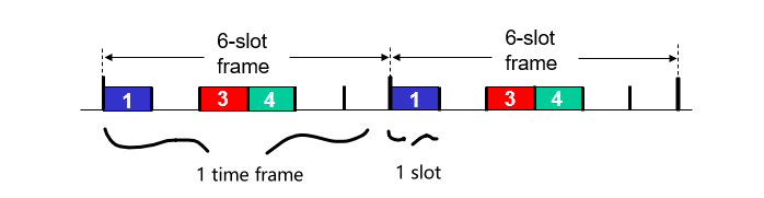
- TDM divides time into time frames (nothing to do with “frame” of a link layer packet) and further divides each time frame into $N$ time slots
- Each time slot is then assigned to one of the $N$ nodes.
- slot sizes are chosen so that a single packet can be transmitted during a slot time.
Therefore, it is fair in that each node gets a dedicated transmission rate of $R/N$ bps during each frame time. However, some obvious problems is:
- unused slots go idle, waste to time slot/efficiency
- a node is limited to only $R/N$ rate even if someone is not sending stuff
- a node must always wait for its turn in the transmission sequence—again, even when it is the only node with a frame to send.
FDMA: frequency division multiple access
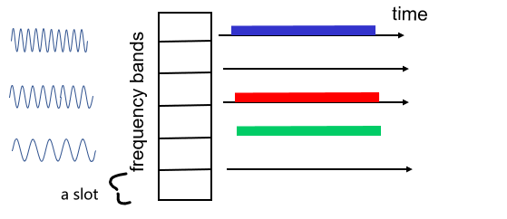
- FDM divides the $R$ bps channel into different frequencies (each with a bandwidth of $R/N$)
- assigns each frequency to one of the $N$ nodes.
Again, it avoids collisions and divides the bandwidth fairly among the $N$ nodes, but:
- a node is limited to a bandwidth of $R/N$, even when it is the only node with packets to send.
Random Access Protocol
The basic principle between protocols under this category is:
- no coordination, node always transmits at the full rate of the channel, namely, $R$ bps.
- then two or more nodes transmitting at the same time, we have a “collision”. (otherwise done)
- Then each node repeatedly retransmits its frame (that is, packet) until its frame gets through without a collision.
- in fact, there will be a random delay before retransmitting the frame, whose mechanism will be decided by the specific protocol.
- however, it is kind of like “hope and pray”, as there is a chance that both nodes still picked the same delay
Slotted ALOHA
Our following discussion assumes the following:
- All frames consist of exactly $L$ bits.
- Time is divided into slots of size $L/R$ seconds (that is, a time slot equals the time to transmit one frame).
- Nodes start to transmit frames only at the beginnings of slots.
- so nodes’ clocks are synchronized so that each node knows when the slots begin.
- If two or more frames collide in a slot, then all the nodes detect the collision event before the slot ends.
Operation: Let $p$ be a probability configured beforehand (optimal $p^*$ discussed below). Then:
- when node obtains fresh frame, waits until the beginning of the next slot and transmit
- if no collision: success and done
- if collision: node retransmits frame in each subsequent slot with probability $p$ until success
- i.e. in each subsequent slot, toss the biased coin with $p$ and decide whether to retransmit
- hopefully, eventually only one node will transmit within a slot - success
Some advantages include:
- slotted ALOHA allows a node to transmit continuously at the full rate, $R$, when there is only one active node
- highly decentralized, because each node detects collisions and independently decides when to retransmit
- yet clocks needs to be synchronized
- simple to implement
Some problems:
-
many time slots will be wasted if more than one active nodes:
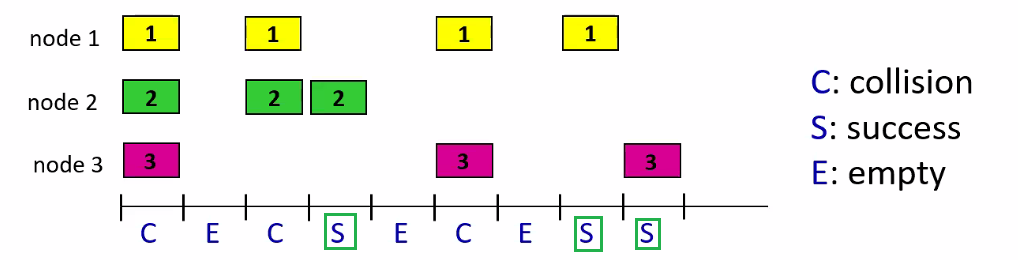
in this example, only 3 slots were “successful”, and 6 were wasted.
We can in fact compute the efficiency (which is $1/e\approx 0.37$, and then derive the optimal $p^*$.
Efficiency of a slotted multiple access protocol
This efficiency is defined to be the long-run fraction of successful slots in the case when there are a large number of active nodes.
To keep the derivation simple, assume that each node always has a frame to send and that the node transmits with probability $p$ for a fresh frame as well as for a frame that has already suffered a collision.
Then, we know that:
- the probability one given node has a success is $p(1 - p)^{N-1}$, i.e. only one decided to retransmit
- Because there are $N$ nodes, the probability that any one of the $N$ nodes has a success is $Np(1 - p)^{N-1}$. (multiply by ${n \choose 1} = N$)
Therefore, efficiency with $N$ active nodes is:
\[Np(1 - p)^{N-1}\]Let $p^*$ be the probability that maximizes this:
- take derivatives to find best $p^*$
- take $\lim_{N \to \infty}$ with $p^*$ to find maximum efficiency
Then, you will find that maximum efficiency of the protocol is given by $1/e \approx 0.37$.
- when a large number of nodes have many frames to transmit, then (at best) only 37 percent of the slots do useful work
- the effective transmission rate of the channel is not $R$ bps but only $0.37 R$ bps
Pure ALOHA
Basically without the slotted ALOHA without clock synchronization, such that they transmit/retransmit immediately if coin toss is successful.
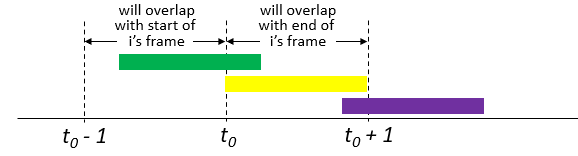
Operation
- when a frame first arrives, the node immediately transmits the frame in its entirety into the broadcast channel
- if collided, the node will then immediately (after completely transmitting its collided frame) toss a coin with probability $p$ and then retransmit the frame if coin said yes
Now, what is the effiency and the best $p^*$? Intuitively it must be less than the slotted ALOHA due to non-coordination (the efficiency is only $1/(2e) \approx 18\%$.
Then, consider:
-
given one node transmitted successfully when it started at $t_0$. This means that:
- no other node transmitted during $[t_0 - 1, t_0]$, this happens with $(1-p)^{N-1}$
- no other node begins transmission during $[t_0, t_0+1]$. This happens also with $(1-p)^{N-1}$
therefore, it is successful only when both events happen, hence one node success is:
\[(1-p)^{2(N-1)}\] -
then for $N$ nodes, multiply this by ${n \choose 1} = N$
Finally by taking limits as in the slotted ALOHA case, we find that the maximum efficiency of the pure ALOHA protocol is only $1/(2e)$.
CSMA
This basically tries to address one simple optimization of the previous protocols: if you see someone transmitting, you know a collision will happen so you should stop wasting your time trying it!
-
Listen before speaking. If someone else is speaking, wait until they are finished. In the networking world, this is called carrier sensing— listens to the channel before transmitting
- i.e. begin transmission only if it hears no one speaking
-
If someone else begins talking at the same time, stop talking. In the networking world, this is called collision detection. This can still happen as it takes time for one’s voice to reach the other.
-
e.g. if you have 4 nodes, two nodes $B,D$ wants to transmit something
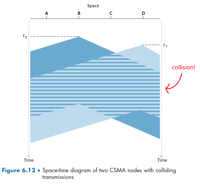
notice that $t_0$, $B$ didn’t hear anything, and at $t_1$, $D$ also didn’t hear anything yet.
-
Operation: CSMDA (without collision detection)
- a node listens to the channel before transmitting.
- if it detects no transmissions for a short amount of time, start transmitting
- If it detects that another node is transmitting an interfering frame (e.g. Figure 6.12 collision)
- it waits until transmission finished (no abort)
- waits a random amount of time before repeating the sense-and-transmit-when-idle cycle.
As shown in Figure 6.12, performance of this protocol will be greatly affected by the channel’s propagation delay.
- The longer this propagation delay, the larger the chance that a carrier-sensing node is not yet able to sense a transmission that has already begun at another node in the network.
CSMA/CD
Basically here we add the abortion to CSMA, so it is added CD for collision detection.
Operatoin:
- a node listens to the channel before transmitting.
- if it detects no transmissions for a short amount of time, start transmitting
- While transmitting, the adapter monitors for the presence of signal energy coming from other adapters using the broadcast channel
- If it detects that another node is transmitting an interfering frame, abort transmission.
- After aborting, the adapter waits a random amount of time (otherwise forever collision) and then returns to step 1.
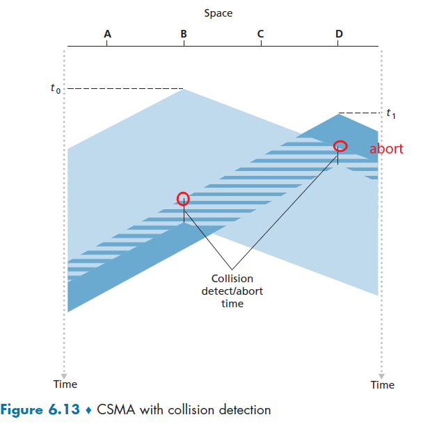
In this way, we can basically start the next cycle of wait and transmit earlier = more efficient. But one problem is what is a good interval of time for backoff (after abort)?
- If the interval is large and the number of colliding nodes is small, nodes are likely to wait a large amount time = wasted
- if the interval is small and the number of colliding nodes is large, it’s likely that the chosen random values will be nearly the same, and transmitting nodes will again collide.
Binary Exponential Backoff Algorithm
when transmitting a frame that has already experienced $n$ collisions, a node chooses the value of $K$ at random from:
\[\{0,1,2,..., 2^{n}-1\}\]where the maximum/range it can choose grows exponentially.
- thus, the more collisions experienced by a frame, the larger the interval from which $K$ is chosen.
- For Ethernet, the actual amount of time a node waits is $K \cdot 512$ bit times (i.e., $K$ times the amount of time needed to send 512 bits into the Ethernet)
Example
Suppose that a node attempts to transmit a frame for the first time and while transmitting it detects a collision.
- The node then chooses $K = 0$ with probability $0.5$ or chooses $K = 1$ with probability $0.5$.
- If the node chooses $K = 0$, then it immediately begins sensing the channel.
- If the node chooses $K = 1$, it waits $512$ bit times (e.g., 5.12 microseconds for a 100 Mbps Ethernet) before beginning the sense-and-transmit-when-idle cycle.
- After a second collision, $K$ is chosen with equal probability from ${0,1,2,3}$.
- After three collisions, $K$ is chosen with equal probability from ${0,1,2,3,4,5,6,7}$.
- etc.
Efficiency of CSMA/CD
Basically derivattion is skipped, and we were computing for the long-run fraction of time during which frames are transmitted without collisions.
\[\text{Efficiency} = \frac{1}{1+5d_{\mathrm{prop}}/d_{\text{trans}}}\]where:
- $d_{\mathrm{prop}}$ is the maximum time it takes for a signal energy to propagate between two adapters
- $d_{\mathrm{trans}}$ is the time to transmit a maximum size frame
- if $d_{\mathrm{prop}} \to 0$, then efficiency is $1$.
- as $d_{\mathrm{trans}}$ becomes very large, efficiency approaches 1. This is also intuitive because when a frame grabs the channel, it will hold on to the channel for a very long time;
Taking-Turns Protocols
Recall that two desirable properties of a multiple access protocol are
- when only one node is active, the active node has a throughput of $R$ bps
- when $M$ nodes are active, then each active node has a throughput of nearly $R/M$ bps.
Both ALOHA and CSMA can only achieve the first but not the second. This creates the desire for those taking-turns protocols which basically tries to round-robin among the nodes.
Here we introduce two protocols:
- polling protocol
- token-passing protocol
Polling Protocol Operation
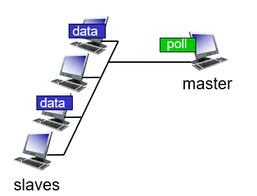
- one of the nodes to be designated as a master node
- master node polls each of the nodes in a round-robin fashion.
- master node first sends a message to node 1, saying that it (node 1) can transmit up to some maximum number of frames
- After node 1 transmits some frames, the master node tells node 2 it (node 2) can transmit up to the maximum number of frames.
- master node can determine when a node has finished sending its frames by observing the lack of a signal on the channel
- Repeats step 2 to 3 in a cyclic manner
We notice that even though it “eliminates” the collisions and empty slots that plague random access protocols, it! also has a few drawbacks:
-
introduces a polling delay—the amount of time required to notify a node that it can transmit. Therefore, technically the transmission is less than $R$ bps if only one active node.
-
(single point of failure) if the master node fails, the entire channel becomes inoperative.
Token-Passing Protocol
No master node, but a small, special-purpose frame known as a token is exchanged among the nodes in some fixed order.
- node 1 holds the token, can transmit if needed. If not, always send the token to node 2.
- If a node does have frames to transmit when it receives the token, it sends up to a maximum number of frames
- repeat step 1
Token passing is decentralized and highly efficient, but again problems can occur:
- the failure of one node (e.g. losing the token) can crash the entire channel.
DOCSIS: Protocol for Cable Access
A cable access network will make for an excellent case study here, as we’ll find aspects of each of these three classes of multiple access protocols with the cable access network!
Recall that the basic architecture looks like
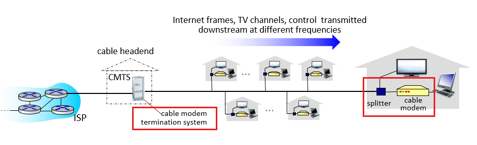
where
- cable access network typically connects several thousand residential cable modems to a cable modem termination system (CMTS) at the cable network headend.
- The Data-Over-Cable Service Interface Specifications (DOCSIS) [DOCSIS 3.1 2014; Hamzeh 2015] specifies the cable data network architecture and its protocols.
In a simpler view:
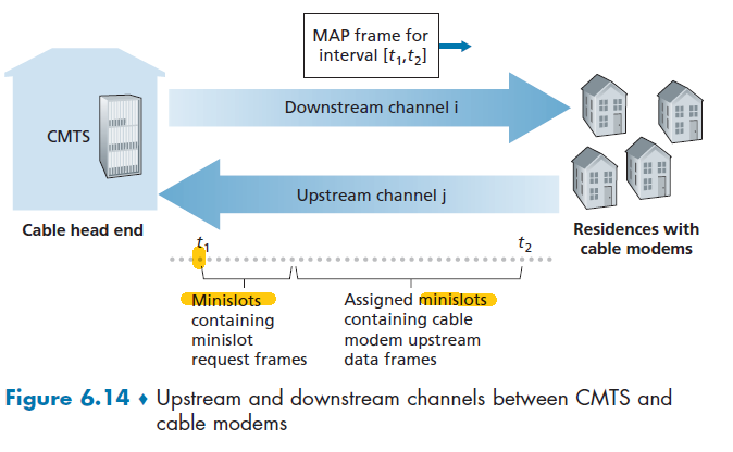
where:
- Each upstream and downstream channel is a broadcast channel, so we need to consider multiple access!
- since there is just a single CMTS transmitting into the downstream channel, this is technically easy
- DOCSIS uses FDM to divide the downstream (CMTS to modem) and upstream (modem to CMTS) network segments into multiple frequency channels.
- first partition the single channel into multiple channels, so we can split downstream and upstream
- Then, each upstream channel is further divided into intervals of time (TDM-like), each containing a sequence of mini-slots during which cable modems can transmit to the CMTS.
- For a cable modem to send upstream, it needs to:
- send mini-slot-request frames to the CMTS during a special set of interval mini-slots that are dedicated for this purpose (the ones on the front in Figure 6.14)
- the mini-slot-request frames are transmitted in a random access manner and so may collide with each other
- cable modems has no collision detection ability, so it only infer a collision if it did not receive a response
- When a collision is inferred, a cable modem uses binary exponential backoff
- CTMS responds to the requests by sending a MAP message. Basically each message explicitly grants permission to individual cable modems to transmit during specific mini-slots as specified in the MAP message.
- taking-turns alike strategy, so CMTS can ensure there are no colliding for data upstream.
Switched Local Area Network
Figure 6.15 shows a! switched local network connecting three departments, two servers and a router with! four switches.
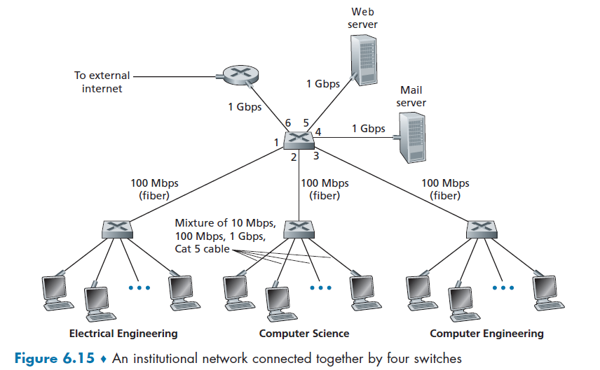
where here:
- switches operate at the link layer, so they switch link-layer frames
- those switches don’t recognize network-layer addresses (IP address), and don’t use routing algorithms like OSPF to determine the path.
- it might be confusing first why we needed two addresses, MAC and IP, but the rest of this sectoin should clarify
Link-Layer Addressing and ARP
We know that Hosts and routers have network-layer IP addresses. But it turns out that they also have link-layer addresses.
- you will see why the two layers of addresses are useful and, in fact, indispensable.
- basically imaging IP address as your post address, which changes as you move, MAC address as your SSN/ID actual identity
it is not hosts and routers that have link-layer addresses but rather their adapters (that is, network interfaces) that have link-layer addresses (MAC address)
MAC Addresses
We know that for layer 3 (network) and above, we use MAC address
- link-layer address is variously called a LAN address, a physical address, or a MAC address
- the MAC address is 6 bytes long, giving $2^{48}$ possible MAC addresses.
- typically expressed in hexadecimal notation, with each byte of the address expressed as a pair of hexadecimal numbers.
- no two adapters have the same address. It is globally unique. (IEEE manages the MAC address space)
E.g. a MAC address could look like:
\[\text{1A-2F-BB-76-09-AD }\]moreover:
- An adapter’s MAC address has a flat structure (as opposed to a hierarchical structure) and doesn’t change no matter where the adapter goes
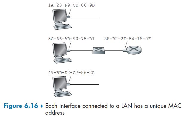
notice that a switch has no MAC addresses, but routers/hosts do.
When an adapter wants to send a frame to some destination adapter:
- the sending adapter inserts the destination adapter’s MAC address into the frame
- sends the frame into the LAN with switches
- sometimes, switches will broadcast a frame to all interfaces. So, when an adapter receives a frame, it will check to see whether the destination MAC address matches its own.
- if a sending adapter does want all the other adapters on the LAN to receive and process the frame it is about to send. In this case, the sending adapter inserts a special MAC broadcast address into the destination address field of the frame: $\text{FF-FF-FF-FF-FF-FF}$
- switches do something (see below)
The basic function of a switch is transparent bridging - for this, it doesn’t need any MAC address of its own
- Transparent bridging does not alter the frame. Layer 2 switches do not need the base Ethernet MAC address of the device nor its switch port MAC addresses to operate.
- The source and destination MAC addresses of the incoming frame are examined, the first one being saved in the MAC address table along with the receiving port, while the destination MAC address being looked up in the MAC address table to see if there is an associated port.
- If there is the frame is forwarded out that port only, otherwise it gets broadcast out all ports, except the source port (split horizon rule).
Note that:
- in the second step, we needed MAC address to check if packet belongs to us. This is the same situation in real life as IP=postal address and MAC=actual identity.
- some packages (e.g. from Amazon) might end up at your postal address
- you (MAC address) check if it is really belonging to you (could belong to the previous person living here)
- how a switch knows where to send is covered in section Link-Layer Switches
Now, the question is, how do you know what is the MAC address of a destination adapter?
ARP: Address Resolution
How do we know the MAC address given an IP address?
- This problem occurs because lower layer (link layer) uses MAC address to identify each other, instead of IP.
Then, basically you need some broadcasting to query information, using the Address Resolution Protocol (ARP).
ARP resolves IP addresses only for hosts and router interfaces on the same subnet
- to see what to do when sending across subnets, see next section.
For this example, we assume transmitting within the same subnet. Now, suppose that the host with IP address 222.222.222.220 wants to send an IP datagram to host 222.222.222.222:
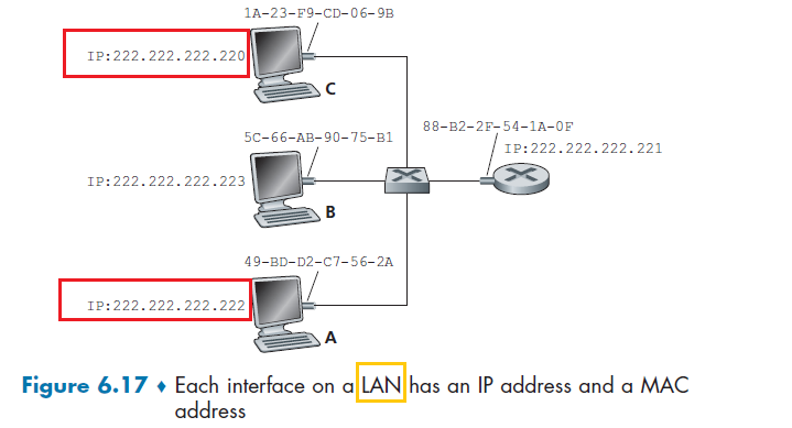
-
The sending adapter will then construct a link-layer frame, put its own MAC address as source, and need to figure out the destination’s MAC address
-
Each host and router has an ARP table in its memory, which contains mappings of IP addresses to MAC addresses.
For
222.222.222.220, it might have: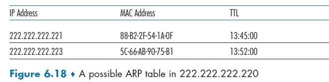
-
Using ARP protocol, first the sender constructs a special packet called an ARP packet.
- including the sending MAC addresses and receiving IP address as $\text{FF-FF-FF-FF-FF-FF}$
- The purpose of the ARP query packet is to query all the other hosts and routers on the subnet to determine the MAC address corresponding to the IP address that is being resolved
-
Send the packet to the MAC broadcast address, namely, $\text{FF-FF-FF-FF-FF-FF}$, to the subnet
-
The frame containing the ARP query is received by all the other adapters on the subnet, and each of the ARP modules parses the packet and check if the destination IP is itself.
- The one with a match sends back to the querying host a response ARP packet with the desired mapping (its MAC address)
-
The querying host
222.222.222.220can then update its ARP table and send its IP datagram in step 1
Note
- query ARP message is sent within a broadcast frame, whereas the response ARP message is sent within a standard frame.
- ARP is plug-and-play, the ARP table gets built automatically
- an ARP packet is encapsulated within a link-layer frame and thus lies architecturally above the link layer. However, an ARP packet has fields containing link-layer addresses and thus is arguably a link-layer protocol, but it also contains network-layer addresses and thus is also arguably a network-layer protocol.
- In the end, ARP is probably best considered a protocol that straddles the boundary between the link and network layers
Blocking of Switch
If we are sending from different host to different output, obviously you have to buffer as each link can only transmit one thing at a time.
e.g. if both 1 and 2 sends to 4, then you need to buffer.
- but if 1 sends to 4 and 2 sends to 5, no need to buffer.
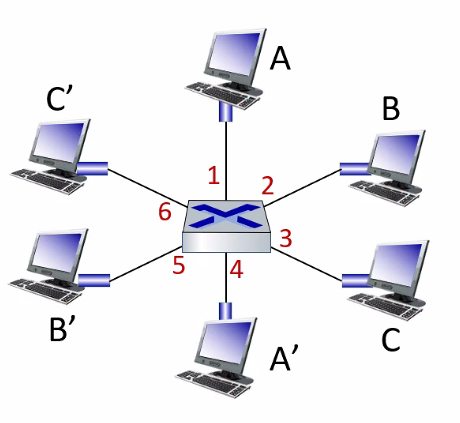
Example: ping some IP address within the network
- your
ARPtable does not contain the MAC of the IP you want to ping- check if by typing
ARP -A
- check if by typing
- do a
ping, and it should work- under the hood
pingdoes theARPfor you
- under the hood
- Now check again your
ARP -A. You should notice that you got an additionalMACaddress from broadcast
Routing to Another Subnet
now let’s look at the more complicated situation when a host on a subnet wants to send a network-layer datagram to a host off the subnet.
Since each adapter are the ones physically receiving packets on each link/egde on the graph, we need to “change” MAC addresses of the packet as otherwise they will be dropped!
Consider the case you want to deliver from 111.111.111.111 to 222.222.222.222
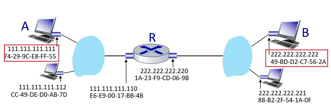
note that routers have MAC addresses, as they are the ones bridging between subnets and possibly the outside world. Also one important point is: link layer treats router and hosts as the same. As their job is to realize the host-router or host-host delivery.
-
First the sender fills out the IP as normal, and the source MAC. We know we need to send to
Rfirst -
So, we want to obtain the MAC address of
Rby usingARPbroadcast (Rwould be the first hop router forA). This can be done since we know the IP for first-hop/default gateway router from DCHP configuration (see Obtaining Host Address: DCHP)- If the sending adapter were to use that MAC address of
222.222.222.222, then none of the adapters on Subnet 1 would bother to pass the IP datagram up to its network layer, since the frame’s destination address would not match the MAC address of any adapter on Subnet 1. Therefore, all the hosts/routers will have dropped the frame (there is only one case that a switch would have dropped. See next section) - to the link-layer, a router = host is indistinguishable. Therefore, without putting
Ras the destination MAC address,Rwould have rejected it and you are done. Hence, this change of MAC address is only when your next hop is a router. (see section Switched Network Example
- If the sending adapter were to use that MAC address of
-
Construct the packet with MAC address of
R, and sends the frame into Subnet 1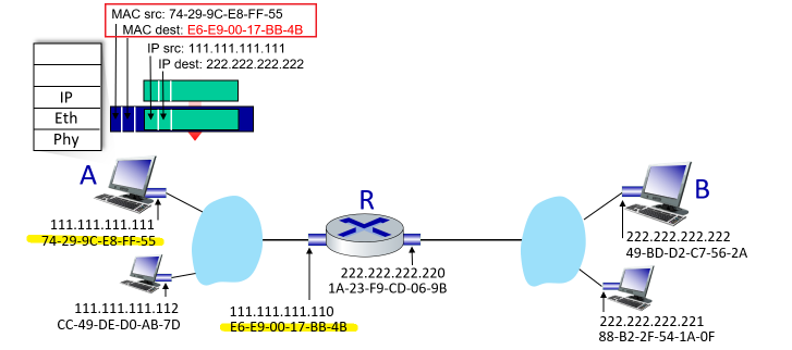
-
Router
Rsees that the link-layer frame is addressed to it, and therefore passes the frame to the network layer of the router -
The router now has to determine the correct interface on which the datagram is to be forwarded, by consulting a forwarding table in the router and the
IP Dest.- The forwarding table tells the router that the datagram is to be forwarded via router interface
222.222.222.220 - now it is related to network layer routing
- The forwarding table tells the router that the datagram is to be forwarded via router interface
-
Router determined the interface, pass it to its adapter. Then, to make sure correct delivery, the MAC addresses are again changed. But what is the MAC address of it’s next hop for
222.222.222.222? -
Use
ARPto determine the MAC address of222.222.222.222, then the packet is finally formed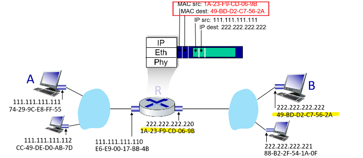
-
The router’s adapter send it to the subnet 2, and
222.222.222.222’s adapter will correctly receive it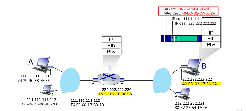
Basically MAC changes is needed to make sure the correct adapters (person) living under the IP (postal address) will take in the frame.
Ethernet
Today, Ethernet is by far the most prevalent wired LAN technology, and it is likely to remain so for the foreseeable future. One might say that Ethernet has been to local area networking what the Internet has been to global networking.
Switched ethernet is more popular today
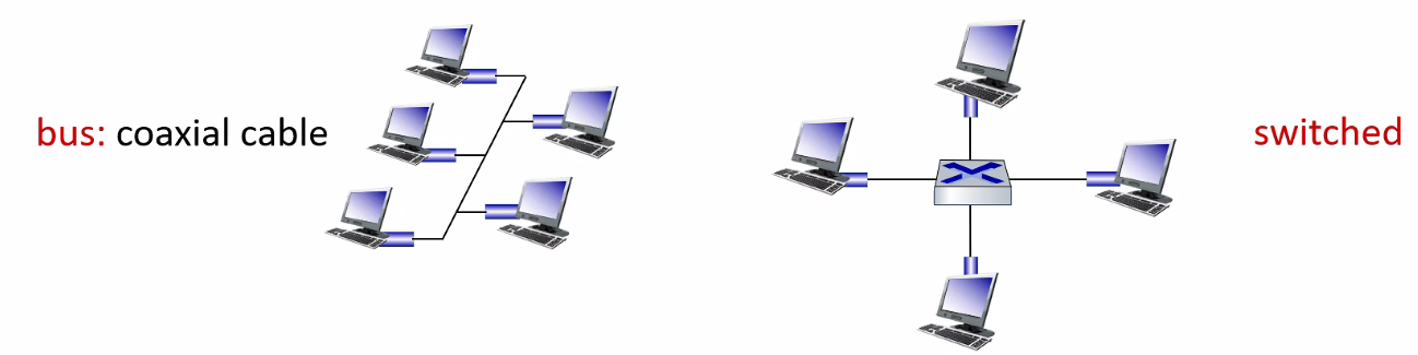
Skipped.
Link-Layer Switches
role of the switch is to receive incoming link-layer frames and forward them onto outgoing links. Some important mechanisms covered here include:
- how a switch figured out what’s the next switch to send to, given a
dst MAC
Note
Again, remember that switch itself is transparent to the hosts and routers in the subnet; that is, a host/router addresses a frame to another host/router (by just filling the IP), and assumes that the transmission is host to router!
- in reality, we know that switches are doing the forwarding and receiving of the frame
Forwarding and Filtering
The two key functions of a switch to operate as we expected is:
- Filtering is the switch function that determines whether a frame should be forwarded to some interface or should just be dropped.
- Forwarding is the switch function that determines the interfaces to which a frame should be directed, and then moves the frame to those interface. If it has no idea, it will flood to all except the incoming port.
Switch filtering and forwarding are done with a switch table. The switch table contains entries for some, but not necessarily all, of the hosts and routers on a LAN.
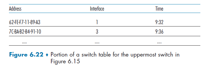
where this idea is indeed similar to a forwarding table of a router.
- But one important distinction is that switches forward packets based on MAC addresses rather than on IP addresses.
To understand how switch filtering and forwarding work, suppose a frame with destination address DD-DD-DD-DD-DD-DD arrives at the switch on interface x. Then the switch indexes its table with the MAC address DD-DD-DD-DD-DD-DD.
- There is no entry in the table for
DD-DD-DD-DD-DD-DD. In this case, the switch forwards copies of the frame to the output buffers preceding all interfaces except for interfacex.- note that unless it is forwarding to a router, it will not change the source MAC address (used for self-learning) capability. An example in Switched Network Example could clarify.
- There is an entry in the table, associating
DD-DD-DD-DD-DD-DDwith interfacex. In this case, the frame is coming from a LAN segment that contains adapterDD-DD-DD-DD-DD-DD. Filter the frame.- this is because it means that
dst DD-DD-DD-DD-DD-DDis broadcasted to it. And since the output interface isx, it means the frame should have already been received by the host withDD-DD-DD-DD-DD-DD - this is the only case that a switch drops a packet intentionally. (recall that a switch has no MAC address)
- this is because it means that
- There is an entry in the table, associating
DD-DD-DD-DD-DD-DDwith interface $y\neq x$. In this case, the frame needs to be forwarded to the LAN segment attached to interfacey.
Example: The situation with upper switch in Figure 6.15.
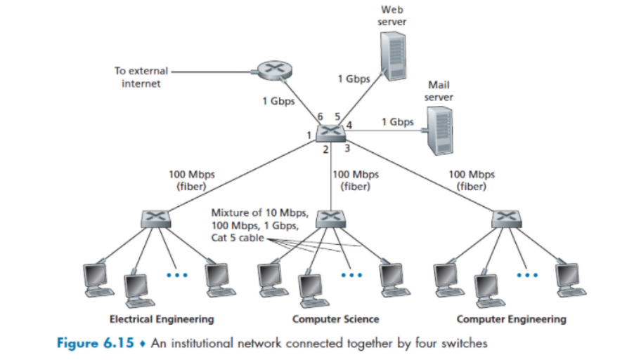
-
Suppose that a frame with destination address
62-FEF7-11-89-A3arrives at the switch from interface1. Suppose we already have the table:then, it sees interface is still
1, so it filters/discards it. (stops the frame to flood to the other subnets!) -
suppose a frame with the same destination address arrives from interface
2. Then it forwards to interface1
It should be clear from this example that as long as the switch table is complete and accurate, the switch forwards frames toward destinations without any broadcasting.
Then, the natural question to ask is how to fill out the forward table?
Self-Learning
Basically it is filled out automatically as there are traffic flowing.
-
The switch table is initially empty.
-
For each incoming frame received on an interface, the switch stores in its table
- the MAC address in the frame’s source address field (if it knows where it comes from, it knows where to send to next time)
- the interface from which the frame arrived
- the current time. (aging time is more like hard-coded)
In this manner, the switch records in its table the LAN segment on which the sender resides. If every host in the LAN eventually sends a frame, then every host will eventually get recorded in the table.
-
The switch deletes an address in the table if no frames are received with that address as the source address after some period of time (the aging time). In this manner, if a PC is replaced by another PC (with a different adapter), the MAC address of the original PC will eventually be purged from the switch table.
Example
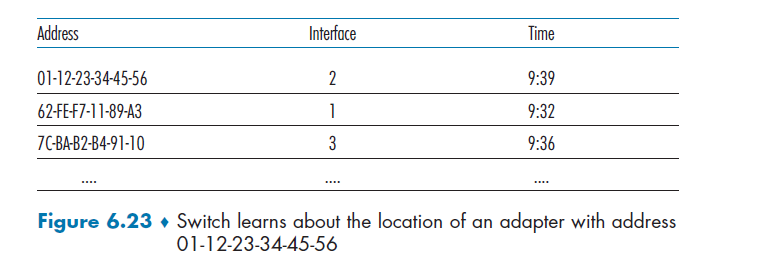
- Suppose at time 9:39 a frame with source address
01-12-23-34-45-56arrives from interface 2. Suppose that this address is not in the switch table. Then the switch adds a new entry to the table, as shown in Figure 6.23 - suppose that the aging time for this switch is 60 minutes, and no frames with source address
62-FE-F7-11-89-A3arrive to the switch between 9:32 and 10:32. Then at time 10:32, the switch removes this address from its table.
Properties of Switches
One key difference of switches against multiaccess medium is that:
- Elimination of collisions. In a LAN built from switches (and without hubs), there is no wasted bandwidth due to collisions, since we have dedicated buffers/links, everything is in order.
- Heterogeneous links. Because a switch isolates one link from another, the different links in the LAN can operate at different speeds and can run over different media.
- Management. In addition to providing enhanced security (see sidebar on Focus on Security), a switch also eases network management. For example, if an adapter malfunctions and continually sends Ethernet frames (called a jabbering adapter), a switch can detect the problem and internally disconnect the malfunctioning adapter.
Switched Network Example
Here we demonstrate an example of delivering from Host A to Host B through two switches in the same network.
Resource
- animation is from https://www.practicalnetworking.net/stand-alone/communication-through-multiple-switches/
Consider the following setup
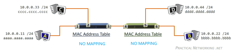
and suppose Host A already know the MAC address of Host B
- if it didn’t, then host
Awill send outFF-FF-FF-FFARP broadcast and flood all the way to hostB. During that process, the learning of mapping in switches will happen in the same manner as below - but regardless, to begin, the MAC address tables for both switches will be empty.
Then, to send from A to B:
-
Sender
Acomposes a frame with destination IP and MAC filled to beBB-BB-BB-BB, and send to the blue switch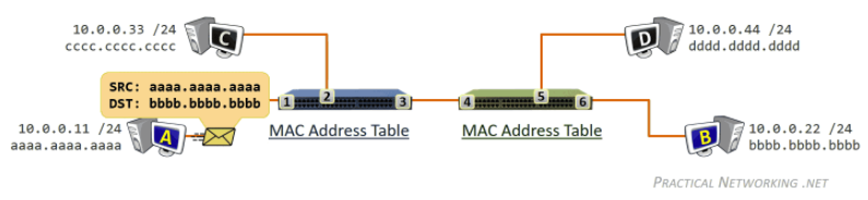
-
frame arrives on the blue switch. Empty MAC table, so blue switch learns the MAC address
aaaa.aaaa.aaaaexists on port1.
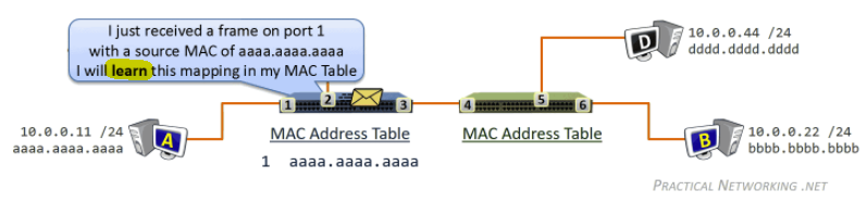
-
since the blue switch does not yet have an entry in his MAC address table for
bbbb.bbbb.bbbb, the frame is duplicated and flooded out every port (notice we do not change `src/dst` MAC like the case with router, as only router changes that)Flooding Filtering 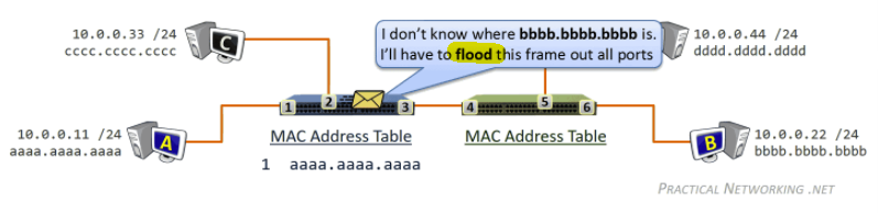
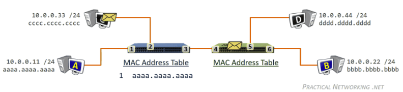
where due to filtering Host
Cwill reject/discard the packet -
The frame will also arrive on the green switch. Just like the other switch, the first thing the green switch will do is learn that it received a frame on port
4with a source MAC address ofaaaa.aaaa.aaaa.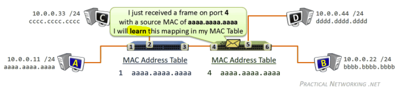
-
Just like the other switch, the green switch does not know where the MAC address
bbbb.bbbb.bbbbexists, so the frame will again be duplicated and flood out each switch port.Flooding Filtering 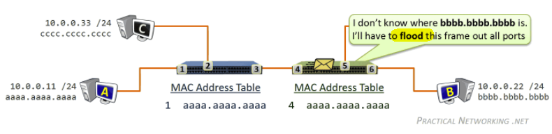
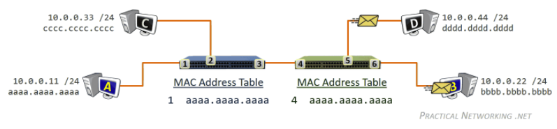
-
Delivered and Mapping learnt!
Now, for reply, host B want to reply to host A. This time it is easier as we already learned the mapping to aaaa.aaaa.aaaa.aaaa
-
In the response frame sent by Host B to Host A, the Layer2 header will have a Source MAC address of
bbbb.bbbb.bbbband a Destination MAC address ofaaaa.aaaa.aaaa. Then hostBsends to the green switch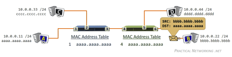
-
The response frame will first arrive on the green switch on port
6. Therefore, the green switch will learn that the MAC addressbbbb.bbbb.bbbbexists out port6.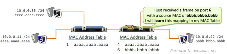
-
green switch then consults its MAC address table to determine that the frame destined to
aaaa.aaaa.aaaashould be forwarded out port4. (notice how we don’t have flooding now, since we know where to send!)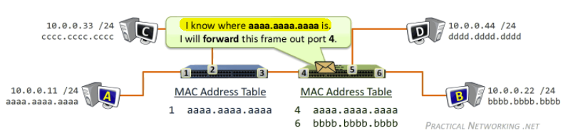
-
blue switch will learn the MAC address
bbbb.bbbb.bbbbexists out port3.
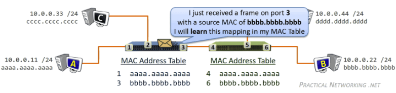
-
blue switch then consults its MAC address table to determine that the frame destined to
aaaa.aaa.aaaashould be forwarded out to port1. (again, no need to flood!)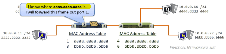
-
Host
Areceived the packet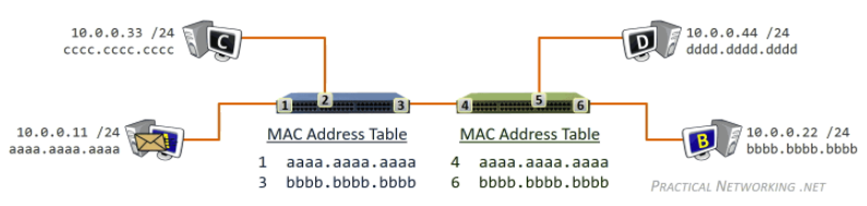
Notice that:
- the backward trip will be easier than the forward trip as routers will have learned the
src_MAC - after two messages (one round trip), both routers have learned both the mappings fully!
VLANS
Consider the following case
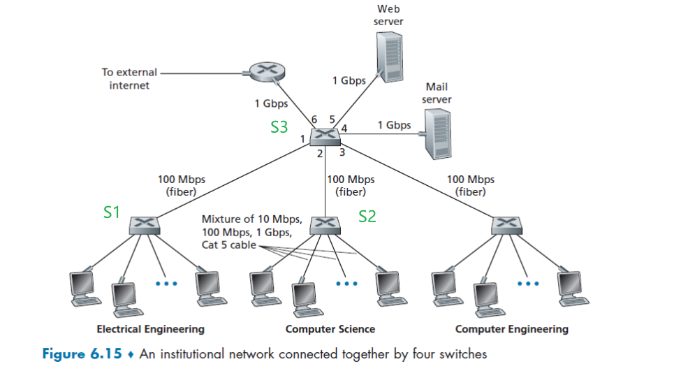
But now, we would like to solve the following problem:
- traffic isolation: broadcast traffic (e.g., frames carrying ARP and DHCP messages or frames whose destination has not yet been learned by a self-learning switch) must still traverse the entire institutional network, and we don't want that so we can:
- improve LAN performance as we have less traffic
- provide security/isolation between departments so packets don’t freely go anywhere
- Inefficient use of switches: what if we have 10 departments but we don’t want to use 10 switches?
- Managing users. If an employee moves between groups, the physical cabling must be changed to connect the employee to a different switch in Figure 6.15. Employees belonging to two groups make the problem even harder
Whereas the first problem technically can be solved by replacing the central switch S3 with 6 ports to be a router, such that:
-
if an EE laptop wants to talk to CS laptop, and suppose they know the IPs, then:
- Link Layer broadcast will only aims to obtain the MAC of router
R3=S3 - Packet sent to that router
R3 - Router sends out to port 2 due to OSPF, switch
S2receives it - Switch
S2broadcast to know the MAC of that CS laptop - Switch delivers the packet with filled in MAC addresses to the CS laptop
so we see that in the end, broadcast never crossed from CS to EE, and we can still talk to each other
- Link Layer broadcast will only aims to obtain the MAC of router
However, this does not solve the second and third problem. So in general, the solutions is to use VLAN (virtual local area network)+ embedded router.
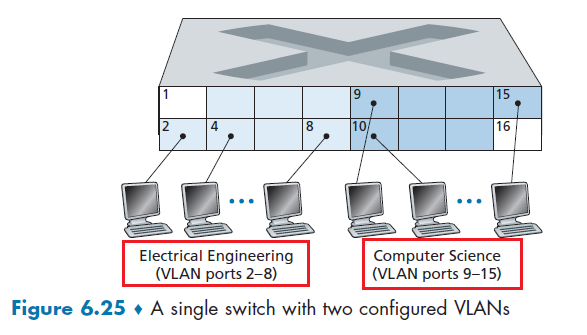
where in a single switch
- the switch’s ports (interfaces) are divided into groups by the network manager, and each group constitutes a VLAN, with the ports in each VLAN forming a broadcast domain
- therefore, hosts within a VLAN communicate with each other as if they (and no other hosts) were connected to the switch
- now, if we stop here, CS and EE are isolated since broadcast can never reach across as they are in the same switch. But this also means they cannot talk to each other at all.
- connect a VLAN switch port (e.g., port 1 in Figure 6.25) to an external router and configure that port (e.g. port 1) to belong both the EE and CS VLANs. This is usually done internal by a device that contains both VLAN and router (built by the vendor)
- in the end, both router and switch does the task of: given packet, forward to a port. The difference is what is inside the forwarding table. So this is certainly doable to make such a product.
The upshot of what we are doing is so that:
- physical configuration looks like EE and CS departments share the same physical switch
- gives isolation
- shares/saves switches
- logical configuration would look as if the EE and CS departments had separate switches connected via a router.
- An IP datagram going from the EE to the CS department would first cross the EE VLAN to reach the router and then be forwarded by the router back over the CS VLAN to the CS host.
- again, isolation and communication would both work.
Now, this is up and working. Often there comes another requirement that people in the same department lives in different buildings. Therefore, you cannot just have a single switch to do VLAN.
Then, you come up with two solutions:
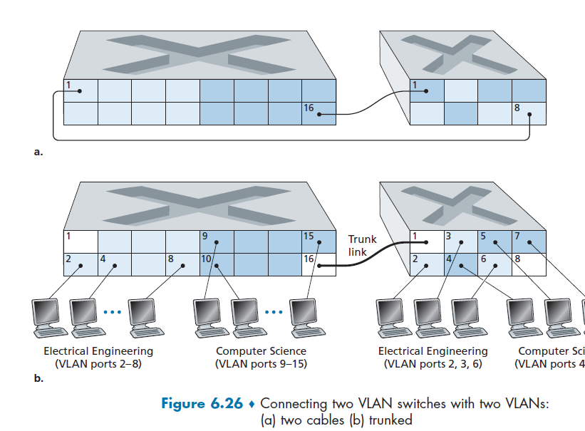
- solution A: for each VLAN group, use a cable to connect them. This means if you have $N$ VLAN groups and two switches, you need $2N$ ports dedicates to do just that. Hence this doesn’t scale!
- solution B: VLAN trunking. A special port on each switch (port 16 on the left switch and port 1 on the right switch) is configured as a trunk port to interconnect the two VLAN switches by belonging to ALL VLAN.
- this means that, if you want to send to (any) the EE VLAN, port 16 will also forward it to switch on the right, but also added a tag to tell the the trunk link on the other side which VLAN this is aimed at (i.e. VLAN EE)
- this adding of tag is the extended Ethernet frame format, 802.1Q, for frames crossing VLAN trunk
The extended ethernet frame therefore looks like this:
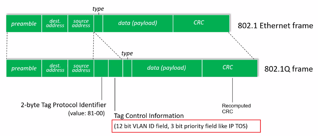
where it is specifically used for VLAN trunking:
- VLAN tag is added into a frame by the switch at the sending side of a VLAN trunk
- then, parsed, and removed by the switch at the receiving side of the trunk.
Therefore, in for every VLAN switch, we need two special/reserved ports:
- port for “routing” in between VLANS (e.g. port 1)
- port for trunking (e.g. port 16)
Data Center Networking
Broadly speaking, data centers serve three purposes.
- First, they provide content such as Web pages, search results, e-mail, or streaming video to users.
- therefore, latency is the single most important metric!
- Second, they serve as massively-parallel computing infrastructures for specific data processing tasks, such as distributed index computations for search engines.
- Third, they provide cloud computing to other companies.
- so 2 and 3 combined also means you need thousands of hosts/servers running.
Therefore, the networking evolved to be some interesting architecture
Data Center Architectures
The worker bees in a data center are the hosts. The hosts in data centers, called blades and resembling pizza boxes, are generally commodity hosts that include CPU, memory, and disk storage.
-
So, it looks like this.
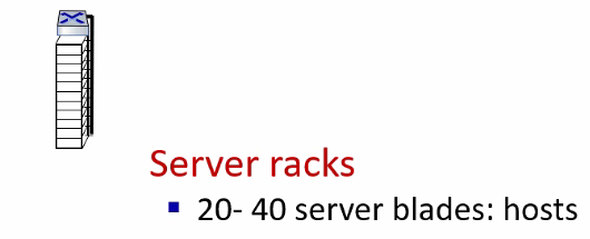
where
-
hosts are stacked in racks, with each rack typically having 20 to 40 blades.
-
At the top of each rack, there is a switch, aptly named the Top of Rack (TOR) switch, that interconnects the hosts in the rack with each other and with other switches in the data center
-
Then, remember that we need to eventually deal with connections in between hosts. So we also need switches that interconnect the TOR switches:
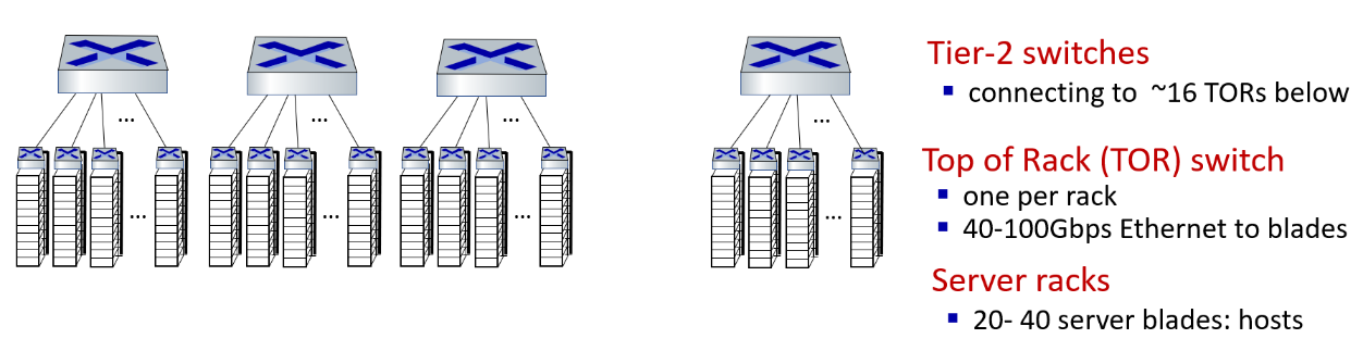
Then, since there are lot of them, we need another layer
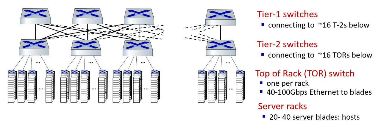
where:
- we basically have a fully connected graph for the T2 Switch and T1 switch, so we can ensure traffic inside can go to anywhere
Finally since he data center network supports two types of traffic:
- traffic flowing between external clients and internal hosts
- traffic flowing between internal hosts
We finish the topology by putting border routers which can connect to the outer world
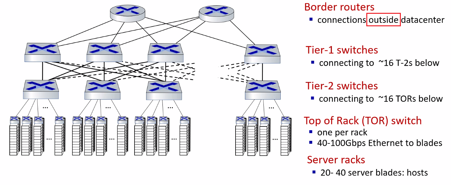
notice that:
- only the very top layer has router.
- all the layers below uses switches for faster communication
Load Balancing in Data Centers
Often we also have load balancer servers in the network so we can sustain the millions of request coming everyday
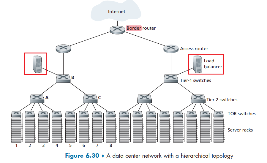
where obviously the job of load balancer is to simply decide and forward requests/traffic so that the load is balanced in your network.
- now all the requests are centralized to load balancer, but that’s ok since you can easily duplicate/scale them as they only performs simple, stateless tasks!
Therefore, when a request comes, this happens:
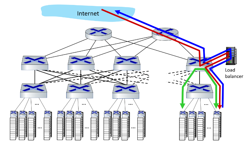
- the load balancer forwards it to one of the hosts that handles the application. (red line)
- this means if need to map the external IP to some internal IP for work
- A host may then invoke the services of other hosts to help process the request. (green line)
- results sent back to load balancer (the only one who knows external/client IP), which is then replied back (blue line)
- translate the internal IP back to the target external IP
Notice
The load balancer not only balances the work load across hosts, but also provides a NAT-like function:
- translating the public external IP address to the internal IP address of the appropriate host
- then translating back for packets traveling in the reverse direction back to the clients.
Hierarchical structure in Real life
In real life, a bit more is happening that the figure below:
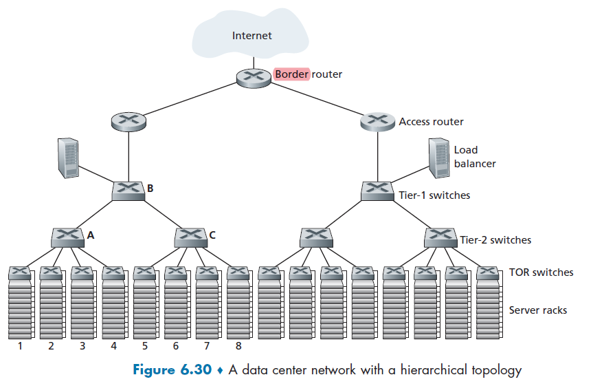
where:
-
some network components are duplicated for doing redundant work, so high availability is ensured
- the hosts below each access router form a single subnet. In order to localize ARP broadcast traffic, each of these subnets is further partitioned into smaller VLAN subnets
- there are more than 1 connection link between a TOR and a switch, and a T1 switch with T2 switch (below discusses why)
Multiple Routes
Consider the setup of, in Figure 6.30:
- each host connects to its TOR switch with a 10 Gbps link
- links between switches are 100 Bbps
Then this means two hosts in the same rack can always communicate at a full 10 Gbps. But what if we have 40 simultaneous flows between 40!pairs of hosts in different racks.
- e.g. each of 10 hosts in rack 1 in Figure 6.30 sends a flow to a corresponding host in rack 5. then rack 2 to rack 6, rack 3 to rack 7, and finally rack 4 to rack 8.
- notice that all racks 1-4 above are in the same Tier 2 switch!
If each flow evenly shares a link’s capacity with other flows traversing that link, then the 40 flows crossing the 100 Gbps A-to-B link (as well as the 100 Gbps B-to-C link) will each only receive:
\[100 \text{ Gbps } / 40 = 2.5 \text{ Gbps }\]which is less than 10 Gbps of the TOR link can handle at max.
There are many solutions, but the common one used is to provide multiple path by increase connectivity in the graph
- e.g. each TOR switch could be connected to two tier-2 switches, which then provide for multiple link- and switch-disjoint paths between racks
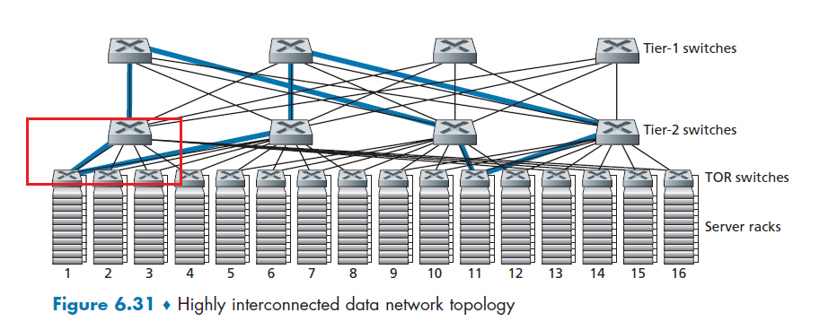
Therefore, now you have:
- four distinct paths between the first tier-2 switch and the second tier-2 switch, together providing an aggregate capacity of 400 Gbps between the first two tier-2 switches
Take-away message
Therefore, one key difference between routing inside data centers and Internet is that:
- instead of choosing between them (like routers in routing), you use all of them.
- you want to have multipath routing being the default standard!
Datacenter Networks: Protocol Innovations
Usually, to transfer things between host, we needed to form packets. send across, receive, and etc.
Again, since latency is critical, congestion control protocols such as TCP and its variants do not scale well in data centers.
Therefore:
- link layer:
- RoCE: remote DMA (RDMA) over Converged Ethernet. This can
- directly read/write into memory in remote hosts
- gives a huge saving to CPUs
- RoCE: remote DMA (RDMA) over Converged Ethernet. This can
- transport layer:
- ECN (explicit congestion notification) used in transport-layer congestion control (DCTCP, DCQCN).
- We use ECN because we cannot afford using
timeout/packet drops as loss event, which will cause a large loss of capacity even if it is just a few seconds. - latency/performance is the biggest thing in datacenter networks
- We use ECN because we cannot afford using
- experimentation with hop-by-hop (backpressure) congestion control
- ECN (explicit congestion notification) used in transport-layer congestion control (DCTCP, DCQCN).
- routing, management:
- SDN widely used within/among organizations’ datacenters
- place related services, data as close as possible (e.g., in same rack or nearby rack) to minimize tier-2, tier-1 communication
- e.g. MAP-reduce: doing computations for servers that are close to each other
A Day in Life of Web Page Request
our journey down the protocol stack is now complete!
-
application, transport, network, link
-
putting-it-all-together: synthesis!
Suppose you want to do something on google, and you sent a request
-
Suppose your laptop on campus does it. First, when your Laptop connects, you need DHCP to give you IPs!
-
DCHP request inside UDP segment, and then inside IP datagram with a broadcast IP destination address (
255.255.255.255) and a source IP address of0.0.0.0 -
Gets into a frame, and the destination will be
FF-FF-FF-FFso hopefully it will reach the DHCP server. The frame’s source MAC address is that of Bob’s laptop,00:16:D3:23:68:8A -
switch broadcasts the incoming frame on all outgoing ports, including the port connected to the router.
-
The router receives the broadcast Ethernet frame containing the DHCP request on its interface (with MAC address
00:22:6B:45:1F:1B). The datagram’s broadcast IP destination address indicates that this IP datagram should be processed by upper layer protocols at this node, so the datagram’s payload (a UDP segment) is thus demultiplexed (Section 3.2) up to UDP, and the DHCP request message is extracted from the UDP segment. -
Suppose DHCP server allocates address
68.85.2.101to Bob’s laptop. Then DHCP server creates a DHCP ACK message (Section 4.3.3) containing this IP address, as well as- the IP address of the DNS server (68.87.71.226)
- the IP address for the default gateway router (68.85.2.1)
- the subnet block (68.85.2.0/24) (equivalently, the “network mask”).
The Ethernet frame has a source MAC address of the router’s interface to the home network (
00:22:6B:45:1F:1B) and a destination MAC address of Bob’s laptop (00:16:D3:23:68:8A). -
Ethernet frame containing the DHCP ACK is sent (unicast) by the router to the switch. Because the switch is self-learning (Section 6.4.3) and previously received an Ethernet frame (containing the DHCP request) from Bob’s laptop, the switch knows to forward a frame addressed to
00:16:D3:23:68:8Aonly to the output port leading to Bob’s laptop. -
Bob’s DHCP client then records its IP address and the IP address of its DNS server. It also installs the address of the default gateway into its IP forwarding table (Section 4.1). Bob’s laptop will send all datagrams with destination address outside of its subnet `68.85.2.0/24` to the default gateway
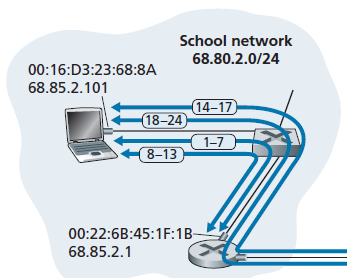
-
-
Then, when Bob types the URL for www.google.com into his Web browser. To in the end connect to the server with a TCP socket, we we want to do DNS query to find out the IP address first
- The operating system on Bob’s laptop thus creates a DNS query message, putting the string “www.google.com” in the question section of the DNS message. This is then packed into a UDP, and then an IP packet with
- an IP destination address of
68.87.71.226(the address of the (not local) DNS server returned in the DHCP ACK above) - a source IP address of
68.85.2.101.
- an IP destination address of
- Since the IP is outside the subnet, it will be first sent to the gateway router in Bob’s school’s network. However, though we know the IP of that, we don’t know the gateway router’s MAC address. In order to obtain the MAC address of the gateway router, Bob’s laptop will need to use the ARP protocol
- Bob’s laptop creates an ARP query message with a target IP address of
68.85.2.1(the default gateway), places the ARP message within an Ethernet frame with a broadcast destination address (FF:FF:FF:FF:FF:FF) and sends/floods the Ethernet frame to the switch - All connected devices, including the gateway router received the Link Broadcast. The gateway router finds that the target IP address of
68.85.2.1in the ARP message matches the IP address of its interface. Then:- The gateway router thus prepares an ARP reply, indicating that its MAC address of
00:22:6B:45:1F:1B - It places the ARP reply message in an Ethernet frame, with a destination address of
00:16:D3:23:68:8A(Bob’s laptop) and sends the frame to the switch
- The gateway router thus prepares an ARP reply, indicating that its MAC address of
- Bob’s laptop receives the frame containing the ARP reply message and extracts the MAC address of the gateway router (
00:22:6B:45:1F:1B) from the ARP reply message. - Bob’s laptop can now (finally!) address the Ethernet frame containing the DNS query to the gateway router’s MAC address.
- Note that the IP datagram in this frame has an IP destination address of
68.87.71.226(the DNS server), while the frame has a MAC destination address of00:22:6B:45:1F:1B(the gateway router).
- Note that the IP datagram in this frame has an IP destination address of
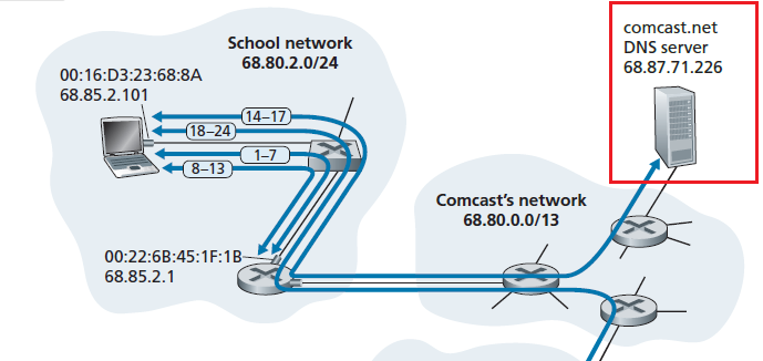
- The operating system on Bob’s laptop thus creates a DNS query message, putting the string “www.google.com” in the question section of the DNS message. This is then packed into a UDP, and then an IP packet with
-
Finally, Bob can send the DNS query with the packet information complete. Now we need to route the packet
- The gateway router first receives the frame and extracts the IP datagram containing the DNS query. The router looks up the destination address of this datagram (
68.87.71.226) and determines from its forwarding table that the datagram should be sent to the leftmost router in the Comcast network- eBGP tells the gateway and passed information throughout the internal AS reachability of IP such as Comcast’s network.
- iBGP tells each router inside the network which gateway router to go to depending on which AS I want to go to. This will be used if the first-hop router is not the gateway router.
- then the route to that gateway is done by OSPF
- leftmost router in the Comcast network receives the frame, extracts the IP datagram, examines the datagram’s destination address (
68.87.71.226)- look at its own forwarding table, which has been filled in with intra-domain protocol (such as RIP, OSPF or IS-IS)
- determines the outgoing interface
- Eventually the IP datagram containing the DNS query arrives at the DNS server. Then:
- looks up the name www.google.com in its DNS database, and finds the DNS resource record that contains the IP address (
64.233.169.105) for www.google.com - if this doesn’t have it, we will need to do the query to authoritative DNS server or TLD server, and etc.
- forms a DNS reply message containing this hostname-to-IP address mapping, and places the DNS reply message in a UDP segment to get back to Bob
- looks up the name www.google.com in its DNS database, and finds the DNS resource record that contains the IP address (
- Bob’s laptop extracts the IP address of the server www.google.com from the DNS message. Finally, after a lot of work, Bob’s laptop is now ready to contact the www.google.com server
- The gateway router first receives the frame and extracts the IP datagram containing the DNS query. The router looks up the destination address of this datagram (
-
Then, you got a DNS reply and has an IP for google.com. Now you establish the TCP connection to that IP.
-
create the TCP socket (Section 2.7) that will be used to send the HTTP GET message (Section 2.2.3) to www.google.com
- route all the way to google’s IP
- perform a three-way handshake (Section 3.5.6) with the TCP in www.google.com
- essentially TCP segment inside an IP datagram with a destination IP address of
64.233.169.105(www.google.com), places the datagram inside a frame with a destination MAC address of00:22:6B:45:1F:1B(the gateway router) and sends the frame to the switch.
-
routers in the school network, Comcast’s network, and Google’s network forward the datagram containing the TCP SYN toward www.google.com, using the forwarding table in each router
- includes both intra-domain protocol such as OSPF and inter-domain routing such as GBP
-
the datagram containing the TCP SYN arrives at www.google.com.
- The TCP SYN message is extracted from the datagram and demultiplexed to the welcome socket associated with port 80.
- A connection socket is created for the TCP connection between the Google HTTP server and Bob’s laptop.
- TCP
SYNACKis sent back to Bob’s laptop (routes all the way back)
-
(some steps skipped for three-way handhshake)
-
With the socket on Bob’s laptop now (finally!) ready to send bytes to www.google.com, Bob’s browser creates the HTTP
GETmessage (Section 2.2.3) containing the URL to be fetched.- HTTP
GETmessage is then written into the socket, with theGETmessage becoming the payload of a TCP segment. - The segment is placed in a datagram and delivered all the way alike step 1 - 3 mentioned above
- HTTP
-
Google does the same thing to respond
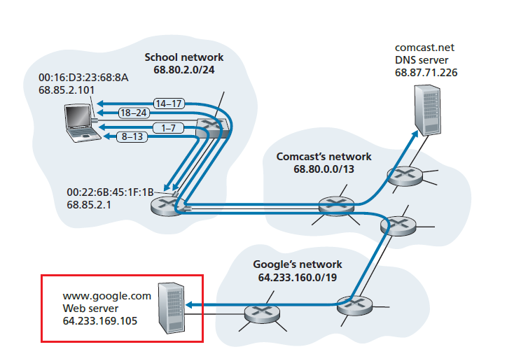
-
This completes the entire tour!
Miscellaneous
Useful stuff learnt throughout the semester
Wireshark
The basic structure of this is:
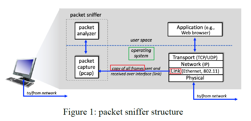
where the packet sniffer, is shown within the dashed rectangle in Figure 1
First, we have the capturing:
- the actual capturing is the COPYING of Link Layer Frames which happesn in the Kernel Space
- messages exchanged by higher layer protocols such as HTTP, FTP, TCP, UDP, DNS, or IP all are eventually encapsulated in link-layer frames that are transmitted over physical media
Then, we have the analysis to displays the contents of all fields within a protocol message
-
In order to do so, the packet analyzer must “understand” the structure of all messages exchanged by protocols
For example, it needs to:
- understand the format of Ethernet frames, and so can identify the IP datagram within an Ethernet frame.
- It also understands the IP datagram format, so that it can extract the TCP segment within the IP datagram.
- Then, it understands the TCP segment structure, so it can extract the HTTP message contained in the TCP segment.
- Finally, it understands the HTTP protocol and so, for example, knows that the first bytes of an HTTP message will contain the string “GET,” “POST,” or “HEAD,” as shown in Figure 2.8 in the text.
Technically speaking, Wireshark is a packet analyzer that uses a packet capture library in your computer
Intro to Wireshark
After you select which network interface (网卡) to capture, you will see stuff like this:
-
if you clicked the wrong one accidentally, you can change it here:
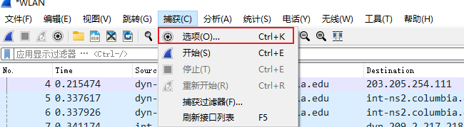
Then, your screen looks like this
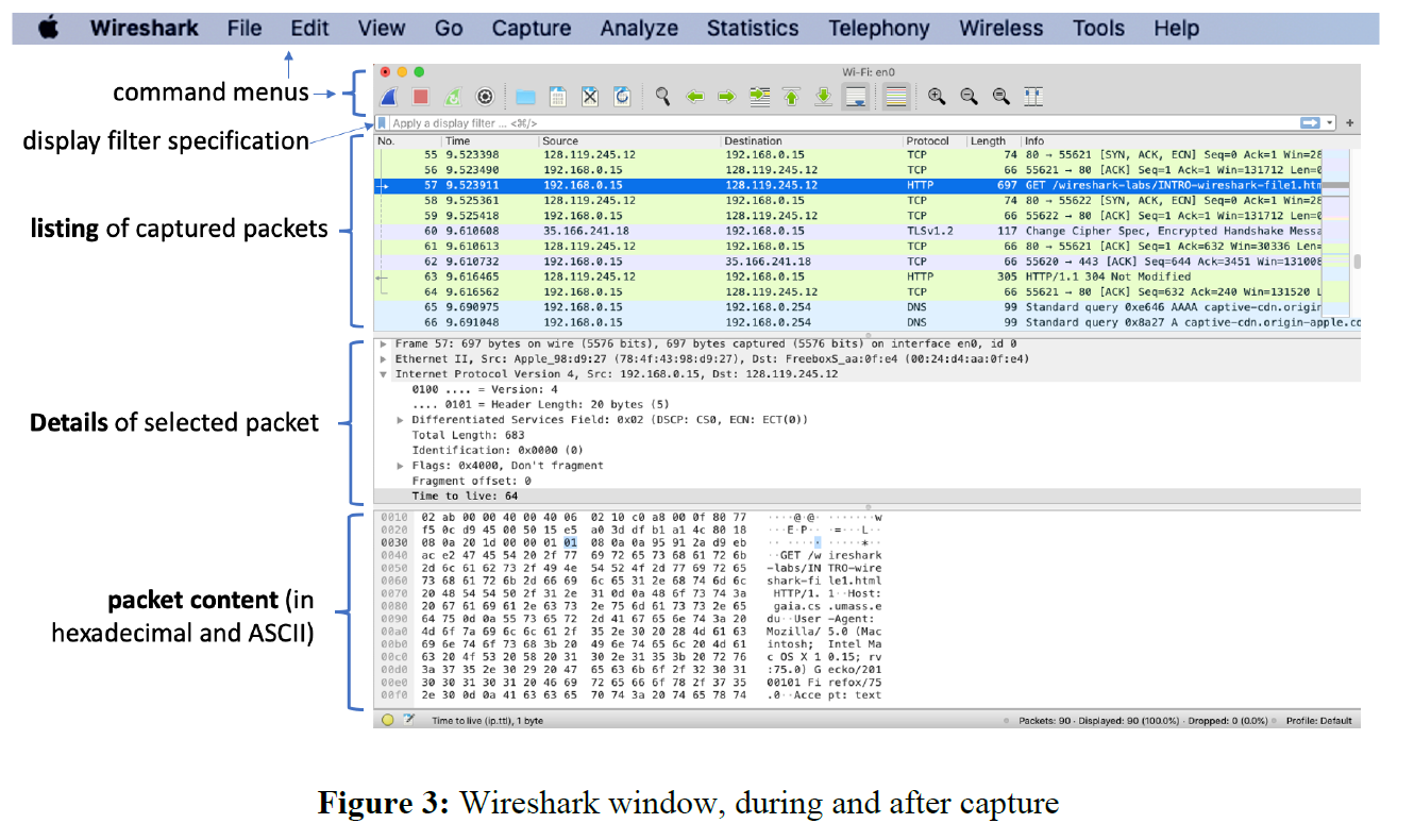
where basically:
- packet content contains entire contents of the captured frame in ASCII and hexadecimal without parsing
- packet details contains the parsed contents
The rest is basic and you know already.
Distributed Hash Tables
Recall that it is useful when you have P2P, we are centralizing all the information, which might be bad for load balance or availability.
Here, we consider having a distributed node for maintaining the information as a solution.
The simplest idea:
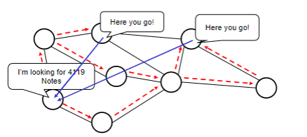
where if you do a exhaustive search, then if only $K$ out of $N$ nodes have the information, your expected search cost is at least $N/K$ searches, which is $O(N)$.
Therefore, the aim is to minimize the search cost using distributed search table.
Heuristics
This is slow because we are doing some exhausted search. So we want to speed up by having a more directed search
- assign particular nodes to hold particular content (or know where it is, like an information booth)
- when a node wants that content, go to the node directly that is supposed to have or know about it
DHT Step 1: The Hash
First we need to design a hash function $h$, that hashes the content being searched for to a identifier.
\[h(\text{"movie xxx"}) = 8045\]Then distribute that range of hash function (responsibility) among all nodes.
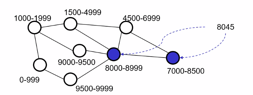
note that multiple nodes can hold the same content ofc.
- one problem still remains is how to figure out where to go when we have the hash
DHT Step 2: Routing
Now we need to find a way to reach the object when we have the hash. Obviously we want to achieve that:
- For each object, node(s) whose range(s) cover that object (i.e. is responsible for it) must be reachable via a “short” path
- number of neighbors for each node should not go $O(N)$, otherwise its like a centralized system.
In essence, the different approaches (CAN,Chord,Pastry,Tapestry) differ fundamentally only in the routing approach
Case Studies
Here we cover In alphabetical order:
- CAN (Content Addressable Network)
- Chord
In particular, consider the questions:
- How is hash space divided “evenly” among existing nodes?
- How is routing implemented that connects an arbitrary node to the node responsible for a given object?
- How is the hash space repartitioned when nodes join/leave? (i.e. how is the structure changing)
For the following discussion:
- Let $N$ be the number of nodes in the overlay
- $H$ be the size of the range of the hash function (when applicable)
CAN
Every content/object maps to a point in this cartesian space. We decide on a dimension $D$ that we want to have. Here, let us take $D=2$. Therefore, we basically have:
- hash value for each point in the space
- each node is responsible for a volume of hash value/points in the space
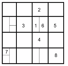
where basically:
-
**every square is occupied by Some numbers are not labelled for clarity purposes.
- you are directedly connect to your neighbor, which is defined to be the cube that is touching your cube. Therefore, there is only $O(D)$ neighbors.
- this is assumed to be wrapped around, so node $7$ and $8$ are neighbors.
- in this setup, we can figure out the path geometrically
CAN Routing
The upshot is that each coordinate on the map is related to the hash value of the object. Therefore, each node/square on the diagram knows exactly where to look at.
Consider in this case that 1 wants to get the information X which is in the lower half of node 8.
- compute the cartesian distance to the data
X. In this case, the route through2is the shortest due to the wrap around. - therefore, since
node 1can only contact its neighbor, it send it tonode 2. - this happens iteratively until it reaches
node 8.
CAN Node Insertion
Basically when you have a new node:
- find some node in the CAN network
- choose a point in that space uniformly at random
- using CAN, inform the node that currently covers the space (because you are going to take some responsibility from it soon)
- the node will then split its space into half by dimension (i.e. along some axis)
So basically every new node will take half of the space of some existing node. This can therefore achieve load balancing, since for node with high responsibility = large area = high probability of being shared when a node joined.
CAN Removal Process
Basically like balancing a tree. In general, there are two situations:
-
You can simply collpase the removed node’s portion to form a bigger rectangle
- e.g. if 6 is removed, then its portion is given back to 1
-
The node is the only one in the rectangle. Then you need juxtaposition
-
e.g. if 3 is removed, then it should merge the space back to node 2,4,5. One way is to let 5 take over that space, while node 2 take over node 5’s previous space
-
basically it looks like balancing a tree
|
 |
| 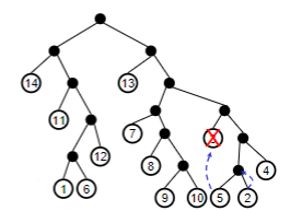 |
| :———————————————————-: | :———————————————————-: |
|
| :———————————————————-: | :———————————————————-: |so the algorithm basically becomes the follows. Suppose node
sis leaving:-
Find a leaf node
tthat is either-
s’s sibling (i.e. in the first case mentioned above) -
descendant of
s’s sibling wheret’s sibling is also a leaf node (i.e. the second case mentioned above)- in this case, if
sis node 6, thentis either node 2 or 5. Node 4 does not work since its sibling is not a leaf.
- in this case, if
-
-
Found
t, then letttake overs’s space -
t’s sibling then take over thet’s previous space
-
-
Chord
The only difference here is basically we are having nodes all in a 1-dimensional space. Therefore, instead of hashes that gives some d-dimensional coordinate, this gives a one dimensional ID.
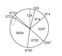
where the chord is basically wrapped around to form a circle.
Hence Chord Basically works as follows
- hash the IP address of a node
- each node covers object/data from previous hashed ID up to its own
- therefore, the hash of object itself tells you where to look for the node
Chord Routing
First we need decide the “neighbors each node knows”. In this case, each node knows several other nodes beside its immediate neighbor (in contrast to CAN).
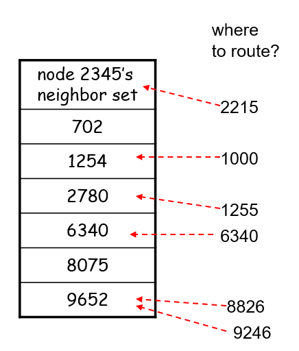
where here, we are node 2345, and we:
- know 6 other nodes’ ID
- then if we need data with hash of
1000, we will ask node1254(since each node covers object from previous ID up to its own)
in terms of implementation, the finger table needs to be ordered clockwise. (most often)
Implementation
Let the range of the hash function be $H$ (i.e. the length of the chord is $H$). Then, we can define:
-
A node
\[t + \text{mod}_H(2^i )\]t’s neighbor as the closest node to:for some $i$. Basically this ensures that there is at most $\log_2 H \to \log_2 N$ neighbors, since we only have $N$ nodes in the chord. (In contrast to CAN, which is independent of $N$).
-
notice that the length of the chord between two nodes is proportional to the probability of being picked when a new node inserts. This basically achieves load balancing.
For instance, if you are node 67, iterating all the i’s gives you:
| 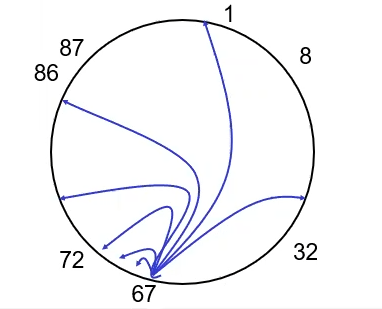 |
| 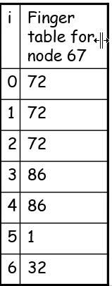 |
| :———————————————————-: | :———————————————————-: |
|
| :———————————————————-: | :———————————————————-: |
where here we took $H=100$, then:
- the blue lines are the computed neighbor
- the black numbers are the actual neighbors (i.e. closest to the computed one)
- the table on the right are the values
Chord Node Insertion
Suppose we are adding node 82 into the system.
-
First we need find the
82’s predecessor, which is basically node72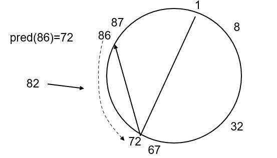
-
Then, we can set the finger table for node
82by computing from node `72` (i.e. let node72compute the data and put it in node82):
where basically:
- the value $t + \text{mod}_H(2^i )$ is computed from node
82 - the lookup for closest node from that value is done by node
72
- the value $t + \text{mod}_H(2^i )$ is computed from node
-
Next, we need to update the finger table of other nodes who should now contain entries to `82`. This can be done by:
-
Go to the largest node before or at ID $82 - 2^i$, and let us call that node
t.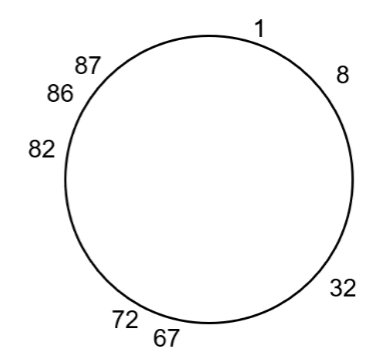
e.g., for $i=1$, we will reach node
72, which we know should update its finger table. -
If node
t’s $2^i$ finger points to a node larger than $82$:-
change that pointer to $82$
-
set node
tto its current predecessor, and repeat step 2e.g. for $i=3$, we will need to update the red highlighted nodes:
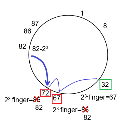
where basically:
- we first jumped to node
72and change the $2^3$ finger of node72to now point to node82instead of86 - go to
72’s predecessor and do the same, for its $2^3$ finger - go to
32, and realize that we need no update. Hence we terminate here for $i=3$.
- we first jumped to node
Else, move on to the next $i$ value
-
-
Repeat for all the $i$ values.
- therefore, in total it takes $O(\log^2N)$ time to find and update all.
-
Chord Node Deletion
The idea is basically the same as insertion, where suppose node 82 is to be deleted, then we need to replace the finger table with node 86 instead:
-
Find node
82’s successor, which is node86 -
Perform step 3 in the Chord Node Insertion, basically undoing it for node `82`
e.g. if we are at $i=3$ now, then we compute $82-2^3$
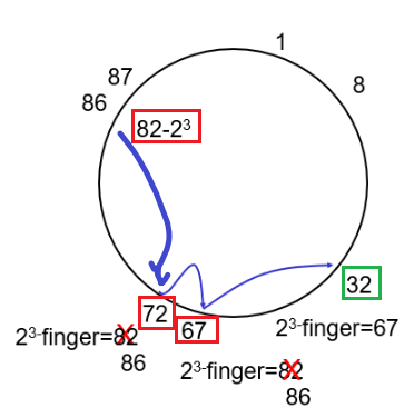
where notice that we are computing $82-2^3$ at node `86`:
- first jumped to node
72and change the finger back to node86if it was pointing to node82 - etc.
- first jumped to node
Using newudpl
This section includes details on how to use and debug newudpl from http://www.cs.columbia.edu/~hgs/research/projects/newudpl/newudpl-1.4/newudpl.html
The mechanism seems as follows. If you run:
➜ ./newudpl -i 127.0.0.1:41192 -s50 -d2.004 -v
Then it will:
- only accept packets from
-i 127.0.0.1:*, and listens on the default address127.0.0.1:41192(so your client needs to send there) - and it redirects packet out to the default address
127.0.0.1:41194(so your server needs to listen here)
Then, what you then do is to:
-
let python
clientto send data to41192, assuming it is using some portsender_port➜ python tcpclient.py Input: aaa yeet # recevied from server after step 2 -
let python
serverto receive data from41194, and reply directly tosender_portof the client➜ python tcpserver.py The server is ready to s ss receive [LOG] servicing ('127.0.0.1', 41193) rcvd aaa # sending "yeet" directly to sender
Errors Encounted
Problem
➜ ./newudpl
newudpl: Could not retrieve localhost IP.
newudpl: Error: printing title.
Solution
-
First, to understand what generated that error messgage, you will eventually find:
# inside newudpl.c
if ((localHIp = getLHnameIp(localHname, STRSIZE)) == (in_addr_t)-1) {
    fprintf(stderr, "%s: Could not retrieve localhost IP.\n", o->argv0);
    return -1;
}
which then goes into
akiralib.c:# inside akiralib.c in_addr_t getLHnameIp(char *hName, size_t len) { /* impliment code when host name was not retrieved */ struct hostent *hostEnt; struct utsname myname; struct in_addr *ipAddr; if (uname(&myname) < 0) return -1; printf("I got from %s I got %s, %s ", myname, myname.nodename, gethostbyname(myname.nodename)); if ((hostEnt = gethostbyname(myname.nodename)) == NULL) return -1; ipAddr = (struct in_addr *) hostEnt->h_addr_list[0]; if (strlen(myname.nodename) >= len) return -1; strcpy(hName, myname.nodename); return ipAddr->s_addr; }Then, you see the problem is actually this:
➜ ./newudpl
newudpl: Could not retrieve localhost IP.
newudpl: Error: printing title.
I got from Darwin I got Xiaos-MBP.lan1, (null)
therefore:
Xiaos-MBP.lan1basically is not tranlated to127.0.0.1
-
Add the mapping from
Xiaos-MBP.lan1to127.0.0.1in/etc/hosts➜ERROR cat /etc/hosts 127.0.0.1 localhost 127.0.0.1 Xiaos-MBP.lan1 # other mapping omitted