Machine Learning - MIT6.036

https://www.youtube.com/watch?v=0xaLT4Svzgo&list=PLxC_ffO4q_rW0bqQB80_vcQB09HOA3ClV
- full course time
http://people.csail.mit.edu/tbroderick//ml.html
- Lecture PDFs ^

Stanford CS229

http://cs229.stanford.edu/syllabus-autumn2018.html

Introduction and Fundamentals

Machine Learning is about, on a high level, making decisions or predictions based on data. So the conceptual basis of learning from data is the problem of induction.

Great examples are face detection and speech recognition and many kinds of language-processing tasks.

Some general steps that you will have to take involve:

acquire and organize data
design a space of possible solutions
select a learning algorithm and its parameters
apply the algorithm to the data
validate the resulting solution to decide whether it’s good enough to use, etc.

The goal is usually to find

generalization: How can we predict results of a situation or experiment that we have never encountered before in our data set?

In a more concrete manner, we can describe problems and their solutions using six characteristics, three of which characterize the problem and three of which characterize the solution:

Problem class: What is the nature of the training data and what kinds of queries will be made at testing time?
Assumptions: What do we know about the source of the data or the form of the solution?
Evaluation criteria: What is the goal of the prediction or estimation system? How will the answers to individual queries be evaluated? How will the overall performance of the system be measured?
Model type: Will an intermediate model be made? What aspects of the data will be modeled? How will the model be used to make predictions?
Model class: What particular parametric class of models will be used? What criterion will we use to pick a particular model from the model class?
Algorithm: What computational process will be used to fit the model to the data and/or to make predictions?

Problem Class

There are many different problem classes in machine learning. They vary according to what kind of data is provided and what kind of conclusions are to be drawn from it. Here we discuss the most typical:

Supervised Learning
Unsupervised Learning
Reinforcement Learning
Sequence Learning

Supervised Learning

Supervised Learning

The learning system is given both inputs and (the correct) outputs. The goal is then to predict an output for a future, unknown input.

In other words, the training dataset $D_n$ is the form of pairs:
\[D_n = \{ (x^{(1)}, y^{(1)}), (x^{(2)}, y^{(2)}), ..., (x^{(n)}, y^{(n)}) \}\]
where:

$x^{(i)}$ are vectors in $d$ dimensions.

$y^{(i)}$ are elements of a discrete set of values.

$x^{(i)}$ represents an input/object to be classified

$y^{(i)}$ represents an output/target values

The goal in is ultimately, given a new input value $x^{(n+1)}$, to predict the value of $y^{(n+1)}$.

Additionally, we divide up supervised learning based on whether:

the outputs are drawn from a small finite set (classification)
- A classification problem is binary or two-class if $y^{(i)}$ is drawn from a set of two possible values, $y^{(i)} \in {+1,-1}$ .Otherwise, it is called multi-class.
or the outputs are a large finite or continuous set (regression).
- Regression is similar, except that $y^{(i)} \in \mathbb{R}^k$

Note:

In reality, we might be dealing with inputs such as an actual song. So to abstract those entities to vectors, we use something called a feature mapping:
\[x \mapsto \varphi(x) \in \mathbb{R}^d\]
where:
- $x$ is your actual entity, such as the actual song
- $\varphi(x)$ is a function that extracts information/feature from the data to a vector

Unsupervised Learning

Unsupervised Learning

Here, one is given a data set and generally expected to find some patterns or structure inherent in it.

Common examples include:

Density estimation: Given samples $x^{(1)}, …, x^{(n)} \in \mathbb{R}^D$ drawn IDD from some distribution $\text{Pr}(X)$, and predict the probability $\text{Pr}(x^{(n+1)})$ of an element drawn from the same distribution.
- IID stands for independent and identically distributed, which means that the elements in the set are related in the sense that they all come from the same underlying probability distribution, but not in any other ways.
Dimensionality Reduction: Given samples $x^{(1)}, …, x^{(n)} \in \mathbb{R}^D$, the problem is to re-represent them as points in a $d$-dimensional space, where $d<D$. The goal is typically to retain information in the data set that will, e.g., allow elements of one class to be discriminated from another.

Reinforcement Learning

Reinforcement Learning

The goal is to learn a mapping from input values $x$ to output values $y$, but without a direct supervision signal to specify which output values $y$ are best for a particular input.

In a sense there is no training set specified a priori.

Example:

fantastic can playing games, e.g. AlphaGo

This reinforcement is basically similar to the positive/negative reinforcement in psychology, such that the general setting is:

The agent observes the current state $x^{(0)}$
The agent selects an action $y^{(0)}$
The agent receives a reward, $r^{(0)}$, which is based on $x^{(0)}$ and possibly $y^{(0)}$
The environment transitions probabilistically to a new state, $x^{(1)}$, with a distribution that depends only on $x^{(0)}, y^{(0)}$
- i.e. the set of possible states after your action is a distribution
The agent observes the current state $x^{(1)}$
repeats

The goal is to find a policy $\pi$, mapping $x$ to $y$, (that is, states to actions) such that some long-term sum or average of rewards $r$ is maximized.

Sequence Learning

Sequence Learning

In sequence learning, the goal is to learn a mapping from input sequences $x_0,…,x_n$ to output sequences $y_1,…,y_m$.

The mapping is typically represented as a state machine:

with one function $f$ used to compute the next hidden internal state given the input

and another function $g$ used to compute the output given the current hidden state.

ML Example

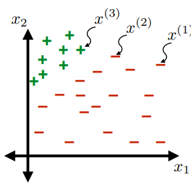
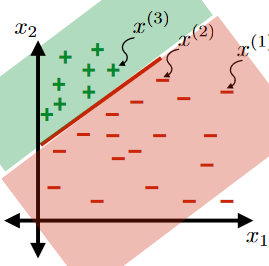
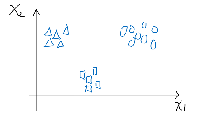
Consider an example of predicting whether if a newborn baby in the hospital will have a seizure.

We are provided beforehand with:

$n$ training data points
\[\mathcal{D}_n = \{ (x^{(1)}, y^{(1)}), ..., (x^{(n)}, y^{(n)}) \}\]
- each data point, $x^{(i)}, i \in {1,…,n}$ is a feature vector, so that $x^{(i)} \in \mathbb{R}^d$
  - for example, $x^{(i)}_1$ could represent the amount of oxygen the baby is breathing, and $x^{(i)}_2$ could represent the amount of movement the baby has
- each data point, $x^{(i)}$ has a corresponding label, $y^{(i)} \in {-1,+1}$, so that
  - $-1$ means newborn baby $i$ did not have a seizure
  - and $+1$ means newborn baby $i$ did have a seizure

So that we have the following:

in this simple example, $d=2$

Questions to Answer

How can we label those points?
What are good ways to label them?

Possible Solutions

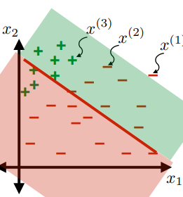
Labeling Hypothesis: we need a “function” $h$ that does:
\[h: \mathbb{R}^d \mapsto \{-1, +1\}\]
Linear Classifiers is a good set of hypothesis to use.
- e.g. the hypothesis class $\mathcal{H}: \text{set of }h \in \mathcal{H}$ such that:
  - labels $+1$ on one side of a line, and $-1$ on the other side of the line

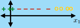
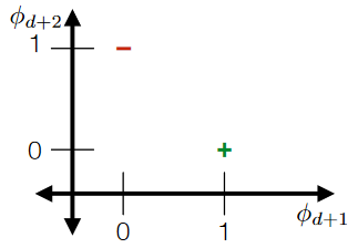
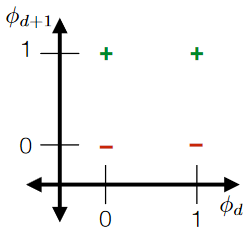
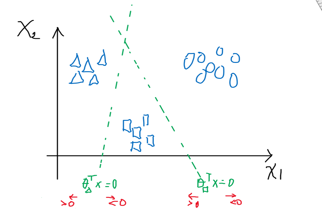
Linear Classifiers

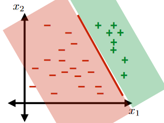
For the same given (training) data:

Consider the hypothesis class $\mathcal{H}= \text{set of }h \in \mathcal{H}$ such that:

labels $+1$ on one side of a line, and $-1$ on the other side of the line
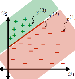
below are some hypothesis in this class $\mathcal{H}$

| | | | ———————————————————— | ———————————————————— |

Review

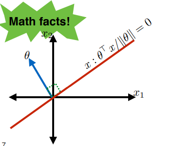
Recall that if we have the two vectors $\theta, x$:

then the dot product:
\[\frac{x \cdot \theta}{||\theta||} = \frac{x^T \theta }{||\theta||}\]
represents the projection of $x$ onto $\theta$.

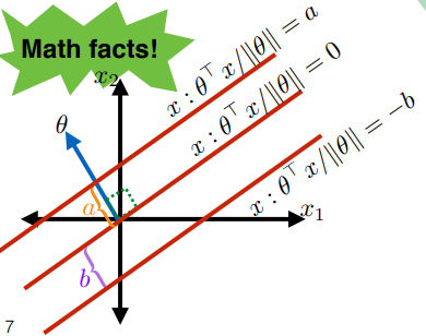
Therefore, an important point is that:

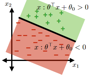
where the red line (set of $x$) can be represented by:
\[x : \frac{\theta \cdot x}{||\theta||} = 0\]
and that:
\[\begin{align*} x : \frac{\theta \cdot x}{||\theta||} &= a \\ x : \frac{\theta \cdot x}{||\theta||} &= -b \end{align*}\]
defines the following additional two lines:

where the advantage of defining lines here is that:

all we used are data points

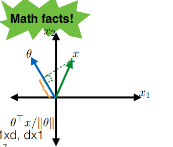
Therefore, we can say that for we can describe any line in 2 dimension as:

\[\begin{align*} \frac{\theta^T x}{||\theta||} &= -b \\ \theta^T x + b ||\theta|| &= 0\\ \theta^T x + \theta_0 &= 0 \end{align*}\]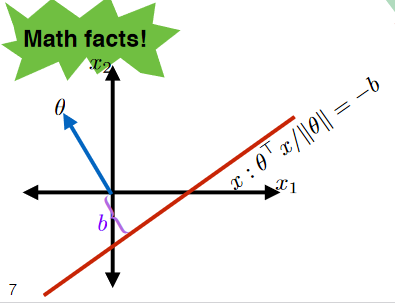

So the linear classifier can just look at the sign of $x$ relative to the line

\[h(x) = h(x; \theta, \theta_0)=\text{sign}(\theta^T x + \theta_0) = \begin{cases} +1, & \text{if } \theta^T x + \theta_0 > 0\\ -1, & \text{if } \theta^T x + \theta_0 \le 0\\ \end{cases}\]

where:

the equality $\le$ is arbitrary. It could be applied on $>$ alternatively.
$h(x; \theta, \theta_0)$ means $h$ is a function of input $x$, with parameter $\theta, \theta_0$ that has nothing to do with input

Now, we can define the linear classifier class to be:

\[\mathcal{H} = \{h(x;\theta, \theta_0), \forall \theta, \theta_0\}\]

where again the input is $x$

Note:

At this point, all that we have to do is:

be able to evaluate how good a hypothesis $h$ is
be able to find the best $h$ in the class

Evaluating a Classifier

Note:

This discussion applies to the general case of any classifier

To be able to determine if a hypothesis is good or not, we can look at the loss function:

\[L(g,a)\]

where:

$g$ means the our guess from hypothesis
$a$ means the actual value
note that it does not depend on input, since this basically just describes how bad it is if we guessed incorrectly

For Example:

Symmetric Loss

\[L(g,a) = \begin{cases} 0, & \text{if }g =a \text{, i.e. guessed correctly}\\ 1, &\text{otherwise} \end{cases}\]

however, a better loss might be:

\[L(g,a) = \begin{cases} 0, & \text{if }g =a \text{, i.e. guessed correctly}\\ 1, & \text{if }g=1,a=-1\\ 100, &\text{if }g=-1,a=1 \end{cases}\]

where:

$g=-1,a=1$ represents we predicting newborn NOT having a seizure, but they actually had. Therefore, it is detrimental and weighted more.

Therefore, we can define:

Test Error

For $n’$ points of new data, the test error of a hypothesis $h$ is:
\[\mathcal{E}(h) = \frac{1}{n'} \sum_{i=n+1}^{n+n'}L(h(x^{(i)}), y^{(i)})\]
where basically:

we are averaging over the loss function, and the guess comes from the hypothesis $h$

Training Error

For $n$ points of old/given data, the training error of a hypothesis $h$ is:
\[\mathcal{E}_n(h) = \frac{1}{n} \sum_{i=1}^{n}L(h(x^{(i)}), y^{(i)})\]
where basically:

we are using existing data as input for $h$

Then, we can say I prefer hypothesis $h$ over $\bar{h}$ if (for example):

\[\mathcal{E}_n(h) < \mathcal{E}_n(\bar{h})\]

i.e. $h$ has a smaller training error (common) than $\bar{h}$

Picking a Classifier

Obviously we cannot just try out every classifier and compute the $\mathcal{E}$. Therefore, we think about

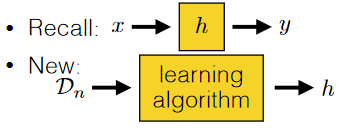
So in general, this is what is happening:

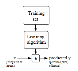
where:

the output of your algorithm is a hypothesis, which is basically a function that can give you predicted output based on some input

where we can use a learning algorithm to spit out a *good* classifier by:

taking in an entire dataset $\mathcal{D_n}$

e.g.

| | | | :———————————————————-: | :———————————————————-: |

For Example

Your hypothesis class is generated by your friend to be:

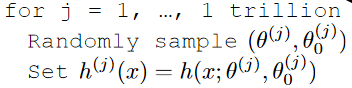
where basically you get a trillion hypothesis.

A simple learning algorithm would be:

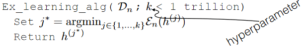
where:

$k$ is a hyperparameter, which does not change the logic of algorithm at all. It is just a parameter we can choose as programmer
we basically found $h^{(j^*)}$ such that it has the smallest training error among $k$ classifiers

Note:

notice that it means $\text{Ex_learning_alg}(\mathcal{D}_n;2)$ must output an algorithm that is at least as good as $\text{Ex_learning_alg}(\mathcal{D}_n;1)$.
this means that as $k$ increases, we will get better classifiers

In practice, if we took:

\[L(g,a) = \begin{cases} 0, & \text{if }g =a \text{, i.e. guessed correctly}\\ 1, &\text{otherwise} \end{cases}\]

and that we use training error to decide upon the better hypothesis.

Then the process of $\text{Ex_learning_alg}(\mathcal{D}_n;k)$ looks like:

On the first run with $h^{1}$

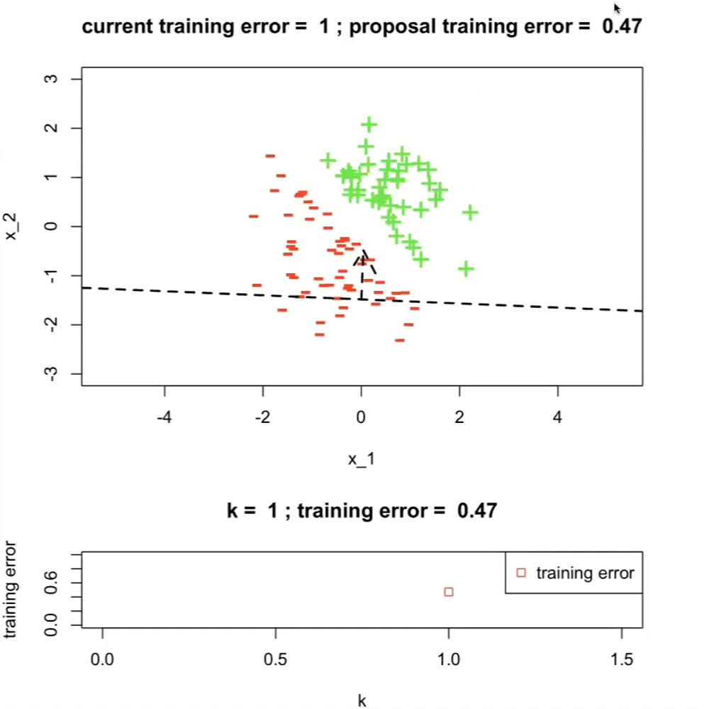
where the top graph has:
- a dotted line indicating our hypothesis $h^{(1)}$
- current training error set to $1$ which is the maximum
- $h^{(1)}$ is having a training error of $0.47$
the bottom graph is the plot of training errors with respect to $k$-th hypothesis
- therefore $j^*=1$ currently
The next proposal/hypothesis $h^{(2)}$ has a better training error:

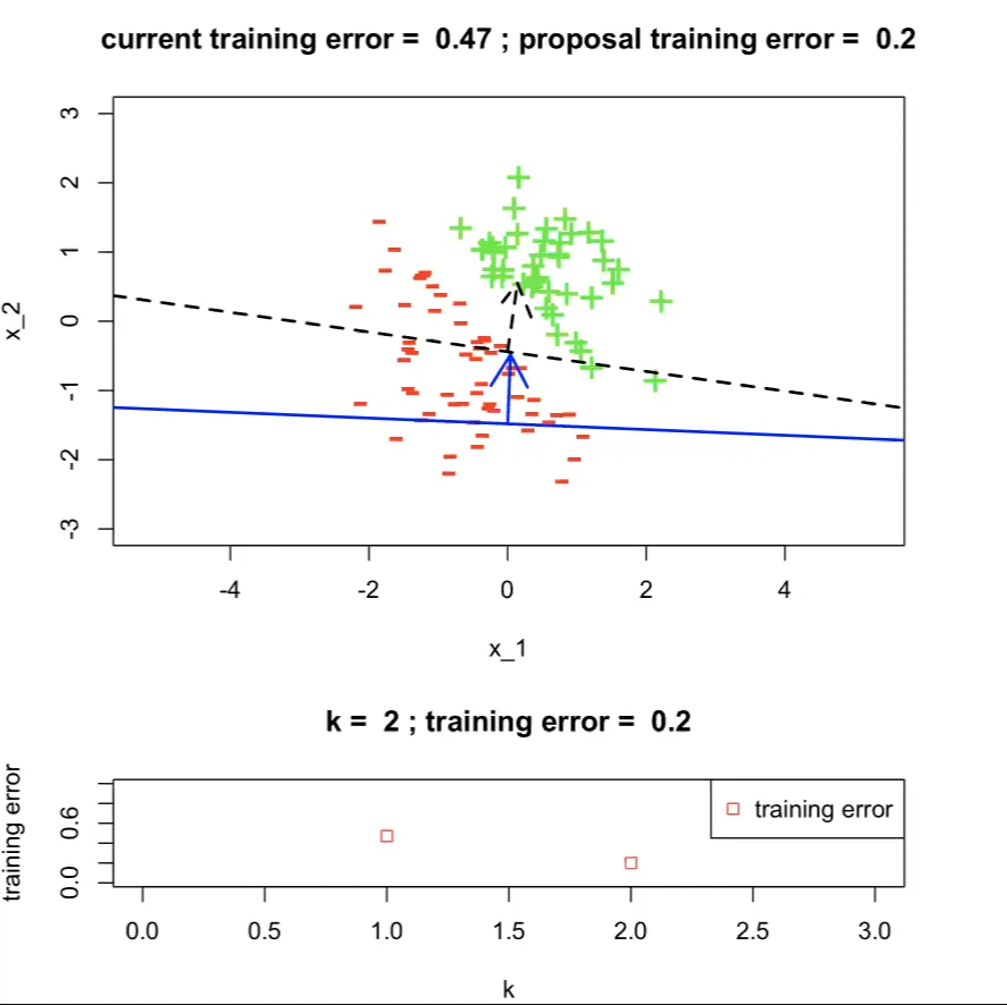
now $j^*=2$
….
Over 413 runs, we get up to $0.01$ for error. But obviously there is one that would give $\mathcal{E}(h)=0$

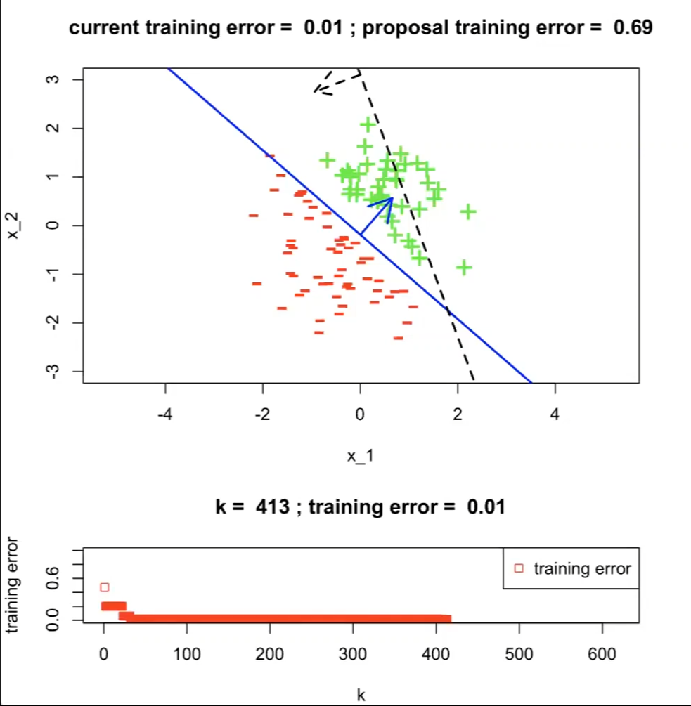
Therefore, we kind of need a better learning algorithm

Machine Learning Techniques

The examples in the last lecture talks about problem of classification, to be specific, a binary classification.

classDiagram
	Supervised_Learning <|-- Regression
	Supervised_Learning <|-- Classification
	Unsupervised_Learning <|-- _
	Classification <|-- Binary_Classification
	Classification <|-- Multi_Class_Classification

Classification:

Learning an input mapping to a discrete set
\[\mathbb{R}^d \mapsto \{...\}\]
where:

input is $\mathbb{R}^d$

output is ${…}$

In specific, what we have met is the binary classification:

Binary Classification

Learning an input mapping to a discrete set of two values
\[\mathbb{R}^d \mapsto \{-1,+1\}\]

for example, we can have a linear classifier (i.e. a hyperplane) to solve such problem

Multi-class Classification

Learning an input mapping to a discrete set of more than two values

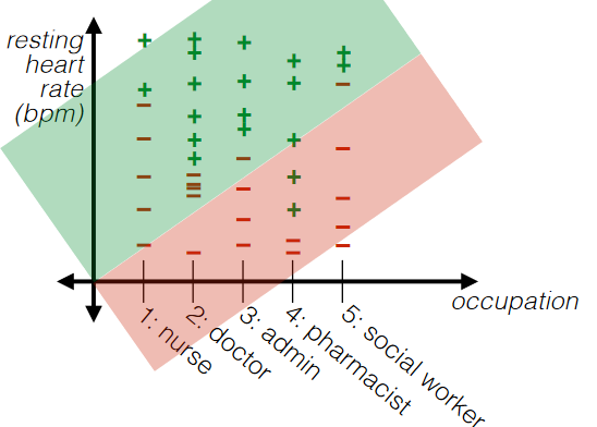
e.g.

usually in this case, a linear classifier would not work properly

In other cases, we might want get some continuous output. For example, the real-time temperature in a room. Then we usually use regression

Regression

Learning an input mapping to continuous values
\[\mathbb{R}^d \mapsto \mathbb{R}^k\]
e.g.

Lastly, unsupervised learning talks about:

Unsupervised Learning

No labels for input. The aim is to find patterns in a given dataset.

General Steps for ML Analysis

In general, you would have needed to:

Establish a goal & find data
- Example goal: diagnose whether people have heart disease based on their available information
Encode data in useful form for the ML algorithm
- some sort of transformation (i.e. feature function) to the dataset
Run the ML algorithm & return a classifier (i.e. a function/hypothesis $h$)
- if the problem is supervised learning
- Example algorithms include perceptron algorithm, average perceptron algorithm, etc.
Interpretation and Evaluation

Feature:

A function that takes the input/raw data and converts it to some ML usable form for later processing
\[x \mapsto \phi(x)\]

for example, one hot encoding (see section below)

Note:

sometimes, feature functions $\phi(x)$ are just referred to as features $\phi$, since it is usually the resulting value/vector that we care about in ML
Those feature functions does not have to be reversible

Example

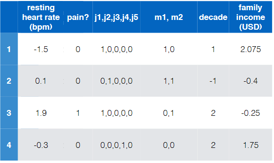
Consider the task of diagnose whether people have heart disease based on their available information

First, need goal & data

e.g.

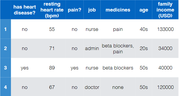
where notice that:

there are of course more data to these four
this is labelled and is binary (has heart disease?)
- so this is a binary/two-class classification
the input features are basically all the rest

Note that:

Even if we have the input features ready, we need to find some way to convert string (non-numeric) information to numbers. Otherwise we cannot use our established models

Encode data in a usable form

We can easily convert the labels=”has heart disease” to:
\[\{\text{'yes'}, \text{'no'}\} \iff \{ +1,-1 \}\]

The data/inputs needs some work. We need to use some feature $\phi$ that:

\[x \mapsto \phi(x)\]

where:

old/raw features is $x$
new feature for ML is $\phi(x)$

e.g.

some interesting encoding to see would be:

where:
- this is also called a one hot encoding
and factored encoding (since there are overlaps):

Overall:

$x$, old data/feature	$\phi(x)$, new data/feature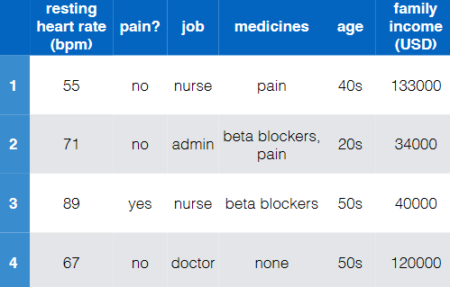

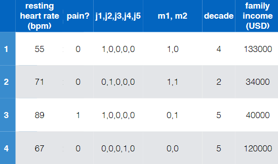
Note

In step 2, some other ideas could be:

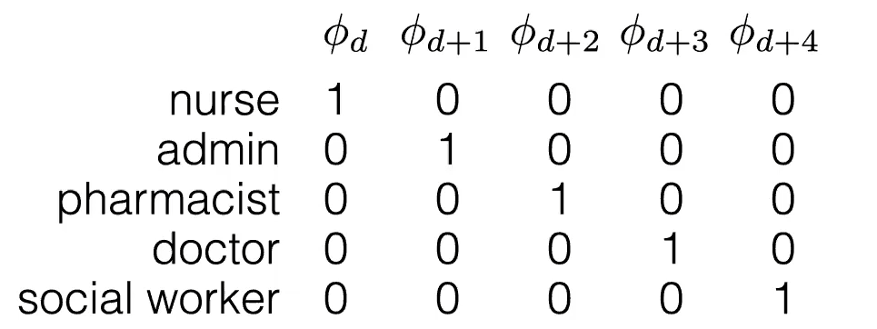
For categorial jobs:
1. if we turned categorial information into some unique natural numbers:
  
  then we are imposing some sort of ORDERINGS to the categories. This sometimes is not a good idea.
2. A good idea is to turn each category into a unique feature. For example:
  
  then the advantage is that you can always "separate/group" those categories as they are always “apart”
For overlapping “categories”:
1. Notice that since there are overlaps, something like this would be nice:
  
  such that it should still be separable (think about cases when it is not):
Note
- this is strictly different from a binary encoding, because we kind of chose some useful orderings/groupings to show those overlaps.

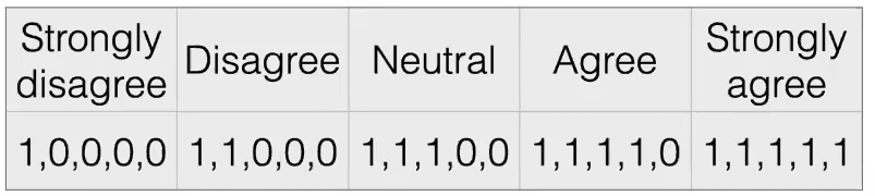
Encode Ordinal Data

In general, you would meet three kinds of data to go through your feature (function):

Numerical Data: order on data values, and differences in value are meaningful
- e.g. heart rate = 56, 67, 60, etc
- e.g. filtering useless ones; standardization
Categorical Data: no order information
- e.g. job = doctor, nurse, pharmacist
- e.g. one hot encoding
Ordinal Data: order on data values, but differences not meaningful without some processing
- e.g. Likert Scale
  
  is the difference between each state exactly the same?

For Example

Unary/Thermometer Code

$x$	$\phi(x)$

where notice that the advantage is:

order information still exists
difference information is “removed”

For Example: Filtering

Even numerical data could be useless. Consider

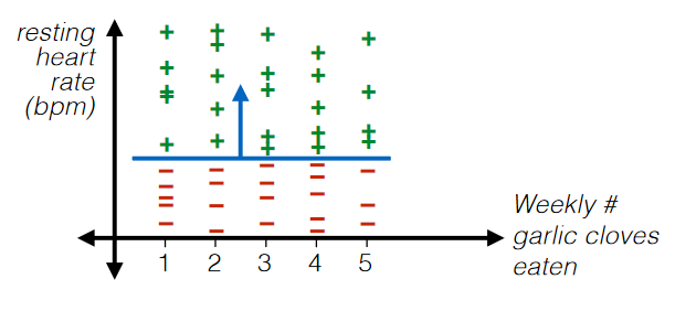
where:

in this case, “Weekly # Garlic Clove Eaten” is useless
maybe ask some experts on this. This might be important unless you are sure.

For Example: Standardization

$x$	$\phi(x)$

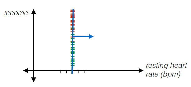where basically each data point has gone through:

Standardization

Given some data point $x^{(d)} \in \mathcal{D}_n$:
\[\phi_d^{(k)} = \frac{x_d^{(k)}-\text{mean}_d}{\text{stddev}_d}\]
where:

doing $\frac{1}{\text{stddev}_d}$ basically zooms in the data

where the advantage of this is that:

such classifier would be independent of the scale of axis that you chose to plot at
also, it would sometimes be easier to interpret the result/classifier

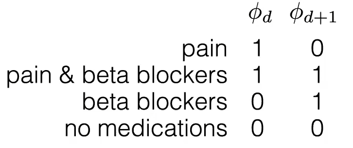
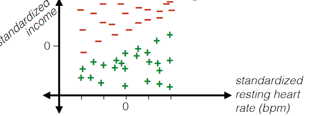
Therefore, we could further encode the example in the previous lecture to be:

$x$	$\phi(x)$

where notice that:

“resting heart rate” and “family income (USD)” has now been standardized

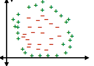
Nonlinear Boundaries

Review

Recall that a plane can be defined a point $\vec{r}_0$ in the plane AND its normal vector $\vec{n}$:
\[\begin{align*} \vec{n} \cdot (\vec{r}-\vec{r}_0) &= 0 \\ \vec{n} \cdot \vec{r} &= \vec{n} \cdot \vec{r}_0 \end{align*}\]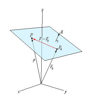

where:
- $\vec{r}$ basically is “input”
- $\vec{n}\cdot \vec{r}_0$ basically is a constant

Therefore, consider classifying:

where now your “hyperplane classifier” is:

$\theta^T x + \theta_0 = 0$, $x \in \mathbb{R}^2$

By adding a new dimension $z$, and then you have

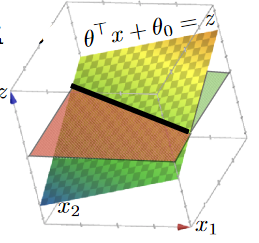
now your “hyperplane classifier” becomes:

$\theta^T x + \theta_0 = z$, $x \in \mathbb{R}^2$

An advantage of this idea is to classify:

dataset	hyperplane/classifier: $f(x)=z,x\in \mathbb{R}^2$

Linear Regression

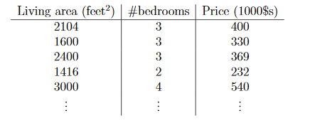
Consider the following data:

where:

$x^{(i)}_1$is the living area of the $i$-th house in the training set, and $x^{(i)}_2$ is its number of bedrooms.
$y$ is a continuous (assuming continuous price) output
since output/labels are given, this is supervised learning

Then, an example would be to use linear regression

\[h(x;\theta)=h_\theta(x) = \theta_0 + \theta_1 x_1 + \theta_2 x_2\]

Alternatively, letting $x_0\equiv 1$, we can have a compacter form:

\[h(x) = \sum_{i=0}^n \theta_i x_i = \theta^T x\]

where now we basically have:

input/feature $x=\begin{bmatrix} 1 \x_1 \x_2 \ \end{bmatrix}=\begin{bmatrix} x_0 \x_1 \x_2 \ \end{bmatrix}$
parameter $\theta = \begin{bmatrix} \theta_0 \\theta_1 \\theta_2 \ \end{bmatrix}$ would be the job of Learning Algorithm to choose

Therefore, the task of Learning Algorithm is to decide $\theta$ such that $h(x) \approx y$ for $x \in \mathcal{D}_m$ being the training dataset consisting of $m$ data pairs.

Some sensible idea would be to minimize the square of the error:

Gradient Descent Algorithm
Normal Equation

LMS Algorithm

The aim of Learning Algorithm is to decide $\theta$ such that $h(x) \approx y$ for $x \in \mathcal{D}_m$ being the training dataset consisting of $m$ data pairs.

LMS Algorithm

We first define the cost function $J$ to be:
\[J(\theta) = \frac{1}{2} \sum_{i=1}^{m}\left( h_\theta(x^{(i)})-y^{(i)} \right)^2\]
where:

the $\frac{1}{2}$ there is just so that taking derivatives later would look nicer

Therefore, now the aim is to choose $\theta$ to minimize $J(\theta)$

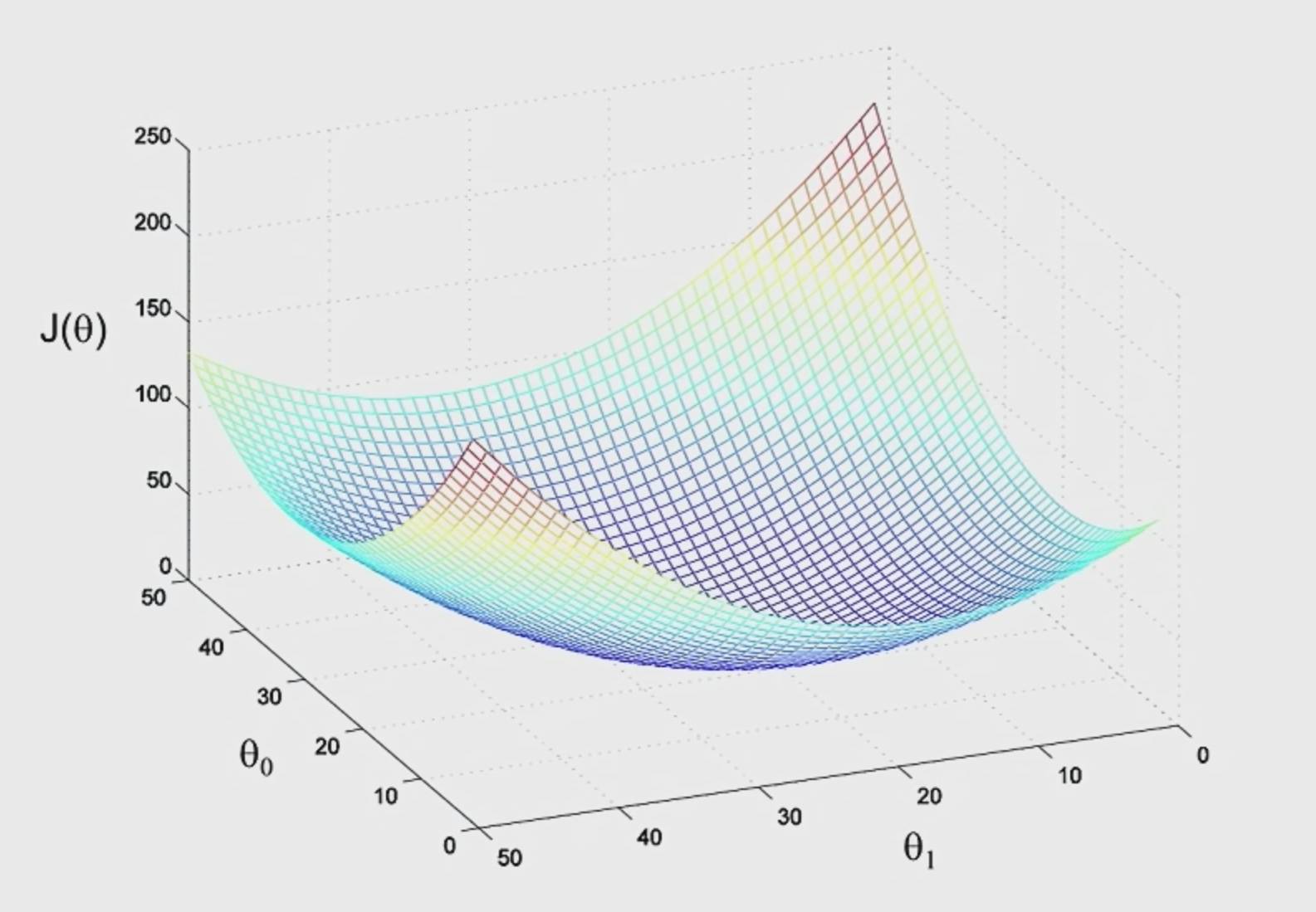
Batch Gradient Descent Algorithm

To achieve this, one way is to use (Batch) Gradient Descent Algorithm.

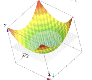
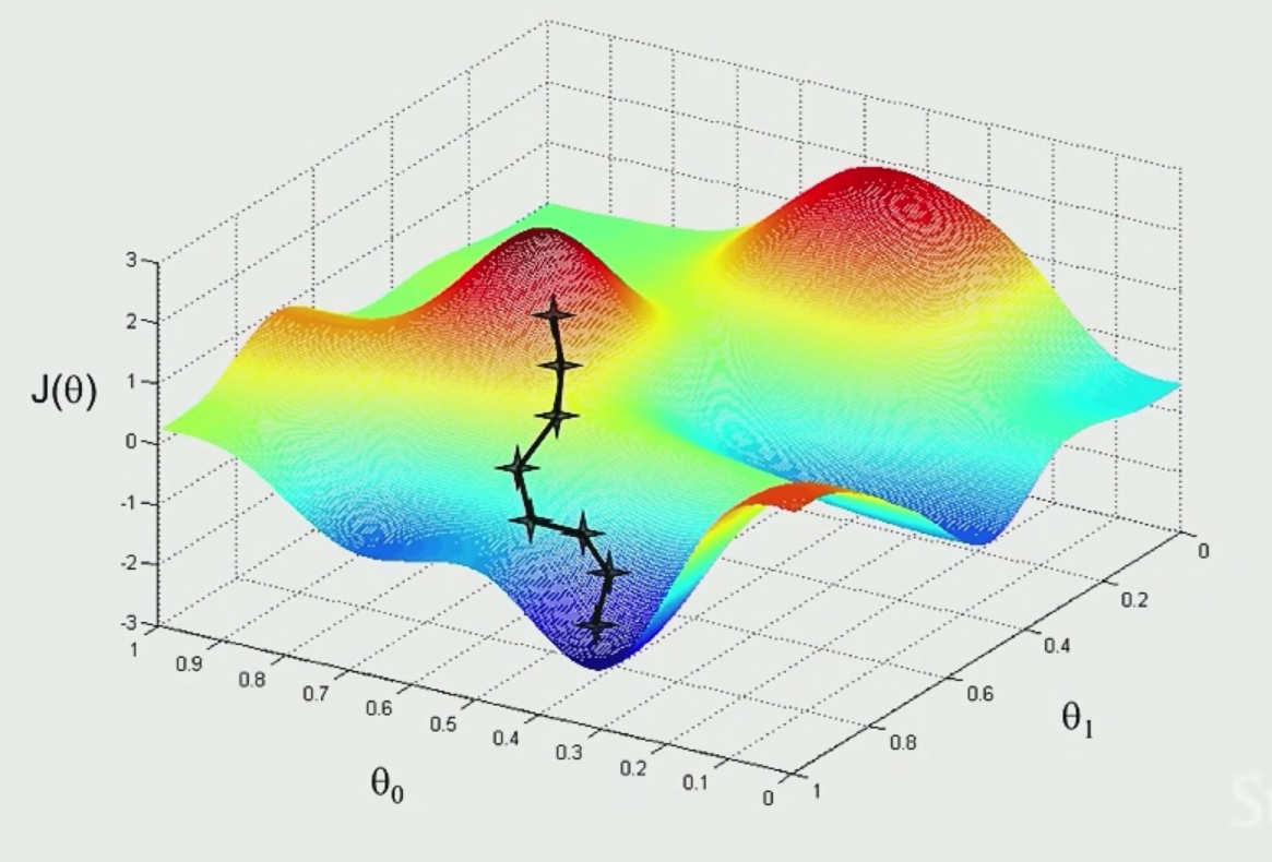
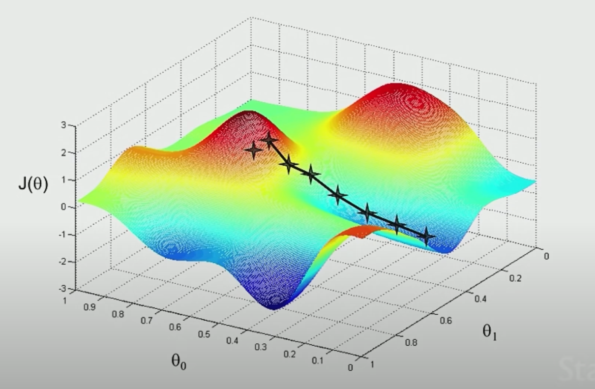
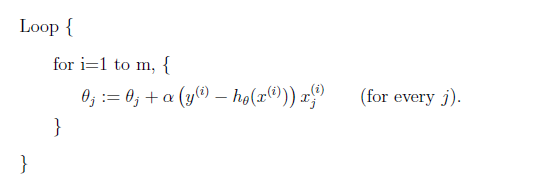
The idea is that if we plot $\theta_1,\theta_2$ and $J$ (not the $J$ defined above, which should be a convex function), we see something like:

| | | | :———————————————————-: | :———————————————————-: |

where the aim is to find the minima point:

pick some point to start with
for each point, decide where to move down next based on gradient vector
move in that direction and repeat step 2

However, notice that the final local minima sometimes depends on where you start with.

Gradient Descent Algorithm

Basically start with some initial $\theta=\begin{bmatrix}\theta_0 \ \theta_1 \ …\end{bmatrix}$, and then repeatedly move, $\forall j$:
\[\begin{align*} \theta_j &:=\theta_j - \alpha \frac{\partial}{\partial \theta_j} J(\theta) \\ &=\theta_j - \alpha \sum_{i=1}^m \left[ \left(h_\theta(x^{(i)})-y^{(i)}\right)x_j^{(i)} \right]\\ \end{align*}\]
where:

$:=$ is the assignment, which takes value from the right and assign it to the left

$\alpha$ is called the learning rate, usually set to $0.01$ and manipulate around

the $-\alpha$ indicates that we are moving DOWN the slope to minima.

This method looks at every data point in the entire training set for each step (of computing the next $\theta_j$ value), and is called batch gradient descent (i.e. so a batch here would mean the entire dataset $\mathcal{D}_m$).

Then you repeat until convergence

notice that the definition of $J$ would cause our function to only have one global minimum. Therefore with appropriate $\alpha$, you should always get your data to converge
\[J(\theta) = \frac{1}{2} \sum_{i=1}^{m}\left( h_\theta(x^{(i)})-y^{(i)} \right)^2\]

note that this is a convex function. This is because the sum of convex function $\left( h_\theta(x^{(i)})-y^{(i)} \right)^2$ is still a convex function. (for a simple case, consider the sum of quadratics still being a quadratic)

Therefore $J$ typically looks like:

So in summary, this algorithm does:

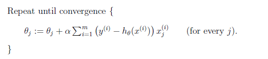
Note:

If we plot the contour, then the gradient will always look like:

where:
- basically we are moving perpendicular (gradient) to the contours
This also implies some choice of $\alpha$
- if you choose your $\alpha$ to be too large, then the last steps might overshoot pass the minima
- if you choose your $\alpha$ to be too small, then you need a lot of iterations to get to the minima

Proof

Consider the case when there is only one data point in $\mathcal{D}_m$, then:

\[\begin{align*} \theta_j &:=\theta_j - \alpha \frac{\partial}{\partial \theta_j} J(\theta) \\ &:=\theta_j - \alpha \frac{\partial}{\partial \theta_j} \left( \frac{1}{2} (h_\theta(x) - y)^2\right)\\ &:=\theta_j - \alpha (h_\theta (x) - y)\frac{\partial}{\partial\theta_j}(h_\theta(x)-y)\\ &:=\theta_j - \alpha (h_\theta (x) - y)\frac{\partial}{\partial\theta_j}(\theta^Tx-y)\\ &:=\theta_j - \alpha (h_\theta (x) - y)\frac{\partial}{\partial\theta_j}\left[ (\theta_0 x_0 + \theta_1x_1+...) -y\right]\\ &:=\theta_j - \alpha (h_\theta (x) - y)x_j \end{align*}\]

Now, if you take all the data points, recall that:

\[\begin{align*} \frac{\partial}{\partial \theta_j} \left( \sum_{i=1}^m \frac{1}{2} (h_\theta(x^{(i)}) - y^{(i)})^2\right) &=\sum_{i=1}^m\frac{\partial}{\partial \theta_j} \left( \frac{1}{2} (h_\theta(x^{(i)}) - y^{(i)})^2\right)\\ &=\sum_{i=1}^m \left[ \left(h_\theta(x^{(i)})-y^{(i)}\right)x_j^{(i)} \right]\\ \end{align*}\]

Therefore you get:

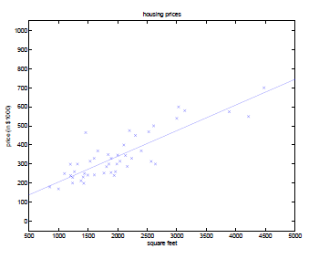
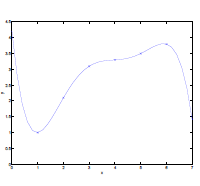
\[\begin{align*} \theta_j &:=\theta_j - \alpha \frac{\partial}{\partial \theta_j} J(\theta) \\ &=\theta_j - \alpha \sum_{i=1}^m \left[ \left(h_\theta(x^{(i)})-y^{(i)}\right)x_j^{(i)} \right]\\ \end{align*}\]

In the example of:

The gradient descent algorithm will result in a $\theta$ such that our line looks like:

Problem of Gradient Descent

This method of Gradient Descent looks at every data point in the entire training set for each step (i.e. so a batch here would mean the entire dataset $\mathcal{D}_m$). This means we for each step, we need to compute for all data points, which is very expensive if there are a lot of data points.

Stochastic Gradient Descent Algorithm

Stochastic Gradient Descent Algorithm

Instead of making one update for every scan through dataset, we can make one update per data point. Therefore, the algorithm looks like:

where:

in practice, this does make you move faster towards the minima

However, the upshot of this is that it may never converge, since you are now only updating per each data point

this could be “minimized” by continuously decreasing the learning rate $\alpha$, so that the oscillation would be slower

The Normal Equation

Gradient descent gives one way of minimizing $J$. A second way of doing so is to perform the minimization explicitly and without resorting to an iterative algorithm.

therefore, this is much faster than the algorithms above
but this works iff there is a solution

Recall/Notations

if you have $J(\theta)$, where input $\theta \in \mathbb{R}^{m+1}$, then, if for example $m=2$, we have:
\[\nabla_\theta J(\theta) = \begin{bmatrix} \frac{\partial }{\partial \theta_1}J\\ \frac{\partial }{\partial \theta_2}J\\ \frac{\partial }{\partial \theta_3}J \end{bmatrix}\]
now, you can also have input as matrix, e.g. input being $A \in \mathbb{R}^{2 \times 2}$ sand that a function $f$ maps $f:\mathbb{R}^{2\times 2} \to \mathbb{R}$
\[\nabla_A f(A) = \begin{bmatrix} \frac{\partial f}{\partial A_{11}} & \frac{\partial f}{\partial A_{12}}\\ \frac{\partial f}{\partial A_{21}} & \frac{\partial f}{\partial A_{22}} \end{bmatrix}\]
If we have a square matrix $A \in \mathbb{R}^{n \times n}$, then the trace of $A$ $\text{tr}(A)$ is:
\[\text{tr}(A) = \sum_{i=1}^n A_{ii}\]
some common properties:
1. $\text{tr}ABC=\text{tr}CAB=\text{tr}BCA$
2. $\nabla_A \text{tr}AB = B^T$
3. $\nabla_{A^T}f(A) = (\nabla_A f(A))^T$
4. $\nabla_A \text{tr} AA^TC = CA+C^TA$
5. $\nabla_A \text{tr}ABA^TC = CAB + C^TAB^T$
  - from 2 and 3 above
6. $\nabla_A\vert A\vert = \vert A\vert (A^{-1})^T$

The aim is to achieve:

\[\nabla_\theta J(\theta) = 0\]

but:

computing it directly might be expensive since $J(\theta)$ needs to look through all data

Then consider the design matrix, which is $X$ by stacking input data point $x^{(i)} \in \mathbb{R}^{n+1}$ to be:

\[X = \begin{bmatrix} -(x^{(1)})^T- \\ -(x^{(2)})^T-\\ \vdots \\ -(x^{(m)})^T- \end{bmatrix}\]

where:

$X \in \mathbb{R}^{m \times (n+1)}$

Similarly, define the labels to be:

\[\vec{y} = \begin{bmatrix} y^{(1)} \\ y^{(2)}\\ \vdots \\ y^{(m)} \end{bmatrix}\]

Therefore, we have:

\[\begin{align*} X\theta &=\begin{bmatrix} -(x^{(1)})^T- \\ -(x^{(2)})^T-\\ \vdots \\ -(x^{(m)})^T- \end{bmatrix}\begin{bmatrix} \theta_1 \\ \theta_2\\ \vdots \\ \theta_n \end{bmatrix} = \begin{bmatrix} (x^{(1)})^T \theta \\ (x^{(2)})^T \theta \\ \vdots\\ (x^{(m)})^T \theta \end{bmatrix} = \begin{bmatrix} h_\theta(x^{(1)})\\ h_\theta(x^{(2)}) \\ \vdots\\ h_\theta(x^{(m)}) \end{bmatrix}\\ \end{align*}\]

And more importantly:

\[\begin{align*} J(\theta) &= \frac{1}{2} \sum_{i=1}^m (h_\theta(x^{(i)})-y^{(i)})^2 \\ &= \frac{1}{2} (X\theta -\vec{y})^T(X\theta -\vec{y}) \end{align*}\]

Normal Equation

Therefore, since we are finding the minimum point, we basically just do:
\[\begin{align*} \nabla_\theta J(\theta) &= 0\\ X^T (X\theta - \vec{y}) &= 0 \end{align*}\]
where:

$X^T (X\theta - \vec{y}) = 0$ is the also called the normal equation

The solution $\theta$ therefore satisfies:
\[\theta = (X^TX)^{-1}X^T \vec{y}\]

Proof

we already know that:

\[\begin{align*} J(\theta) &= \frac{1}{2} \sum_{i=1}^m (h_\theta(x^{(i)})-y^{(i)})^2 \\ &= \frac{1}{2} (X\theta -\vec{y})^T(X\theta -\vec{y}) \end{align*}\]

Then:

\[\begin{align*} \nabla_\theta J(\theta) &= \nabla_\theta\frac{1}{2} (X\theta -\vec{y})^T(X\theta -\vec{y}) \\ &= \frac{1}{2}\nabla_\theta (\theta^TX^T -\vec{y}^T)(X\theta -\vec{y}) \\ &= \frac{1}{2}\nabla_\theta (\theta^TX^T X\theta -\vec{y}^T X\theta -\theta^TX^T \vec{y} + \vec{y}^T\vec{y}) \\ &= \frac{1}{2}\nabla_\theta \text{tr}(\theta^TX^T X\theta -\vec{y}^T X\theta -\theta^TX^T \vec{y} + \vec{y}^T\vec{y}) \\ &= \frac{1}{2}\nabla_\theta (\text{tr }\theta^TX^T X\theta -2\text{tr }\vec{y}^TX\theta) \\ &= \frac{1}{2}\left( X^TX\theta + X^TX\theta -2X^T \vec{y} \right)\\ &= X^TX \theta - X^T \vec{y} \end{align*}\]

Therefore, setting it to zero gives:

\[\begin{align*} \nabla_\theta J(\theta) = X^TX \theta - X^T \vec{y} &= 0\\ X^T (X\theta - \vec{y}) &= 0 \end{align*}\]

Therefore, the optimum value for $\theta$ becomes:

\[\begin{align*} X^T X\theta &= X^T \vec{y}\\ \theta &= (X^TX)^{-1}X^T \vec{y} \end{align*}\]

Nonlinear Fits

Now suppose you want to fit some of your data in a nonlinear form.

Or even:

\[\theta_0 + \theta_1 x^{(i)}_1 + \theta_2 \sqrt{x^{(i)}_2} + \theta_3 \log x^{(i)}_3\]

What you can do is simply:

let $x^{(i)}_2 := \sqrt{x^{(i)}_2}$, let $x^{(i)}_3 := \log x^{(i)}_3$
then you are backed to a linear regression problem, and can apply the same techniques as above

Problem

the problem with this is that you need to know which equation in advance. e.g. are you sure it is square root for a feature $x^{(i)}_2$? Logarithmic for $x^{(i)}_3$? etc.

Overfitting and Underfitting

The idea for both is common but straight-forward

Underfitting: model has not captured the structure for data in the training set
Overfitting: model imitated the data but NOT the structure. i.e. the data is distributed in $x^2$, but $x^3$, or $x^4$ is used.

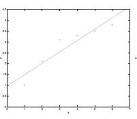
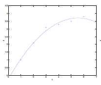
For Example:

Consider the data being actually distributed in $x \mapsto O(x^2)$, such that we have:

Underfitting	Actual	Overfitting

where:

first figure is underfitted as we only imagined $y = \theta_0 + \theta_1 x$.
third figure is overfitting as we imaged $y=\theta_0 + \theta_1 x + \theta_2 x^2 + … + \theta_5 x^5$
- we could interpret this as having five features, $x_1 = x,\,x_2 = x^2,\,x_3=x^3,\,…\,x_5=x^5$,and fitting them all in a linear manner
These notions will be formalized later.

Take-away Message

the choice of features/hypothesis is important to ensuring good performance of a learning algorithm. (When we talk about model selection, we’ll also see algorithms for automatically choosing a good set of features.)

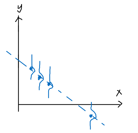
Locally Weighted Linear Regression

Advantage for Overfitting

One advantage of locally weighted linear regression (LWR) algorithm is, assuming there is sufficient training data, makes the choice of features less critical. (as it is a local model)

The Linear Regression discussed in section Linear Regression is a type of “Parametric” Learning Algorithm, because the output/aim is a fixed size of parameters $\theta = \begin{bmatrix} \theta_0 \\\vdots\\\theta_n \\ \end{bmatrix}$ to a dataset

this means that the output ($\theta$) is constant in size for any dataset

However, the LWR (Locally Weighted Linear Regression) would be “Non-parametric” Learning Algorithm, because the output/aim are parameters that grows/increases linearly with size of dataset

this means that you can easily fit nonlinear dataset, but the output might be large for large dataset

The idea of LWR is as follows.

Consider the following dataset:

where, for each desired output of an input $x$, we consider:

mostly importantly the neighborhood around/near the input $x$
slightly consider (less weight) on the data far away from the input $x$
Fit $\theta$ that minimizes $J$ using the above two steps

LWR

Instead, we have the error function $J$ to be:
\[J(\theta) = \frac{1}{2} \sum_{i=1}^{m} w^{(i)}\left( h_\theta(x^{(i)})-y^{(i)} \right)^2\]
where:

basically we are adding weight $w^{(i)}$ to each data point,

A common $w$ to use is:
\[w^{(i)} = \exp{\left(-\frac{(x^{(i)}-x)^2}{2\tau^2}\right)}\]
so that:

$x$ is the input which we want to get the prediction of

so if $x$ is close to some points $x^{(i)}$, then the weight is close to $1$. Otherwise, far away points have weight close to $0$

$\tau$ specifies the width of the bell shaped curve, and is called the bandwidth parameter. This will be a hyper-parameter.

Therefore, performing $J(\theta)$ means:

we are “only” computing prediction errors near input point $x$

Probabilistic Interpretation

This section aims to answer questions such as:

Why using Least Squares for Error?

Consider the case for housing data:

And assuming the actual distribution of data is:

\[y^{(i)} = \theta^T x^{(i)} + \epsilon^{(i)}\]

where:

so housing prices is a linear function on the features
$\epsilon^{(i)}$ means the error term that captures either unmodeled effects or random noise.
- e.g. the seller’s mood on that day

Pictorially

Model:	Actual Data:

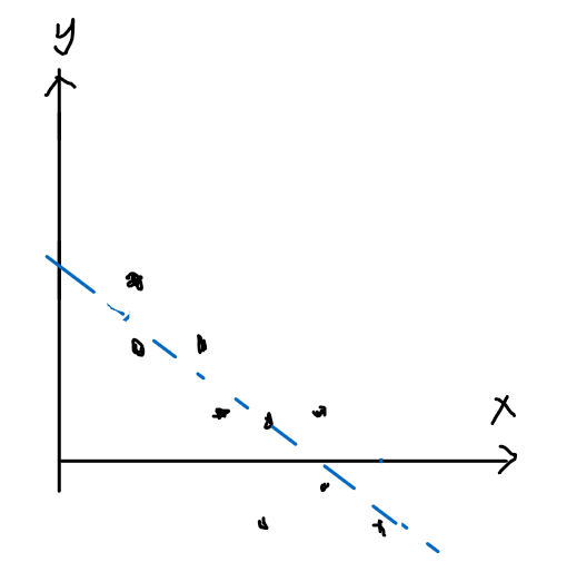And that we assume the error term $\epsilon^{(i)}$ is distributed IID (independently and identically distributed according to a Gaussian Distribution, also called a Normal Distribution):

\[\epsilon^{(i)} \sim \mathcal{N}(0, \sigma^2)\]

where this normal distribution has:

mean being $0$
standard deviation of $\sigma$
in general, for those types of data, the distributions would be Gaussian due to the Central Limit Theorem

So that this means the density of $\epsilon^{(i)}$ is given by:

\[p(\epsilon^{(i)}) = \frac{1}{\sqrt{2\pi} \sigma} \exp{\left( - \frac{(\epsilon^{(i)})^2}{2 \sigma^2} \right)}\]

Therefore, since now we know the density of $\epsilon^{(i)}$ and we know $y^{(i)} = \theta^T x^{(i)} + \epsilon^{(i)}$, this gives:

\[p(y^{(i)} | x^{(i)}; \theta) = \frac{1}{\sqrt{2\pi} \sigma} \exp{\left( - \frac{(y^{(i)} - \theta^T x^{(i)})^2}{2 \sigma^2} \right)}\]

where:

$p(y^{(i)} \vert x^{(i)}; \theta)$ means the distribution of $y^{(i)}$ given $x^{(i)}$ and parametrized by $\theta$
- so only $x^{(i)}$ is the random variable
alternatively, you can write it as:
\[y^{(i)} | x^{(i)}; \theta \sim \mathcal{N}(\theta^T x^{(i)}, \sigma^2)\]

Now, the important step is to ask: given the input/design matrix $X$, what is the distribution of $y^{(i)}$? i.e. How probable is each of the $y^{(i)}$ in your dataset?

By definition, this quantity is typically viewed a function of $\vec{y}$ (and perhaps $X$), for a fixed value of $\theta$.
However, remember that our aim is to get $\theta$, so we want to view it as a function of $\theta$, i.e. the likelihood function $L(\theta)$:
\[L(\theta) = L(\theta; X, \vec{y}) = p(\vec{y}|X;\theta)\]

Hence, using the independent assumption (IID), we get:

\[\begin{align*} L(\theta) =p(\vec{y}|X;\theta) &= \prod_{i=1}^m p(y^{(i)}|x^{(i)};\theta) \\ &= \prod_{i=1}^m \frac{1}{\sqrt{2\pi} \sigma} \exp{\left( - \frac{(y^{(i)} - \theta^T x^{(i)})^2}{2 \sigma^2} \right)} \end{align*}\]

Therefore, all we need to do it to get the maximum likelihood for $\theta$.

Instead of doing it for $L(\theta)$, it is easier to first consider $l(\theta)=\log L(\theta)$
\[\begin{align*} l(\theta) &= \log L(\theta) \\ &= \log \prod_{i=1}^m \frac{1}{\sqrt{2\pi} \sigma} \exp{\left( - \frac{(y^{(i)} - \theta^T x^{(i)})^2}{2 \sigma^2} \right)}\\ &= \sum_{i=1}^m \left( \log\frac{1}{\sqrt{2\pi} \sigma} - \frac{(y^{(i)} - \theta^T x^{(i)})^2}{2 \sigma^2} \right)\\ &= m \log\frac{1}{\sqrt{2\pi} \sigma} -\sum_{i=1}^m\left( \frac{(y^{(i)} - \theta^T x^{(i)})^2}{2 \sigma^2} \right)\\ &= m \log\frac{1}{\sqrt{2\pi} \sigma} -\frac{1}{\sigma^2}\cdot \frac{1}{2}\sum_{i=1}^m (y^{(i)} - \theta^T x^{(i)})^2 \end{align*}\]
Therefore, to maximize $l(\theta)$ is the same as minimizing:
\[\frac{1}{2}\sum_{i=1}^m (y^{(i)} - \theta^T x^{(i)})^2 = J(\theta)\]

Therefore, the take away message is that:

the Least Square Algorithm defining $J(\theta)=\frac{1}{2}\sum_{i=1}^m (y^{(i)} - \theta^T x^{(i)})^2$ is equivalent as saying that the error term $\epsilon$ from $y^{(i)} = \theta^T x^{(i)} + \epsilon^{(i)}$ is distributed IDD

therefore, the aim of minimizing $J(\theta)$ is the same as maximizing likelihood $L(\theta)$ given $X, \vec{y}$

Classification and Logistic Regression

Let’s now talk about the classification problem. This is just like the regression problem, except that the values $y$ we now want to predict take on only a small set of discrete values.

For now, we will focus on the binary classification problem in which $y$ can take on only two values, 0 and 1.

However, most of what we say here will also generalize to the multiple-class case.

Logistic Regression

The idea is that, if we are given some binary data, such that a linear fit would be bad because:

gradient changes if we add more data on both ends

Therefore, we consider functions that looks like:

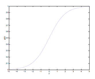
which is the logistic function or sigmoid function

\[g(z) = \frac{1}{1+e^{-z}}\]

which basically:

outputs result between $0,1$
we chose this function specifically because this is actually the special case of the Generalized Linear Model

Useful Properties of Sigmoid Function

Consider the derivative of the function $g$:
\[\begin{align*} g'(z) &= \frac{d}{dz} \frac{1}{1+e^{-z}} \\ &= \frac{1}{(1+e^{-z})^2}(-e^{-z}) \\ &= \frac{1}{1+e^{-z}} \frac{-e^{-z}}{1+e^{-z}} \\ &= \frac{1}{1+e^{-z}}\left( 1 - \frac{1}{1+e^{-z}} \right) \\ &= g(z)\left(1-g(z)\right) \end{align*}\]

Therefore, now we consider the hypothesis:

\[h_\theta(x)=g(\theta^T x)=\frac{1}{1+e^{-\theta^T x}}\]

And the task now is to find out a good cost function.

Heuristics

Recall that for linear regression, we used least squares error which could be derived using the probabilistic model as the maximum likelihood estimator under a set of assumptions, by the following setups:

In the linear regression model, assume the distribution data follows the form of our hypothesis
\[y^{(i)} = \theta^T x^{(i)} + \epsilon^{(i)}\]
where $\epsilon$ is the perturbation which basically introduces the second step

Assuming the perturbation being IID, consider the probability of actually getting $y$ from some $x$:
\[p(y^{(i)} | x^{(i)}; \theta) = \frac{1}{\sqrt{2\pi} \sigma} \exp{\left( - \frac{(y^{(i)} - \theta^T x^{(i)})^2}{2 \sigma^2} \right)}\]

Maximize the probability of $p(y^{(i)}\vert x^{(i)};\theta)$ by optimizing $\theta$, which reaches the conclusion of minimizing:
\[\frac{1}{2}\sum_{i=1}^m (y^{(i)} - \theta^T x^{(i)})^2 = J(\theta)\]
which becomes the error function

Therefore, first we do a similar step of:

Considering a single point, and assume that the distribution of data follows the form of the hypothesis:
\[\begin{align*} P(y = 1 | x;\theta) &= h_\theta (x) \\ P(y = 0 | x; \theta)&= 1 - h_\theta(x) \end{align*}\]
Pictorially

Model: Actual Data:

or compactly, since $y \in {0,1}$:
\[p(y | x; \theta) = (h_\theta(x))^y(1-h_\theta(x))^{1-y}\]
which is also called the Bernoulli Distribution, which has
- the probability mass function being $f(k;\phi) = \phi^k(1-\phi)^{1-k}$ for $k \in {0,1}$
- https://en.wikipedia.org/wiki/Bernoulli_distribution
Assuming that the training samples are generated IID, such that we have the likelihood of parameter/probability of data being given by:
\[\begin{align*} L(\theta) &= p(\vec{y} | X; \theta) \\ &= \prod_{i=1}^m p(y^{(i)}| x^{(i)}; \theta) \\ &= \prod_{i=1}^m (h_\theta(x^{(i)}))^{y^{(i)}}(1-h_\theta(x^{(i)}))^{1-y^{(i)}} \end{align*}\]
Again, to convert the product to easier sums, we consider the log likelihood which is monotonic (i.e. if $f(x)$ increases/decreases, then $\log(f(x))$ also increases/decreases)
\[l(\theta) = \log(L(\theta)) = \sum_{i=0}^m y^{(i)}\log h_\theta(x^{(i)}) + (1-y^{(i)}) \log \left( 1-h_\theta(x^{(i)}) \right)\]
Note
- This function turns out to be a concave function, in other words, there is only one maxima
Now, to maximize the (log) likelihood:
- as compared to the normal equation in linear regression, doing it directly seems non-trivial. It turns out that there is no “normal equation equivalent” for logistic regression
- another “brute-force” away is to consider the (batch) gradient ascent method, where we want to do:
  \[\theta := \theta + \alpha \nabla_\theta l(\theta)\]
  Or written in the form of individual components:
  \[\theta_j := \theta_j + \alpha\frac{\partial}{\partial \theta_j}l(\theta)\]
  Differences against Linear Regression
  - For linear regression, we had batch gradient Descent, which involved: $\theta_j := \theta_j - \alpha\frac{\partial}{\partial \theta_j}J(\theta)$ so we see that the differences are:
    1. the “cost” function is now $l(\theta)$
    2. we are ascending with a plus sign in $+ \frac{\partial}{\partial \theta_j}l(\theta)$, instead of descending with a minus sign in $- \frac{\partial}{\partial \theta_j}J(\theta)$. Even though both are maximizing likelihood

Batch Gradient Ascent Algorithm

Batch Gradient Ascent

The aim is to compute
\[\theta_j := \theta_j + \alpha\frac{\partial}{\partial \theta_j}l(\theta)\]
And below we computed the derivative, so in the end we are computing:
\[\theta_j := \theta_j + \alpha \sum_{i=1}^m (y^{(i)} - h_\theta(x^{(i)})) x^{(i)}_j\]
which again does it by batches (of the entire dataset)

Proof for Derivative of $l(\theta)$:

The gradient ascent algorithm needs the $\frac{\partial}{\partial \theta_j} l(\theta)$ quantity. Like before, we first consider having on one training sample $x^{(1)}$

\[\begin{align*} \frac{\partial}{\partial \theta_j} l(\theta) &= \left( y \frac{1}{g(\theta^T x)} - (1-y)\frac{1}{1-g(\theta^T x)} \right)\frac{\partial}{\partial \theta_j}g(\theta^T x)\\ &= \left( y \frac{1}{g(\theta^T x)} - (1-y)\frac{1}{1-g(\theta^T x)} \right)\left( g'(\theta^Tx) \cdot \frac{\partial}{\partial \theta_j} \theta^T x \right)\\ &= \left( y \frac{1}{g(\theta^T x)} - (1-y)\frac{1}{1-g(\theta^T x)} \right)\left( g(\theta^T x)(1-g(\theta^T x)) \cdot \frac{\partial}{\partial \theta_j} \theta^T x \right)\\ &= \left[ y (1-g(\theta^T x)) - (1-y)g(\theta^Tx)\right] x_j \\ &= (y - h_\theta(x)) x_j \end{align*}\]

where:

obviously $h_\theta(x)=g(\theta^T x)=\frac{1}{1+e^{-\theta^T x}}$
from step 2 to step 3 we used the fact $g’(z) = g(z)(1-g(z))$ from above (property 1 of sigmoid function)

Therefore, for $m$ training samples, we have:

\[\frac{\partial}{\partial \theta_j} l(\theta) = \sum_{i=1}^m (y^{(i)} - h_\theta(x^{(i)})) x^{(i)}_j\]

Perceptron Algorithm

Consider modifying the logistic regression method to be stricter such that it outputs 0 or 1 exactly:

\[g(z) = \begin{cases} 1, & \text{if $z \ge 0$}\\ 0, & \text{if $z < 0$} \end{cases}\]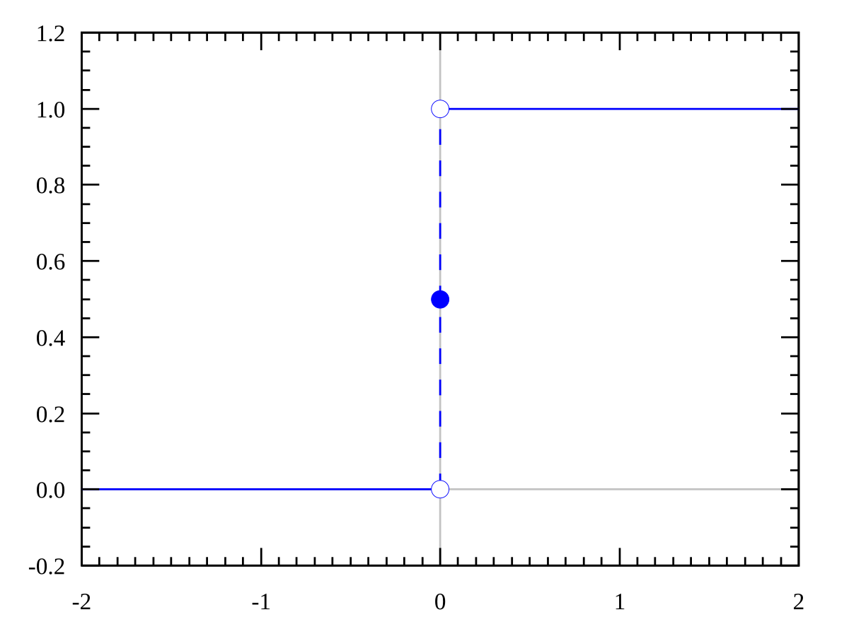

Therefore, we can see this as the stricter version of the sigmoid function:

And more importantly:

Perceptron Algorithm

using this modified definition of $g$, and we use the update rule
\[\theta_j := \theta_j + \alpha (y^{(i)} - h_\theta(x^{(i)})) x^{(i)}_j\]

however, the problem with this is that there turns out to have no obvious probabilistic interpretation of this

Perceptron Algorithm implementation

The perceptron algorithm $\text{Perceptron}(\mathcal{D}_n; \tau)$:

where notice that:

$n$ is the number of data points in your data set

$\tau$ is again a hyperparameter (nothing to do with the logic of algorithm) that you can adjust

$\theta$ is initialized to be a vector in $d$ dimension (same as data points $x$)

$\theta_0$ initialized to be $0$

changed indicates whether if our prediction on each data point is correct or not.

for example, $y^{(i)}\cdot (\theta^T x^{(i)} + \theta_0) \le 0$, if

a data point is not on the line AND current prediction is wrong

a data point is on the line

initial step/loop of iteration

Therefore this actually specifies incorrect prediction of a data point

The part that updates $\theta, \theta_0$ basically does aims to improve $y^{(i)}\cdot (\theta^T x^{(i)} + \theta_0) \le 0$. So that the next iteration looks like:
\[\begin{align*} y^{(i)}\cdot \left((\theta + y^{(i)}x^{(i)})^Tx^{(i)} +(\theta_0 + y^{(i)})\right) &= y^{(i)} (\theta^T x^{(i)} + \theta_0)+(y^{(i)})^2(x^{(i)^T} x^{(i)} + 1)\\ &= y^{(i)} (\theta^T x^{(i)} + \theta_0) + (||x^{(i)}||^2+1) \end{align*}\]
where:

basically we moved the original prediction $y^{(i)} (\theta^T x^{(i)}+\theta_0)$ by some positive value $\vert \vert x^{(i)}\vert \vert ^2+1$

we assumed that $y^{(i)} \in {-1, +1}$ in this case

we return the best line by return the parameter $\theta, \theta_0$

Note

recall first that:

\[\begin{align*} \frac{\theta^T x}{||\theta||} &= -b \\ \theta^T x + b ||\theta|| &= 0\\ \theta^T x + \theta_0 &= 0 \end{align*}\]
so that the more positive the $\theta_0$, the lower/downwards we are moving the line
notice the sign on $\theta_0$ update:
\[\theta_0 = \theta_0 + y^{(i)}\]
this means that if we predicted wrong and that
- $y^{(i)} > 0$, then we need to move the line downwards
- $y^{(i)} < 0$, then we need to move the line upwards
the $\theta$ update:
- rotate the current vector $\theta$ towards the correct/actual result

For Example

Running the above perceptron algorithm would look like:

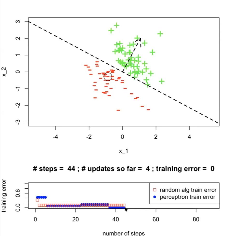
where:

we finished when $t=1, i=44$ (#steps=44)
the “random alg train” in the bottom plot is the $\mathrm{ExLearningAlg}(\mathcal{D}_n;k)$ mentioned before
note that having more steps might increase train error, since
- $\text{ExLearningAlg}(\mathcal{D}_n;k)$ is iterating a step per hypothesis
- $\text{Perceptron}(\mathcal{D}_n; \tau)$ here is iterating over $\tau$ and each point in dataset, and that the adjustment in $\theta, \theta_0$ only moves more towards the current data point

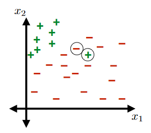
Linearly Separable Dataset

Notice that the above $\text{Perceptron}(\mathcal{D}_n, \tau)$ works if and only if there exists a line that can distinctly separate the binary dataset.

Linearly Separable

A training set $\mathcal{D}_n$ is linearly separable if there exist $\theta, \theta_0$ such that, for every point index $i \in {1,…,n}$, we have:
\[y^{(i)}\cdot (\theta^T x^{(i)} + \theta_0) > 0\]
i.e. correct prediction for all data points

TODO: How do we prove that if a training set is NOT linearly separable?

For Example:

This would not be a linearly separable data set:

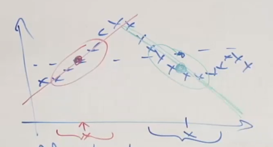
Margin of Training Set

Review:

Consider the signed distance (green part) from a hyperplane defined by $\theta, \theta_0$ to a point $x^*$ below:

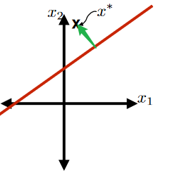
This green part is equivalent to the purple part minus the orange part:

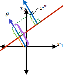
where the
- purple part would be $\frac{\theta^T x^*}{\vert \vert \theta\vert \vert }$
- orange part be $-\frac{\theta_0}{\vert \vert \theta\vert \vert }$
so this is easily:
\[\text{Signed Distance of $x^*$ from Hyperplane}=\frac{\theta^T x^* + \theta_0}{||\theta||}\]

Margin of a Labelled Point

Consider now a labelled point $(x^, y^)$, where $y^{} \in {-1,+1}$. Then the margin of the labelled point $x^, y^*$ with respect to the hyperplane defined by $\theta, \theta_0$ is:
\[\text{Margin of $(x^*, y^*)$}=y^* \left( \frac{\theta^T x^* + \theta_0}{||\theta||} \right)\]
where:

notice the part $\theta^T x^* + \theta_0$ is basically the our prediction of $h(x;\theta, \theta_0)$

$\text{margin}$ of a labelled point would therefore be positive if your hypothesis guessed correctly.

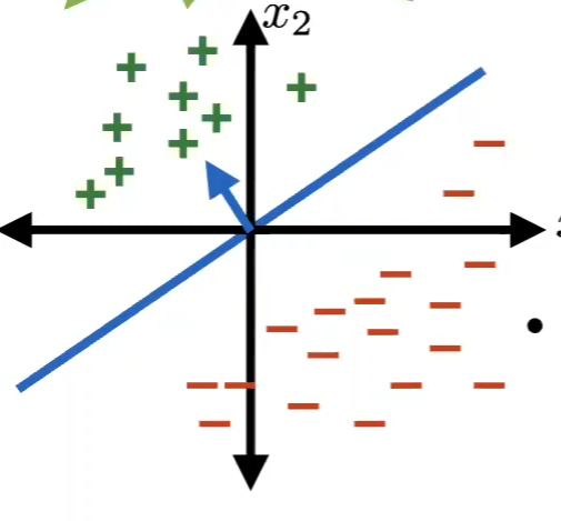
For Example

The hyperplane (blue line) of a specific $\theta, \theta_0$ in the dataset below should have a large margin:

Margin of a Training Set

The margin of a training set $\mathcal{D}_n$ with respect to a hyperplane defined by $\theta, \theta_0$ is:
\[\min_{i \in \{1,...,n\}}y^{(i)}\left(\frac{\theta^T x^* + \theta_0}{||\theta||}\right)\]
where notice that:

if any data point is misclassified, then the margin would be negative

if all data points are classified correctly, then the margin would be positive

The more positive the margin, the easier the classifier is/more separable the dataset

Perceptron Algorithm Performance

Perceptron Performance

The perceptron algorithm will make at most $(R/\gamma)^2$ updates to $\theta$ (i.e. rotate the hyperplane at most $(R/\gamma)^2$ times) util it hits the solution hypothesis, if and only if the following assumptions holds true:

The Hypothesis Class is the set of all linear classifiers with separating hyperplanes that pass through the origin.

this means that $\theta_0=0$ and the hyperplane is completely determined by $\theta$

There exists a $\theta^*$ and $\gamma$ such that $\gamma > 0$ and for every $i \in {1,…,n}$ we have:
\[\text{Margin of $(x^{(i)}, y^{(i)})$}=y^{(i)} \left( \frac{\theta^T x^{(i)} + \theta_0}{||\theta||} \right) > \gamma\]

this means that the dataset is linearly separable

There exists a radius $R$ such that for every $i \in {1,…,n}$, we have $\vert \vert x^{(i)}\vert \vert \le R$

Proof of Assumption 1

Consider a classifier with offset described by $\theta, \theta_0$:

\[x:\theta^Tx + \theta_0 = 0, \quad \text{so that } x\in \mathbb{R}^d,\theta\in \mathbb{R}^d,\theta_0\in \mathbb{R}\]

Then we can convert this equation and eliminate $\theta_0$ by considering:

\[x_\text{new}=[x_1,...,x_d,1]^T, \theta_\text{new}=[\theta_1, ..., \theta_d, \theta_0]^T, \quad \text{so that }x_\text{new} \in \mathbb{R}^{d+1}, \theta_{\text{new}} \in \mathbb{R}^{d+1}\]

Then we have the following being equivalent:

\[\begin{align*} x:\theta^Tx + \theta_0 &= 0 \\ x_{\text{new},1:d}:\theta^T_{\text{new}}x_{\text{new}}&=0 \end{align*}\]

where:

$x_{\text{new},1:d}$ means the first $d$ dimension of the vector $x_\text{new}$
$\theta_0$ has been included in the expanded feature space of $\theta_\text{new}$

Newton’s Method

Comparison against Batch Gradient Ascent

one advantage of this over Batch Gradient Ascent is that it will take less iterations (quadratic convergence) to achieve a good result
one disadvantage is that it is more computationally expensive. See section Higher Dimensional Newton’s Method

Newton’s Method

Task: given a function $f$, the idea is to find $\theta$ such that $f(\theta) = 0$

The idea is to approximate the function near $\theta$ to be a straight line, therefore the next guess of zero is located at:
\[\theta := \theta - \frac{f(\theta)}{f'(\theta)}\]

Usage:

Since we want to maximize $l(\theta)$, we can see it as figuring at $l’(\theta) = 0$ since there is only one global maximum, hence:
\[\theta := \theta - \frac{\ell'(\theta)}{\ell''(\theta)}\]

Proof:

The idea is simple:

where we want to perform the update of:

\[\theta_1 := \theta_0 - \Delta\]

And we know that:

\[\begin{align*} f'(\theta_0) &= \frac{f(\theta_0)}{\Delta}\\ \Delta &= \frac{f(\theta_0)}{f'(\theta_0)}\\ \end{align*}\]

Therefore, we arrive simply at:

\[\theta := \theta - \frac{f(\theta)}{f'(\theta)}\]

Example

Steps	Graphical Illustration
Step 0: given $f$, and a $\theta$ to start with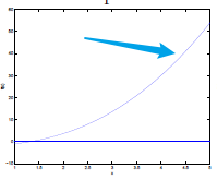
Step 1: Assume that the $f(\theta’)=0$ can be found by going down linearly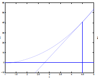
Step 2: Repeat step 1 until $f(\theta’)=0$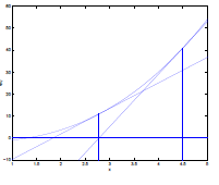

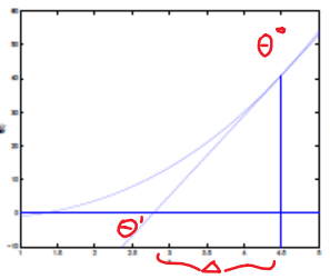
Quadratic Convergence

The idea (informally) is that: if newton’s method on the first iteration has error $0.01$ (away from the true zero), then:

second iteration error=$0.0001$

third iteration error=$0.00000001$

etc.

Higher Dimensional Newton’s Method

Since in some cases we have $\theta$ being a vector in $\mathbb{R}^{n+1}$, then:

Newton’s Method in Higher Dimension

The generalization of Newtons method to this multidimensional setting is:
\[\theta := \theta - H^{-1} \nabla_\theta \ell (\theta)\]
as compared to the one dimensional $\theta := \theta - \frac{1}{\ell’’(\theta)}\ell’(\theta)$, where you now have:

Hessian $H$ being a $\mathbb{R}^{(n+1)\times(n+1)}$ matrix such that
\[H_{ij} = \frac{\partial^2 \ell(\theta)}{\partial \theta_i \partial \theta_j}\]

However, obviously now it becomes computationally difficult to compute $H^{-1}$ if $n+1$ is large for your dataset, i.e. you have lots of features.

Generalized Linear Models

So far, we’ve seen a regression example, and a classification example. In the regression example, we had $y\vert x; \theta ∼ N(\mu, \sigma^2)$, and in the classification one, $y\vert x; \theta ∼ \text{Bernoulli}(\phi)$, for some appropriate definitions of $\mu$ and $\phi$ as functions of $x$ and $\theta$.

In this section, we will show that both of these methods are special cases of a broader family of models, called Generalized Linear Models (GLMs).

Terminologies

Probability Mass Function: distribution for discrete values.
- e.g. Poisson Distribution, Bernoulli Distribution
Probability Density Function (PDF): distribution for continuous values.
- e.g. Normal Distribution

Exponential Family

To work our way up to GLMs, first we need to define the exponential family distributions.

Exponential Family Distribution

We say that a class of distributions is in the exponential family if it can be written in the form:
\[p(y; \eta) = b(y) \exp(\eta \, T(y) - a(\eta))\]
where:

$y$ means the labels/target in your dataset

$\eta$ is the natural parameter (also called the canonical parameter) of the distribution

$b(y)$ is the base measure

$T(y)$ is the sufficient statistic (see later examples, you often see $T(y)=y$)

$a(\eta)$ is the log partition function, which basically has $e^{-a(\eta)}$ playing the role of normalization constant

so basically you can expression some distribution with the above form with any choice of $b(y), T(y), a(\eta)$, then that expression is in the exponential family.

We now show that the Bernoulli and the Gaussian distributions are examples of exponential family distributions.

Example: Bernoulli Distribution

For $y \in {0,1}$, we have the Bernoulli Distribution (recall that we used $h_\theta(x)=\phi$):

\[p(y ; \phi) = \phi^y(1-\phi)^{1-y}\]

We can convert this to the exponential family by:

\[\begin{align*} \phi^y(1-\phi)^{1-y} &= \exp\left( \log(\phi^y(1-\phi)^{1-y}) \right) \\ &= \exp\left(y \log \phi + (1-y)\log (1-\phi)\right)\\ &= 1 \cdot \exp\left( \log\left( \frac{\phi}{1-\phi} \right) y + \log(1-\phi)\right)\\ \end{align*}\]

Therefore, this is in the exponential family with:

$b(y)$ = 1
$T(y) = y$
$\eta = \log\left( \frac{\phi}{1- \phi} \right)$, so that we get $\phi = \frac{1}{1+e^{-\eta}}$
- recall that $\phi = h_\theta(x)$, and that $h_\theta(x)= \frac{1}{1+e^{-\theta^T x}}$ in a similar form!
$a(\eta) = -\log(1-\phi) = \log(1+e^\eta)$

Example: Gaussian/Normal Distribution

For algebraic simplicity, assume that $\sigma^2 = 1$ (recall that when deriving linear regression, the value of $\sigma$ had no effect on our final choice of $\theta$. Therefore, this is also “justified”)

Then we have:

\[p(y; \mu) = \frac{1}{\sqrt{2 \pi}} \exp\left( - \frac{(y-\mu)^2}{2} \right)\]

and doing a similar step as above:

\[\begin{align*} \frac{1}{\sqrt{2 \pi}} \exp\left( - \frac{(y-\mu)^2}{2} \right) &= \frac{1}{\sqrt{2 \pi}} e^{-y^2/2} \cdot \exp\left( \mu y - \frac{1}{2}\mu^2 \right) \end{align*}\]

where now this is matched easily:

$b(y) = \frac{1}{\sqrt{2 \pi}} e^{-y^2/2}$
$T(y) = y$
$\eta = \mu$ which is the natural parameter
$a(\eta) = \mu^2/2 = \eta^2/2$

Properties of Exponential Family

We use the GLM because they have some very nice properties:

Maximum Likelihood Estimate (MLE) with respect to $\eta$ is concave, and the Negative Log Likelihood (NLL) with respect to $\eta$ is convex
The expected value $E[y; \eta] = \frac{\partial}{\partial \eta} a(\eta)$
The variance $\text{Var}[y;\eta] = \frac{\partial^2}{\partial \eta^2} a(\eta)$

Note that the expected value and the variance do not involve integrals now.

Constructing the GLMs

More generally, consider a classification or regression problem where we would like to predict the value of some random variable $y$ as a function of $x$.

e.g. you would like to build a model to estimate the number $y$ of customers arriving in your store (or number of page-views on your website) in any given hour, based on certain features $x$ such as store promotions, recent advertising, weather, day-of-week, etc. (you might think about Poisson Distribution, but that is also a GLM)

To derive a GLM for a problem, we will make the following three assumptions about the conditional distribution of $y$ given $x$ and about our model:

The distribution is in the exponential family, such that $y\vert x;\theta \sim \text{Exponential Family}(\eta)$
The goal is to predict $T(y)$, (in most of the time, $T(y)=y$), so we want to compute $h(x)$. But that $h(x)$ needs to be $h_\theta(x)=E[y\vert x;\theta]$
The natural parameter $\eta$ and inputs $x$ are related linearly, so that $\eta = \theta^T x$. (if $\eta$ is a vector, $\eta_i = \theta^T_i x$)

Pictorially, you think of the following:

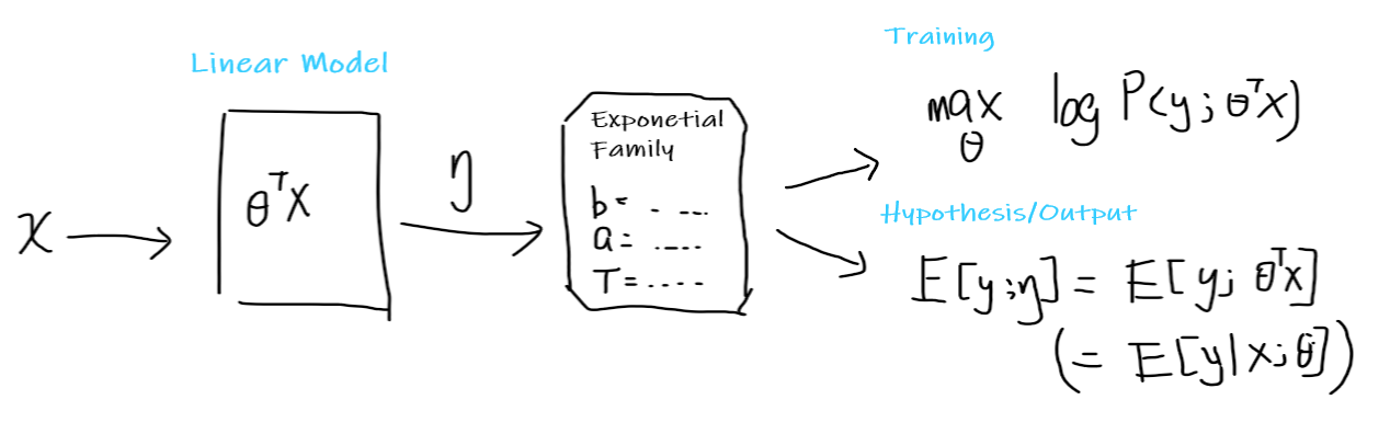
where:

you start with some input $x$
you assume that it is a linear model, so that there exists some learnable parameter $\theta$
- this is the most important assumption here
you convert your input to $\theta^Tx = \eta$
$\eta$ now will give some distribution in the exponential family, by then choosing some appropriate $b(y),a(\eta), T(y)$
- basically your task will give you some hint on what distribution to choose. e.g. modelling website clicks/counts -> use Poisson Distribution, etc.
Using the exponential family:
- your hypothesis function is then simply $h_\theta(x) = E[y;\eta] = E[y;\theta^Tx]=E[y\vert x;\theta]$
- you want to train it to find $\theta$ by maximize likelihood, using the learning update rule
  \[\theta_j := \theta_j + \alpha (y^{(i)} - h_\theta(x^{(i)})) x^{(i)}_j\]
  note that this holds for any distribution in exponential family (or you could use the Batch Gradient Descent, which adds a summation, or the Newton’s Method that we covered above)

Basically, if you your data can be modelled by some distribution in the Exponential Family, you can use GLM above and do the learning.

Terminologies

$\mu = E[y; \eta]= g(\eta)$ is called the canonical response function
- recall that $g(\eta) = \frac{\partial}{\partial \eta} a(\eta)$
$\eta = g^{-1}(\mu)$ is called the canonical link function
Here, we have three types of parameters involved in the GLM,:
- model parameter $\theta$, which we learn in model
- natural parameter $\eta$, which is assumed $\eta = \theta^T x$ to be linear
- canonical parameter, $\phi$ for Bernoulli, $\mu,\sigma$ for Gaussian, $\lambda$ for Poisson, …
  - use $g(\eta)$ to get those canonical parameters from natural parameter
  - use $g^{-1}$ to swap back to natural parameter from canonical parameter

Linear Regression as GLM

Recall that we assumed in Linear Regression:

Model:	Actual Data:

where we model the conditional distribution of $y$ given x as as a Gaussian $N(\mu, \sigma^2)$.

Since we have proven that the Gaussian is in Exponential Family, and that we have proven:

$\mu = \eta$

Therefore, we get from the second assumption in Constructing the GLMs:

\[\begin{align*} h_\theta(x) &= E[y|x; \theta]\\ &= \mu\\ &= \eta \\ &= \theta^T x \end{align*}\]

where we get back the linear hypothesis:

the second equality comes from the fact that $y\vert x;\theta \sim \mathcal{N}(\mu, \sigma^2)$
the last equality comes from the third assumption in Constructing the GLMs:

Logistic Regression as GLM

Recall that for logistic regression:

Pictorially

Model:	Actual Data:

where we model the conditional distribution of $y$ given x as as the Bernoulli Distribution $y\vert x;\theta \sim \text{Bernoulli}(\phi)$.

Since we have also proven that Bernoulli Distribution is in the Exponential Family, and that:

$\phi = 1/(1+e^{-\eta})$

Following a similar derivation from above:

\[\begin{align*} h_\theta(x) &= E[y|x; \theta]\\ &= \phi\\ &= 1/(1+e^{-\eta}) \\ &= 1/(1+e^{-\theta^T x}) \end{align*}\]

which gives back the hypothesis for logistic regression.

once we assume that $y$ conditioned on $x$ is Bernoulli, the sigmoid function arises as a consequence of the definition of GLMs and exponential family distributions.

Softmax Regression

Here we cover the cross entropy interpretation of this method. For the graphical method please refer to the note.

Consider the case when we have to classify more than one class

Then we consider the following representation of this task:

we have $k$ classes
input $x^{(i)} \in \mathbb{R}^n$
label $y$ is a one hot vector, such that $y={0,1}^k$
- e.g. if there are 3 classes, then being in class 1 means $y=[1,0,0]^T$
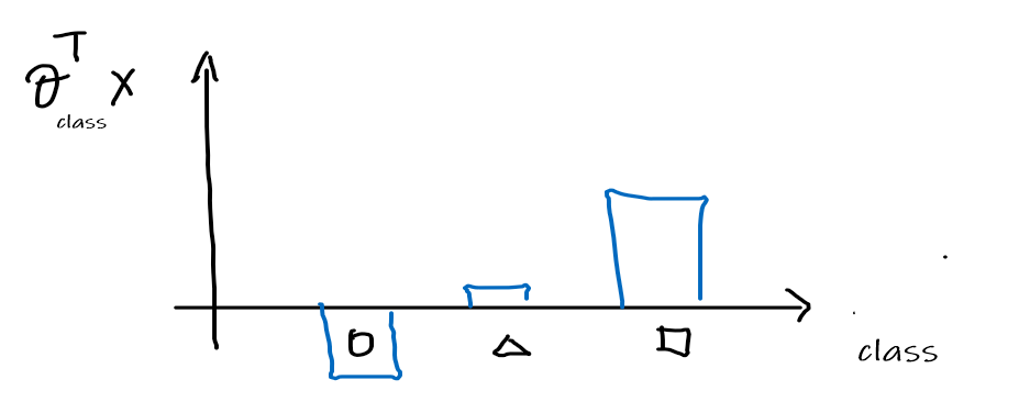
each class has its own parameter $\theta_1,\theta_2,…,\theta_k$, or basically $\phi_1, \phi_2, … \phi_k$ (since $\phi = \theta^T x$)
- technically we only need $k-1$ of those parameters, since it must be that $\sum_{i=1}^k \phi_i = 1$

Then the idea is as follows:

Consider that we have already solved the $\theta_1$ for triangle class, $\theta_2$ for square class, etc

where:
- recall that $\theta^T x \mapsto 1/(1+e^{-\theta^Tx})$, which basically gives the probability of being in the class or not
  - i.e. $\theta^Tx > 0$ means being in the class
Then this means that for any given $x$, we can get compute the $\theta_{\text{class}}^T x$:
Then we can convert this to distribution like values by first making them all positive, applying $\exp$
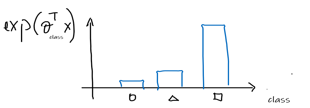
Normalize the distribution to be a probability distribution

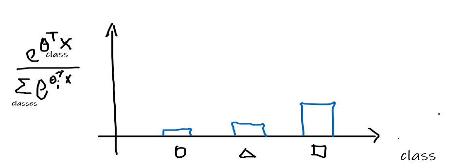
Therefore, this means that given an input $x$, we are outputting a probability distribution
Now, suppose that the actual answer for that $x$ is a triangle, so that $[0,1,0]^T$ is the correct answer. We can convert the answer/label into a distribution as:

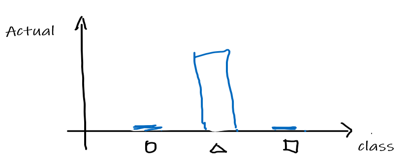
Therefore, then the task/learning algorithm needs to minimize the "difference/distance"=cross entropy between the following two:

Current Model Target

and then output the optimal $\theta_i$ for each class

Therefore, then we need to define:

Cross Entropy

The cross entropy between a prediction $\hat{y}$ and the actual class $y \in {\text{classes}}$
\[\begin{align*} \text{Cross Entropy}(p,\hat{p}|x) &= -\sum_{y \in \text{classes}}p(y) \log \hat{p}(y) \\ &= -\log \hat{p}(y_{\text{correct class}}) \\ &= -\log \frac{e^{\theta_{\text{correct class}}^T x}}{\sum_{i \in \text{classes}}e^{\theta_i^T x}} \end{align*}\]
where:

notice that iff we guessed it right, then this quantity will be zero

otherwise, this will be positive due to the $-$ sign

Our goal is to minimize this quantity, and then we just use gradient descent

Generative Learning Algorithms

Algorithms that try to learn $p(y\vert x)$ directly (such as logistic regression), or algorithms that try to learn mappings directly from the space of inputs $X$ to the labels ${0, 1}$, (such as the perceptron algorithm) are called discriminative learning algorithms. Here, we’ll talk about algorithms that instead try to model $p(x\vert y)$ (and $p(y)$). These algorithms are called generative learning algorithms.

for example, consider the case of classifying between elephants $y=1$ and dogs $y=0$ . A discriminative algorithm would learn the mapping from input features to the animals. A different approach is to build a feature model for each class, which is called the generative learning algorithm

The idea is as follows. If we know $p(x\vert y)$ and $p(y)$, then we can use Bayes’ Rule:

\[p(y|x) = \frac{p(x|y)p(y)}{p(x)} = \frac{p(x|y)p(y)}{p(x|y=1)p(y=1)+p(x|y=0)p(y=0)}\]

For instance, given an input $x$, the probability of it being an elephant $y=1$ is:

\[p(y=1|x) = \frac{p(x|y=1)p(y=1)}{p(x)}\]

where:

$p(y)$ is called the class priors. Basically the probability of something happening regardless of your “features/condition”
$p(x\vert y)$ is your modelled feature
$p(x)$ basically indicates the probability of this set of feature $x$ occurring at all in your sample space

Gaussian Discriminative Analysis

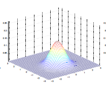
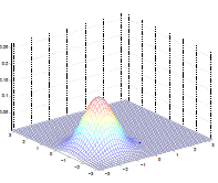
The big assumptions in this model is that $p(x\vert y)$ are distributed as a Gaussian. In other words, if you have many features for $x \in \mathbb{R}^n$ (notice we dropped $x_0=1$ since we are now learning $x$ from $y$), then we assume that $p(x\vert y)$ is distributed as a Multivariate Gaussian.

The Multivariate Normal Distribution

This is basically converting the 1-D Gaussian into something like this:

Multivariable Normal Distribution

This distribution $\mathcal{N}(\mu, \Sigma)$ is parametrized by a mean vector $\mu \in \mathbb{R}^n$ and a covariance matrix $\Sigma \in \mathbb{R}^{n \times n}$, where $\Sigma \ge 0$ and is symmetric and positive semi-definite.

The density function is then given by:
\[p(x;\mu, \Sigma) = \frac{1}{(2\pi)^{n/2} |\Sigma|^{1/2}} \exp\left( -\frac{1}{2}(x-\mu)^T \Sigma^{-1}(x-\mu) \right)\]
where obviously now $x \in \mathbb{R}^n$ is a vector, and that:

$\vert \Sigma\vert$ is the discriminant of $\Sigma$

The mean of a random variable $X \sim \mathcal{N}(\mu, \Sigma)$ is given by:
\[E[X] = \int_x x \,p(x;\mu, \Sigma)dx = \mu\]

The covariance of a vector-valued random variable $Z$ is defined as $\text{Cov}(Z)$:
\[\text{Cov}(Z) = E[\,(Z-E[Z])(Z-E[Z])^T\,] = E[ZZ^T] - (E[Z])(E[Z])^T = \Sigma\]

Examples:

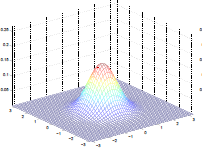
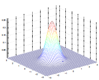
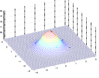
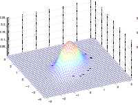
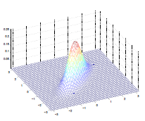
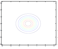
The by varying the covariance $\Sigma$, we could:

$\Sigma=\begin{bmatrix} 1& 0 \ 0 & 1\end{bmatrix}$	$\Sigma=\begin{bmatrix} 0.6& 0 \ 0 & 0.6\end{bmatrix}$	$\Sigma=\begin{bmatrix} 2& 0 \ 0 & 2\end{bmatrix}$

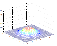which makes sense because:

as covariance $\Sigma \to 0.6\Sigma$, the variation becomes smaller and hence a higher peak
as covariance $\Sigma \to 2\Sigma$, the variation becomes larger and hence a more spread out shape

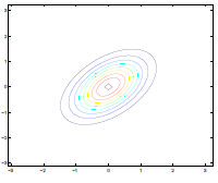
Additionally, we could have non-zero terms to off-diagonal entries

$\Sigma=\begin{bmatrix} 1& 0 \ 0 & 1\end{bmatrix}$	$\Sigma=\begin{bmatrix} 1& 0.5 \ 0.5 & 1\end{bmatrix}$	$\Sigma=\begin{bmatrix} 1& 0.8 \ 0.8 & 1\end{bmatrix}$

where we basically see that:

increasing off-diagonal entries makes the shape more compressed along $x_1=x_2$ $\to$ increases the positive correlation between $x_1, x_2$
technically bottom left contour plots should be circles. Due to aspect ratio problems, they are rendered as ellipses

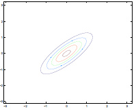
On the contrary, having negative entries creates puts $x_1, x_2$ to have negative correlation

$\Sigma=\begin{bmatrix} 1& 0 \ 0 & 1\end{bmatrix}$	$\Sigma=\begin{bmatrix} 1& -0.8 \ -0.8 & 1\end{bmatrix}$

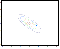Lastly, varying $\mu$ basically shifts the distribution

$\mu = \begin{bmatrix}1\0\end{bmatrix}$	$\mu = \begin{bmatrix}-0.5\0\end{bmatrix}$	$\mu = \begin{bmatrix}-1\-1.5\end{bmatrix}$

The Gaussian Discriminative Analysis Model

Consider the case when we have classification for benign tumors $y=0$ and malignant tumors $y=1$ based on a set of features $x$.

Then if the input features are continuous variables, we start by assuming the following distribution:

\[\begin{align*} y &\sim \text{Bernoulli}(\phi) \\ x|y =0 &\sim \mathcal{N}(\mu_0, \Sigma) \\ x|y =1 &\sim \mathcal{N}(\mu_1, \Sigma) \end{align*}\]

or equivalently:

\[\begin{align*} p(y) &= \phi^y (1-\phi)^{1-y} \\ p(x|y=0) &= \frac{1}{(2\pi)^{n/2} |\Sigma|^{1/2}} \exp\left( -\frac{1}{2}(x-\mu_0)^T \Sigma^{-1}(x-\mu_0) \right) \\ p(x|y=1) &= \frac{1}{(2\pi)^{n/2} |\Sigma|^{1/2}} \exp\left( -\frac{1}{2}(x-\mu_1)^T \Sigma^{-1}(x-\mu_1) \right) \\ \end{align*}\]

where notice that the parameters of the models are:

$\phi, \Sigma, \mu_0, \mu_1$, so that they share the same covariance matrix
- this is assumed that $\Sigma_0=\Sigma_1=\Sigma$, which is usually done, but it does not have to be.

Therefore, given a training set ${(x^{(i)}, (y^{(i)})}_{i=1}^m$, we consider maximizing the (log) Joint Likelihood

\[\begin{align*} L(\phi, \Sigma, \mu_0, \mu_1) &= \prod_{i=1}^m p(x^{(i)}, y^{(i)} ; \phi, \mu_0, \mu_1, \Sigma) \\ &= \prod_{i=1}^m p(x^{(i)}|y^{(i)} ; \phi, \mu_0, \mu_1, \Sigma)p(y^{(i)};\Sigma) \end{align*}\]

where notice that:

now we consider $p(x^{(i)}, y^{(i)} ; \phi, \mu_0, \mu_1, \Sigma)$, which is the probability of $x^{(i)}$ AND $y^{(i)}$ happening at the same time, instead of the linear models which maximizes the conditional probability $p(y\vert x)$

GDA Model

Consider the case when we have a classification problem where features $x$ are all continuous values. Then we can consider the following distribution:
\[\begin{align*} y &\sim \text{Bernoulli}(\phi) \\ x|y =0 &\sim \mathcal{N}(\mu_0, \Sigma) \\ x|y =1 &\sim \mathcal{N}(\mu_1, \Sigma) \end{align*}\]
And then maximize the log of the Joint Likelihood
\[\begin{align*} l(\phi, \Sigma, \mu_0, \mu_1) =\log L(\phi, \Sigma, \mu_0, \mu_1) = \log \prod_{i=1}^m p(x^{(i)}|y^{(i)} ; \phi, \mu_0, \mu_1, \Sigma)p(y^{(i)};\Sigma) \end{align*}\]

By maximizing the log Joint Likelihood (taking derivatives and setting it to zero), you will find that:
\[\begin{align*} \phi &= \frac{1}{m} \sum_{i=0}^m y^{(i)} = \frac{1}{m} \sum_{i=0}^m 1\{y^{(i)}=1\} \\ \mu_0 &= \frac{\sum_{i=1}^m 1\{y^{(i)}=0\}x^{(i)}}{\sum_{i=1}^m 1\{y^{(i)}=0\}} \\ \mu_1 &= \frac{\sum_{i=1}^m 1\{y^{(i)}=1\}x^{(i)}}{\sum_{i=1}^m 1\{y^{(i)}=1\}} \\ \Sigma &= \frac{1}{m} \sum_{i=1}^m (x^{(i)} - \mu_{y^{(i)}})(x^{(i)} - \mu_{y^{(i)}})^T \end{align*}\]
where:

the indicator function behaves as $1{\text{true}}=1$, and $1{\text{false}}=0$

the $\phi$ quantity just computes the average number of patients with malignant tumor

the $\mu_0$ computes the mean of all feature vectors $x$ that corresponds to a benign tumor $y=0$

the $\mu_1$ computes the mean of all feature vectors $x$ that corresponds to a malignant tumor $y=1$

the $\Sigma$ computes the covariance of all feature vectors from their corresponding $\mu_{y^{(i)}}$

Therefore, to make a prediction given some $x$, we compute the quantity:
\[\arg\max_y p(y|x) = \arg\max_y \frac{p(x|y)p(y)}{p(x)} = \arg\max_y p(x|y)p(y)\]
where:

since $p(x)$ is a constant given a $x$, in $\arg \max$ it does not matter

Reminder:

$\arg \max$ or $\arg \min$ works as follows:
\[\begin{align*} \min (z-5)^2 &= 0 \\ \arg \min_z (z-5)^2 &= 5 \end{align*}\]
where basically you care about the argument instead of the output

Pictorially, the computation for $\phi, \mu_0, \mu_1, \Sigma$ is doing the following:

where:

$\Sigma$ fits the contours/shapes of the two Gaussian
- made the two Gaussians have contours that are the same shape and orientation
- one outcome is that the decision boundary will be linear
$\mu_0, \mu_1$ shifts the Gaussian to the “best” place
$\phi$ draws the decision boundary
- technically it is unknown already once the Gaussians are in place, i.e. you know which $y$ is more probable given an $x$

GDA and Logistics Regression

First let’s recall what each algorithm does.

Beginning with the data:

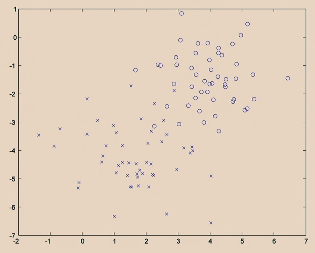
Then logistic regression does:

Iteration 1. initialize randomly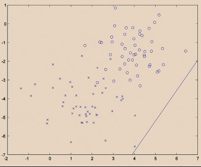
Iteration 2.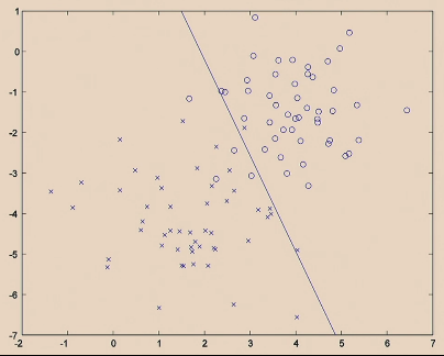
Iteration …
Iteration 20.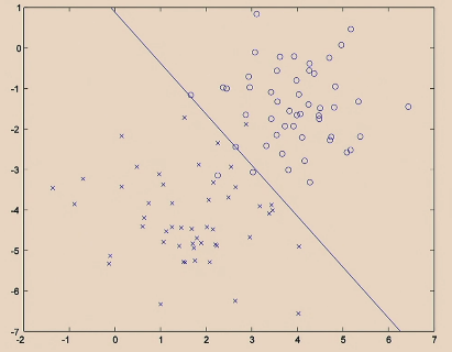

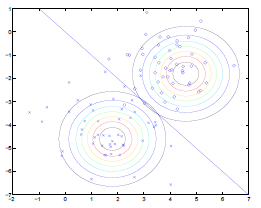
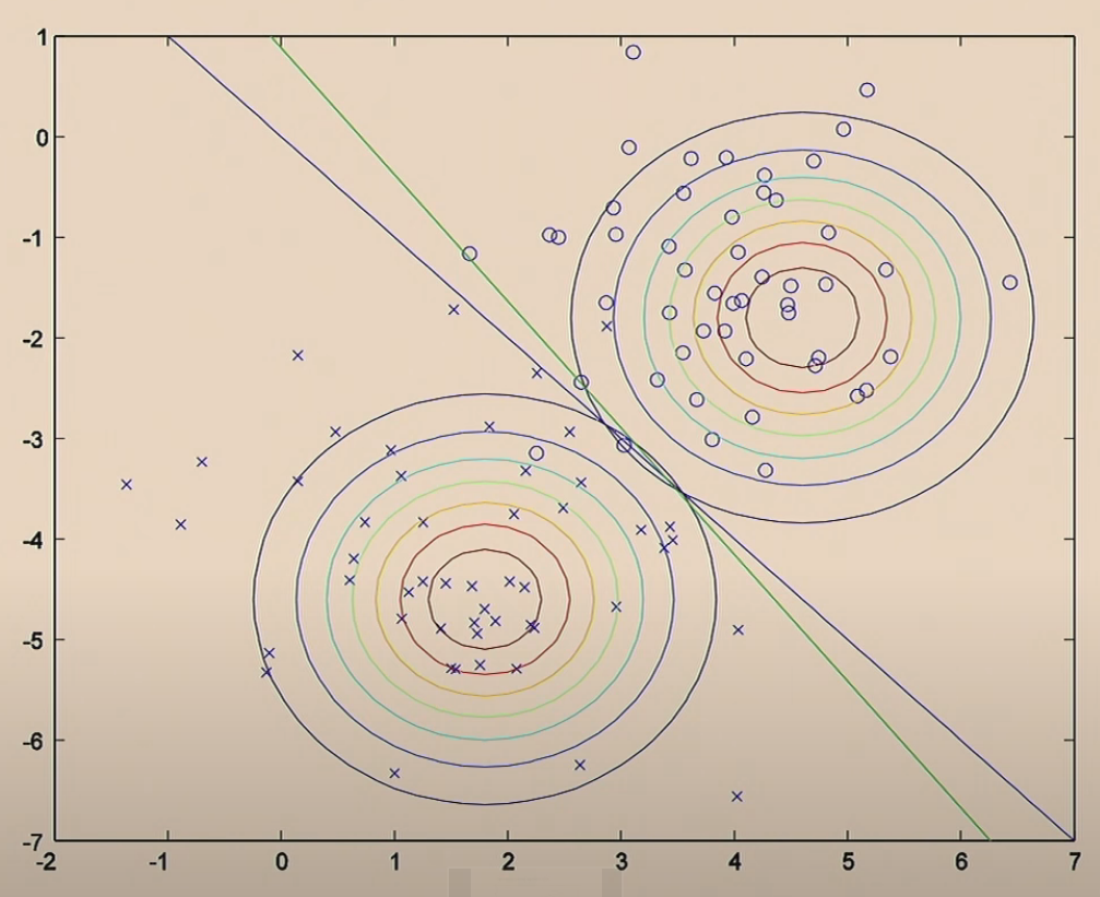
The GDA Model does:

Step 1. Fit Gaussian for each label
Step 2. Decision boundary is implied by the probability for $y$ of each $x$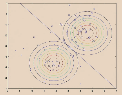

Comparison of the two algorithms:

On the other hand, if we consider the function from GDA, which considers $p(x\vert y)$, and the Bayes Rule:

\[p(y|x) = \frac{p(x|y)p(y)}{p(x)}\]

Consider viewing the quantity $p(y=1\vert x; \Sigma,\mu_0, \mu_1, \phi)$ as a function of $x$, then the following data:

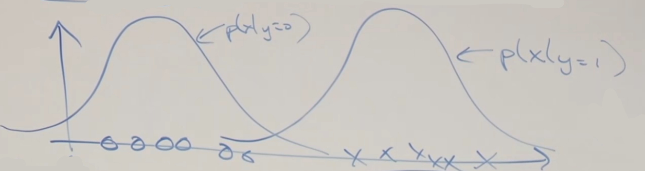
would compute to:

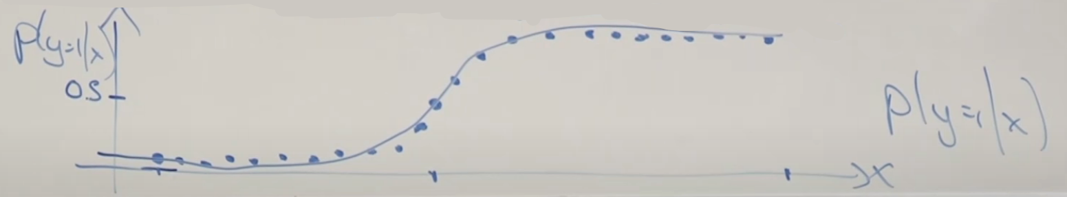
where:

basically points to the left has a very low probability of being $y=1$
points to the far right is almost certainly $y=1$

In fact, it can be proven that this is exactly a sigmoid function

\[p(y=1|x,\phi, \Sigma, \mu_0, \mu_1) = \frac{1}{1+\exp(-\theta^T x)}\]

for $\theta$ being some appropriate function of $\phi, \Sigma, \mu_0, \mu_1$.

Take Away Message

The above basically argues that if $p(x\vert y)$ is multivariate gaussian (with shared $\Sigma$), i.e.
\[\begin{align*} y &\sim \text{Bernoulli}(\phi) \\ x|y =0 &\sim \mathcal{N}(\mu_0, \Sigma) \\ x|y =1 &\sim \mathcal{N}(\mu_1, \Sigma) \end{align*}\]
then $p(y\vert x)$ necessarily follows a logistic function:
\[\begin{align*} p(y=1|x) &= \frac{1}{1+e^{-\theta^T x}}\\ p(y=0|x) &=1- \frac{1}{1+e^{-\theta^T x}} \end{align*}\]
(in fact, this is true for any pair of distributions from the exponential family)

The converse, however, is not true. So in a way the GDA algorithm makes a stronger set of assumptions.

but this means that if assumptions in GDA are correct, then GDA does better than logistic regression since you are telling it more information.

Naïve Bayes

In GDA, the feature vectors $x$ were continuous, real-valued vectors. Let’s now talk about a different learning algorithm in which the $x$’s are discrete valued.

For instance, consider the case of building a email span detector. First you will need to encode text-data into feature vectors. One way to do this is to represent an email by a vector whose length is the number of words in a dictionary:

if an email contains the $i$-th word of the dictionary, then we will set $x_i = 1$. e.g.:

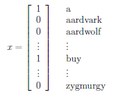
so that $x \in {0,1}^n$

The task is to model $p(x\vert y)$ and $p(y)$ for this generative algorithms.

note that if the size of vocabulary (number of words encoded in the feature vector) is $10,000$, then other models might not work well since you have excessive number of parameters.

Reminder

by the chain rule of probability, we know that:
\[p(x_1, x_2, ...,x_{10,000} | y) = p(x_1|y)\,p(x_2|x_1,y)\,p(x_3|x_1,x_2,y)...p(x_{10,000}|...)\]

Naive Bayes Algorithm

Therefore, in the Naïve Bayes algorithm, we:

assume that $x_i$ are conditionally independent given $y$:
\[p(x_1, x_2, ...,x_{10,000} | y) = p(x_1|y)\,p(x_2|y)\,p(x_3|y)...p(x_{10,000}|y) = \prod_{i=1}^{10000}p(x_i|y)\]
which means that:

given a $y$, e.g. the email being a spam, the chance of the word $\text{buy}$ appearing does not depend on whether if the word $\text{price}$ has appeared in the email (in reality this is usually not true)

This assumption is also called the Naïve Bayes Assumption

then we can consider the following parameters:
\[\begin{align*} \phi_{j|y=1} &= p(x_j=1|y=1) \\ \phi_{j|y=0} &= p(x_j=1|y=0)\\ \phi_y &= p(y=1) \end{align*}\]
where:

$y=1$ represents email being spam

$\phi_y = p(y=1)$ is the class prior

hence the joint likelihood becomes:
\[L(\phi_y, \phi_{j|y=0}, \phi_{j|y=1}) = \prod_{i=1}^m p(x^{(i)},y^{(i)};\phi_y,\phi_{j|y})\]
and solving for the Maximized Likelihood Estimate becomes:
\[\begin{align*} \phi_y &= \frac{\sum_{i=1}^m 1\{y^{(i)}=1\}}{m} \\ \phi_{j|y=1} &= \frac{\sum_{i=1}^m1\{x_j^{(i)}=1 \land y^{(i)}=1\}}{\sum_{i=1}^m1\{y^{(i)}=1\}}\\ \phi_{j|y=0} &= \frac{\sum_{i=1}^m1\{x_j^{(i)}=1 \land y^{(i)}=0\}}{\sum_{i=1}^m1\{y^{(i)}=0\}} \end{align*}\]
where the results are easy to interpret

For instance, $\phi_{j\vert y=1}$ is just the fraction of the spam ($y = 1$) emails in which word $j$ does appear.

Finally, now if we need to compute probability $y=1$ given $x$, we just need to consider:
\[\begin{align*} p(y=1|x) &= \frac{p(x|y=1)\,p(y=1)}{p(x)}\\ &= \frac{\left( \prod_{i=1}^n p(x_i | y=1) \right)p(y=1)}{\left( \prod_{i=1}^n p(x_i | y=1) \right)p(y=1) + \left( \prod_{i=1}^n p(x_i | y=0) \right)p(y=0)} \end{align*}\]

Advantage

this is very fast since there is almost no iterative stuff about it. All it needs to do is to count.

Disadvantage

Naive Bayes assumption is usually not true
A more critical problem is when you get a new word, e.g. NIPS, which corresponds to, say $x_{6017}$. Then you will get:
\[\begin{align*} p(y=1|x) &= \frac{p(x|y=1)\,p(y=1)}{p(x)}\\ &= \frac{\left( \prod_{i=j}^n p(x_j | y=1) \right)p(y=1)}{\left( \prod_{j=1}^n p(x_j | y=1) \right)p(y=1) + \left( \prod_{j=1}^n p(x_j | y=0) \right)p(y=0)}\\ &= \frac{0}{0+0} \end{align*}\]
since $x_{j=6017}$ has never appeared in any past emails, hence $p(x_{6017}\vert y=1) = p(x_{6017}\vert y=0) = 0$

Laplace Smoothing

The idea for this technique is to address the above problem of Naive Bayes, such that having a new sample would not lead to $\frac{0}{0+0}$.

In general, it is statistically a bad idea to estimate the probability of some event to be zero just because you haven’t seen it before in your finite training set.

Consider the case where you have observed your school Football Team’s performance:

Date	Against	Win=1/Lose=0
09/12	AAA	0
09/13	BBB	0
09/14	CCC	0
09/15	DDD	?

where if you think about the probability of the game at 09/15, then your estimate might be:

$p(x=1) = \frac{\text{# Wins}}{\text{# Wins} + \text{# Loses}} = \frac{0}{0+3}=0$

However, this might not be a good idea just because you haven’t seen a win.

Laplace Smoothing

The idea is simple: even if you haven’t seen an event, pretend you did. Therefore, you add $1$ to $\text{# Win}$, and also to all the other cases (to balance out). Therefore, you end up predicting:
\[\frac{(0+1)}{(0+1)+(3+1)}=\frac{1}{5}\]

More generally, if you have $k$ possible outcomes $x \in {1,2,…k}$, then estimating:
\[p(x=j) = \frac{\sum_{i=1}^m 1\{ x^{(i)} = j\} + 1}{m + k}\]

This turns out to be the optimal smoothing if data is distributed uniformly in Bayesian Statistics.

Therefore, applying this to Naïve Bayes

\[\begin{align*} \phi_y &= \frac{\sum_{i=1}^m 1\{y^{(i)}=1\}}{m} \\ \phi_{j|y=1} &= \frac{\sum_{i=1}^m1\{x_j^{(i)}=1 \land y^{(i)}=1\} + 1}{\sum_{i=1}^m1\{y^{(i)}=1\} + 2}\\ \phi_{j|y=0} &= \frac{\sum_{i=1}^m1\{x_j^{(i)}=1 \land y^{(i)}=0\} + 1}{\sum_{i=1}^m1\{y^{(i)}=0\} + 2} \end{align*}\]

and notice that:

\[\sum_{j=1}^{k} \phi_j = 1\]

still holds.

Event Model for Text Classification

Recall that for Naïve Bayes above (also called Multivariate Bernoulli Model):

we first assumed that emails generated are randomly determined to be spam or none spam (according to the class priors $p(y)$)
then we assumed that the words in the emails are also chosen independently according to the probability $p(x_i=1\vert y)=\phi_{i\vert y}$

Another shortcoming for this is that we are only dealing with each word for once, hence ignoring some information which might be useful.

Here. we consider a multinomial event model, which states that:

Let $x_i$ denote the identity of the $i$-th word in the email. This means that an email of $n$ words is now represented by a vector $[x_1, x_2,\dots , x_n]^T$ of length $n$. For instance, if an email starts with “A NIPS . . . ,” then $x_1 = 1$ (“a” is the first word in the dictionary), and $x_2 = 35000$.
- therefore, this means that inputs are of variable size
Then we assume that emails generated are randomly determined to be spam or none spam (according to the class priors $p(y)$)
- this is the same as before
Then we assume that the sender composes the email by first generating $x_1$ from some multinomial distribution over words $p(x_1\vert y)$. Next the second word $x_2$ is chosen independently of $x_1$ but from the same distribution, i.e. $p(x_2\vert y)$.

Therefore, we can say a similar assumption from the Naïve Bayes:

\[\begin{align*} p(x) &= p(x|y)p(y) \\ &= p(y)\prod_{i=1}^n p(x_i | y) \end{align*}\]

This means that we have the following parameters:

\[\begin{align*} \phi_{y} &\equiv p(y=1)\\ \phi_{k|y=1} &\equiv p(x_j=k|y=1)\\ \phi_{k|y=0} &\equiv p(x_j=k|y=0) \end{align*}\]

where:

this looks similar to the Naive Bayes before, but with a different meaning: $p(x_j=k\vert y=0)$ means the chance of the $i$-th word of a message $x$ being the $k$-th word of the dictionary given that the email is not spam ($y=0$)
notice that $\phi_{k\vert y=0} \equiv p(x_j=k\vert y=0)$ has $j$ not appearing on the LHS, we assumed that the chance of $x_1=k$ is the same as $x_2=k$, etc.

Therefore, given a new email $x$, you can compute everything if you know the $\phi_{y}, \phi_{k\vert y=1}, \phi_{k\vert y=0}$, by considering:

\[\begin{align*} p(y=1|x) &= \frac{p(x|y=1)\,p(y=1)}{p(x)}\\ &= \frac{\left( \prod_{i=1}^n p(x_i | y=1) \right)p(y=1)}{\left( \prod_{i=1}^n p(x_i | y=1) \right)p(y=1) + \left( \prod_{i=1}^n p(x_i | y=0) \right)p(y=0)} \end{align*}\]

Multinomial Event Model

Therefore, given the traning set ${(x^{(i)},y^{(i)});i=1,…,m}$ where $x^{(i)}$ is of variable size $(x_1^{(i)},…,x_{n_i}^{(i)})$, then we consider the likelihood of the parameter given the dataset being:
\[\begin{align*} \mathcal{L}(\phi_y,\phi_{k|y=0}, \phi_{k|y=1}) &= \prod_{i=1}^m p(x^{(i)}, y^{(i)})\\ &= \prod_{i=1}^m \left( p(y^{(i)};\phi_y) \prod_j^{n_i} p(x^{(i)}_j|y^{(i)} ; \phi_{k|y=0},\phi_{k|y=1})\right) \end{align*}\]
Maximizing the likelihood estimates we get:
\[\begin{align*} \phi_{k|y=1} &= \frac{\sum_{i=1}^m \sum_{j=1}^{n_i}1\{x_j^{(i)}=k \land y^{(i)} = 1\}}{\sum_i^m 1\{y^{(i)}=1\}n_i}\\ \phi_{k|y=0} &= \frac{\sum_{i=1}^m \sum_{j=1}^{n_i}1\{x_j^{(i)}=k \land y^{(i)} = 0\}}{\sum_i^m 1\{y^{(i)}=0\}n_i}\\ \phi_{y} &= \frac{\sum_{i=1}^m 1\{y^{(i)}=1\} }{m}\\ \end{align*}\]
where basically:

$\phi_{k\vert y=1}$ means the number of word $k$ appearing in all spam email divided by the total number of words in all spam email

other parameters are obvious

Using Laplace Smoothing, if our dictionary is of size $10,000$ words, then:
\[\phi_{k|y=1} = \frac{1+\sum_{i=1}^m \sum_{j=1}^{n_i}1\{x_j^{(i)}=k \land y^{(i)} = 1\}}{10,000 + \sum_i^m 1\{y^{(i)}=1\}n_i}\]
because:

the denominator basically indicates the $p(x_j = k \vert y=1)$, which has $10,000$ possible outcomes since our dictionary is of size $10,000$

in other words, you can think about the case when you have no dataset, then the probability of a new spam email having $j$-th word being $k$ is $p(x_j = k \vert y=1) = 1/10,000$.

Support Vector Machines

One advantage of using SVM is that it can fit nonlinear boundaries

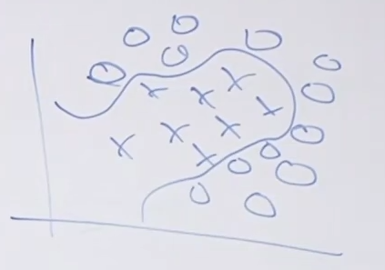
The idea is that this thing can:

take some input features, say two dimensional $[x_1,x_2]$, and map them to some higher dimensional feature $[x_1,x_2,x_1^3,x_2^{-5}]$, etc.
then do a linear classifier on those higher dimensional features

(This model is in general great, not as good as neural networks, but easy to use and quite robust.)

Margins: Intuitions

We’ll start our story on SVMs by talking about margins. In general, there are two ways to think about confidence of a prediction:

Functional Margin
Geometric Margin

Functional Margin Intuition

Consider the case for a logistic regression, where we defined $g(z) = \frac{1}{1+e^{-z}}$ and that $h_\theta(x) = g(\theta^Tx)$. Since the output of this model is between $(0,1)$, then we would want that, for a training sample $x$:
\[\begin{cases} \theta^T x \gg 0, &\text{if $y$ turns out to be $1$}\\ \theta^T x \ll 0, &\text{if $y$ turns out to be $0$} \end{cases}\]
in other words, if $h_\theta(x)$ predicts probability very close to $1$ if $y$ is actually $1$, and vice versa.

This seems to be a nice goal to aim for, and we will soon formalize this idea

Another idea is to think about it geometrically

Geometric Margin Intuition

In a similar case, consider two working hypothesis

where:

the black lines seems to be better than the red line, because points are further away from the decision boundary.

in a sense this idea is similar to the functional margin

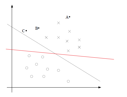
Notations

To make our discussion of SVMs easier, we’ll first need to introduce a new notation for talking about classification.

Labels: $y \in {-1,+1}$ for binary class.
- Therefore, $g(z)=1$ if $z\ge 0$, and $g(z)=-1$ if $z < 0$, where $g$ is the sigmoid function
Hypothesis: $h_{w,b}(x) = g(w^T x + b)$
- now we remove the $x_0=1$ from $x$, and made it to be $b$ explicitly
- therefore, basically $[\theta_0, \theta_1,\dots,\theta_n] \mapsto [b,w_1,\dots,w_n]$

Functional and Geometric Margins

Now we can formalize the idea of functional and geometrical margins.

for this section, we assume that the data is linear separable

Functional Margin

Given a training sample $(x^{(i)},y^{(i)})$, we define the functional margin $\hat{\gamma}$ of parameters $(w,b)$ to be:
\[\hat{\gamma}^{(i)} \equiv y^{(i)}(w^Tx + b)\]
where basically we want to maximize $\hat{\gamma}$ because we want:

when $y^{(i)}=1$, then $(w^Tx + b) \gg 0$

when $y^{(i)}=-1$, then $(w^Tx + b) \ll 0$

and $\hat{\gamma} > 0$ means prediction is correct

Therefore, larger $\hat{\gamma}$ means more confidence and correct prediction

Therefore, the functional margin for a given dataset is defined to be:
\[\hat{\gamma} = \min_{i =1,...,m} \hat{\gamma}^{(i)}\]
where basically we are taking the worst margin.

and assuming that it is linearly separable

Note

You might want to also impose the constraint that $(w,b) \to (w/\vert \vert w\vert \vert , b/\vert \vert w\vert \vert )$ to prevent the case where you can increase $\hat{\gamma}$ by just having $w \to 10w, \, b \to 10b$ without really changing anything (same line equation).

Geometric Margin

Given some training samples $(x^{(i)},y^{(i)})$, we consider the hypothesis:

where for a single data point $A$, the geometric margin is the Euclidean distance of it, line $AB$, from the hyperplane/line

Therefore, we can formalize this to be:
\[\gamma^{(i)} = \frac{w^T x^{(i)} + b}{||w||}\]
where this is for the positive example, which is also proven below.

To be generalized, and notice that $w^T x^{(i)} + b = \hat{\gamma}^{(i)}$ which is the functional margin, we hence get:
\[\gamma^{(i)} = \frac{\hat{\gamma}^{(i)}}{||w||}\]
which clarifies the relationship between the two margins.

Finally, for the entire training set, we have the geometric margin being:
\[\gamma = \min_{i=1,...,m} \gamma^{(i)}\]

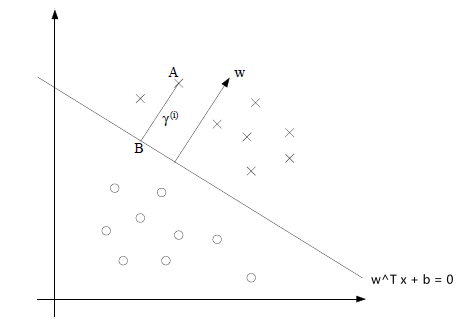
Proof

Consider the point $B$, which lies on the boundary. This point $B$ can be calculated by:

\[x^{(i)} - \gamma^{(i)} \frac{w}{||w||}\]

Since this point lies on the line, this means that:

\[w^T\left( x^{(i)} - \gamma^{(i)} \frac{w}{||w||} \right) + b = 0\]

Therefore, solving for the above yields:

\[\gamma^{(i)} = \frac{w^T x^{(i)} + b}{||w||}\]

The Optimal Margin Classifier

Again, for now we assume that the data is linearly separable.

Now, the sensible idea for a good fit is to find a decision boundary that maximizes the geometric margin.

Mathematically, to maximize it, we can pose the following problem:

\[\begin{align*} \max_{\gamma, w,b} &\quad \gamma\\ \text{s.t.} &\quad y^{(i)}(w^T x^{(i)} + b) \ge \gamma, \quad i=1,...,m\\ &\quad ||w||=1 \end{align*}\]

where:

i.e. we want to maximize $\gamma$, such that each training example has geometric/functional margin of at least $\gamma$.
notice that since $\vert \vert w\vert \vert =1$, functional margin is the same as geometric margin.

However, this turns out to be very difficult to solve since $\vert \vert w\vert \vert =1$ constraint is a non-convex one.

It turns out that the above problem can be rephrased as the following:

\[\begin{align*} \min_{w,b} &\quad \frac{1}{2}||w||^2\\ \text{s.t.} &\quad y^{(i)}(w^T x^{(i)} + b) \ge 1,\quad i=1,...,m \end{align*}\]

whose solution of $w,b$ gives the optimal margin classifier.

Proof

First, we consider moving the $\vert \vert w\vert \vert$ away from the constraint. Recall that $\gamma = \hat{\gamma}/\vert \vert w\vert \vert$:

\[\begin{align*} \max_{\gamma, w,b} &\quad \frac{\hat{\gamma}}{||w||}\\ \text{s.t.} &\quad y^{(i)}(w^T x^{(i)} + b) \ge \hat{\gamma},\quad i=1,...,m \end{align*}\]

which introduced the problem to the $\max$ statement.

Now, recall that scaling $w,b$ has the same as scaling $\hat{\gamma}$ without changing anything. Therefore, we can impose a scaling constraint on $w,b$ w.r.t. the training set such that the functional margin $\hat{\gamma}$ must be 1. Now we can change the problem to forcing $\vert \vert w\vert \vert = 1/ \gamma$. Therefore, the problem becomes:

\[\begin{align*} \max_{\gamma, w,b} &\quad \frac{1}{||w||}\\ \text{s.t.} &\quad y^{(i)}(w^T x^{(i)} + b) \ge 1,\quad i=1,...,m \end{align*}\]

so instead of maximizing $1/

$, you can minimize $$

^2$$. Adding a coefficient to make derivatives easier:

\[\begin{align*} \min_{w,b} &\quad \frac{1}{2}||w||^2\\ \text{s.t.} &\quad y^{(i)}(w^T x^{(i)} + b) \ge 1,\quad i=1,...,m \end{align*}\]

which can be more easily solved, since now you have $w$ becoming a concave function

Now, what if the size of feature is much much greater than we thought? Consider the case that $x \in \mathbb{R}^{10,000}$. To do something with this, we need to assume that the parameter $w$ is some linear combination of data points $x^{(i)}$:

\[w = \sum_{i=1}^m \alpha_i y^{(i)} x^{(i)}\]

where:

$\alpha_i$ is some coefficient $\in \mathbb{R}$
$y^{(i)}$ in the label. In this example we assume $y^{(i)} \in {-1,+1}$
$x^{(i)}$ is the $i$-th input feature

Intuition

This assumption is actually not that absurd. Recall that in (stochastic) gradient descent algorithms that we did, we chose to update $\theta$ by:
\[\begin{align*} \theta &:=\theta - \alpha \left(h_\theta(x^{(i)})-y^{(i)}\right)x^{(i)}\\ \end{align*}\]
since we initialized $\theta = 0$, this is essentially a linear combination of all data points (this is also true for batch gradient descent).

The graphical idea is that your $w$ should always be in the span of $x^{(i)}$, i.e. $\text{Span}{x^{(1)}, …, x^{(m)}}$

For example, if you have three features yet they only lie in a 2D space, then:

where notice that your $w$ hence should be in the $\text{Span}{x^{(1)}, …, x^{(m)}}$

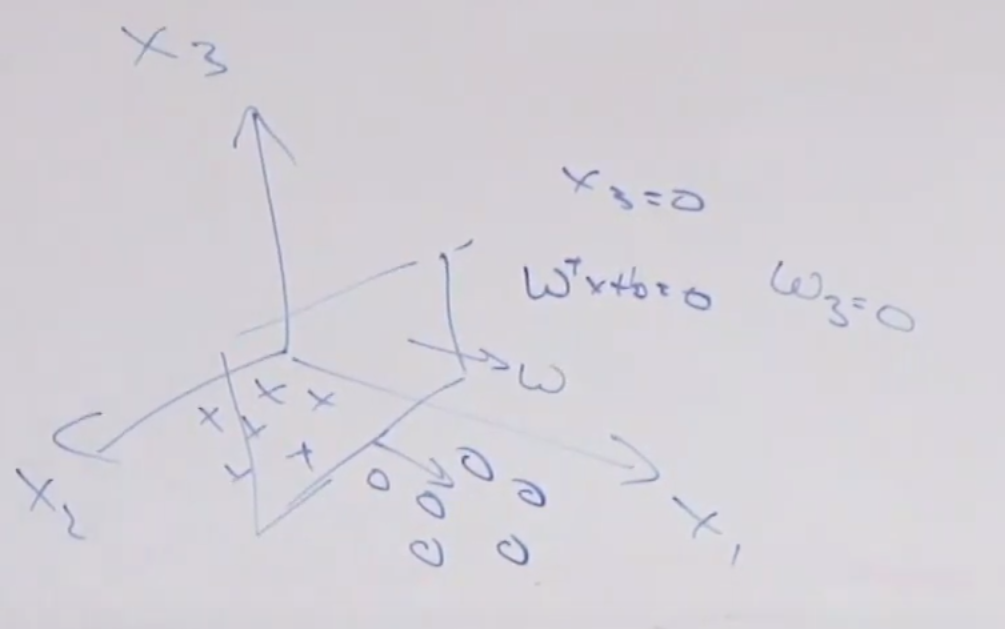
The formal proof of this is called the representor theorem, which is much more complicated than needed here.

Therefore, by plugging in the new assumption, we can then rewrite the optimal margin problem to be:

\[\begin{align*} \min_{w,b} &\quad \frac{1}{2}\left( \sum_{i=1}^m \alpha_i y^{(i)} x^{(i)}\right)^T \left( \sum_{i=1}^m \alpha_i y^{(i)} x^{(i)}\right)\\ \text{s.t.} &\quad y^{(i)}\left(\left( \sum_{i=1}^m \alpha_i y^{(i)} x^{(i)}\right)^T x^{(i)} + b\right) \ge 1,\quad i=1,...,m \end{align*}\]

using the (almost) braket notation (recall from quantum mechanics), which states $\langle{x^{(i)}},{x^{(i)}}\rangle=x^{(i)^T}x^{(i)}$, we then have:

\[\begin{align*} \min_{\alpha} &\quad \frac{1}{2}\sum_{i=1}^m \sum_{j=1}^m \alpha_i \alpha_jy^{(i)}y^{(j)} \lang x^{(i)},x^{(j)} \rang \\ \text{s.t.} &\quad y^{(i)}\left(\sum_{i=1}^m \alpha_i y^{(i)} \lang x^{(i)},x^{(i)} \rang + b\right) \ge 1,\quad i=1,...,m \end{align*}\]

notice that:

here the parts that relates to the input is the inner product $\lang x^{(i)},x^{(j)} \rang$. Therefore, if we could somehow compute this part efficiently, then we would be able to compute this even if features are in infinite dimension.
the only parameter now is $\alpha$ instead of $w, b$

Lastly, you can further simplify this optimization problem using Lagrange Duality:

\[\begin{align*} \max_{\alpha} &\quad \sum_{i=1}^m \alpha_i - \frac{1}{2} \sum_{i,j=1}^m \alpha_i \alpha_jy^{(i)}y^{(j)} \lang x^{(i)},x^{(j)} \rang\\ \text{s.t.} &\quad \alpha_i \ge 0,\, i=1,...,m\\ &\quad \sum_{i=1}^m \alpha_i y^{(i)} = 0 \end{align*}\]

after we found the optimal parameter $\alpha$, we can then compute back the original, optimal parameters $w^,b^$ by:

\[w^* = \sum_{i=1}^m \alpha_i y^{(i)}x^{(i)}\] \[b^* = -\frac{ \max_{i:y^{(i)}=-1} w^{*^T}x^{(i)} + \min_{i:y^{(i)}=1}w^{*^T}x^{(i)}}{2}\]

where notice that the first equation was the "assumption" we made that the **parameter $w$** is some linear combination of data points $x^{(i)}$. (To see the whole proof, see section Lagrange Duality)

Optimal Margin Classifier

The problem is that to maximize $\gamma$ by figuring out parameters $w,b$. It turns out that the above problem can be rephrased as the following:
\[\begin{align*} \min_{w,b} &\quad \frac{1}{2}||w||^2\\ \text{s.t.} &\quad y^{(i)}(w^T x^{(i)} + b) \ge 1,\quad i=1,...,m \end{align*}\]
which can be then converted to solving for $\alpha$:
\[\begin{align*} \max_{\alpha} &\quad \sum_{i=1}^m \alpha_i - \frac{1}{2} \sum_{i,j=1}^m \alpha_i \alpha_jy^{(i)}y^{(j)} \lang x^{(i)},x^{(j)} \rang\\ \text{s.t.} &\quad \alpha_i \ge 0,\, i=1,...,m\\ &\quad \sum_{i=1}^m \alpha_i y^{(i)} = 0 \end{align*}\]
where the optimal value of $\alpha$ can then be used to solve back the parameters $w, b$ by:
\[\begin{align*} w^* &= \sum_{i=1}^m \alpha_i y^{(i)}x^{(i)} \\ b^* &= -\frac{ \max_{i:y^{(i)}=-1} w^{*^T}x^{(i)} + \min_{i:y^{(i)}=1}w^{*^T}x^{(i)}}{2} \end{align*}\]
whose solution of $w,b$ gives the optimal margin classifier.

Then, to make a prediction when a new input $x$ comes in:
\[h_{w,b}(x) = g(w^Tx+b)\]
where since $g(z)$ is the sigmoid function, we basically predicts class-1 iff $w^Tx+b > 0$. Hence this becomes computing the quantity:
\[\begin{align*} w^Tx + b &= \left( \sum_{i=1}^m \alpha_i y^{(i)}x^{(i)} \right)^T x + b \\ &= \sum_{i=1}^m \alpha_i y^{(i)}\lang x^{(i)},x \rang + b \end{align*}\]
which:

basically only needs to compute the inner product between an input $x$ against all data points $x^{(i)}$

Lagrange Duality

First lets us do some reviews on gradient vector and Lagrange multiplier

Review: Gradient Vector

For some intuition, consider a function $F$ takes some point/vector in 3-dimension. So $F:\mathbb{R^3} \to \mathbb{R}$ is a function of three variables.

Now, by definition, the total derivative of $F$ at a point $p \in \mathbb{R^3}$ is the best linear approximation near $p=(a,b,c)$:

\[\left.dF\right|_{p}(\Delta x, \Delta y, \Delta z) = \left.\frac{\partial F}{\partial x}\right|_p\Delta x + \left.\frac{\partial F}{\partial y}\right|_p\Delta y + \left.\frac{\partial F}{\partial z}\right|_p\Delta z\]

Additionally:

\[\left.dF\right|_{p}(\Delta x, \Delta y, \Delta z) + F(p) \approx F(a+\Delta x, b+\Delta y, c+\Delta z)\]

Therefore, the total derivative can be understood as:

\[\left.dF\right|_{p}(\Delta x, \Delta y, \Delta z) = \lang \left.\frac{\partial F}{\partial x}\right|_p, \left.\frac{\partial F}{\partial y}\right|_p, \left.\frac{\partial F}{\partial z}\right|_p \rang \cdot \lang \Delta x, \Delta y, \Delta z \rang\]

Therefore, we can define gradient vector at $p$ to be $\nabla F\vert _p = \lang \left.\frac{\partial F}{\partial x}\right\vert _p, \left.\frac{\partial F}{\partial y}\right\vert _p, \left.\frac{\partial F}{\partial z}\right\vert _p \rang$. Since $p$ can be any point, we get that in general:

\[\nabla F = \lang \frac{\partial F}{\partial x}, \frac{\partial F}{\partial y}, \frac{\partial F}{\partial z}\rang\]

and hence, the total derivative is the DOT PRODUCT of:

\[dF|_p (\vec{\mathrm{v}}) = \nabla F|_p \cdot \vec{\mathrm{v}}\]

In words, to see how much $F(p)$ changes when you move away a little bit from $\vec{p}$ to $\vec{p} + \vec{v}$ for some unit vector $\vec{v}$ just dot product $\nabla F\vert _p \cdot \vec{\mathrm{v}}$.

Therefore, it is easy to see that if you have a level curve, $F(\vec{x})=0$, then gradient vector of a level curve is perpendicular to the level curve.

Review: Lagrange Multiplier

Consider finding local maxima/minima of a multivariate function $f(\vec{x})\mapsto \mathbb{R}$ subject to some constraint $g(\vec{x}) = 0$.

Since the constraint is basically a level curve, local maxima/minima points $\vec{x}$ on the level curve must satisfy:

\[\nabla{f} = - \lambda \nabla g\]

for some constant multiplier $\lambda$ which is also called the Lagrange Multiplier.

Now, what if you have inequality constraint, for example $g(\vec{x}) \le 1$? Then one intuitive approach would be:

First we can look at the area within the region. Compute the normal optimization problem of $f(\vec{x})$, and then see if there are maxima/minima within $g(\vec{x}) < 1$.
Then we compute the optimization problem on the boundary $g(\vec{x}) = 1$.
Lastly, we look at the corners of the boundary if there are.
- the absolute maxima on the boundary are either local optima on the boundary, or absolute optima at the corner of the boundary
Now we just compare the values of the points found, and pick the larges/smallest if you are finding maxima/minima.

Resources

https://math.stackexchange.com/questions/49473/lagrange-multipliers-with-inequality-constraints-minimize-f-on-the-region-0

https://users.wpi.edu/~pwdavis/Courses/MA1024B10/1024_Lagrange_multipliers.pdf

another method

Now, coming back to the topic. Consider some constraint optimization problem:

\[\begin{align*} \min_w &\quad f(w)\\ \mathrm{s.t.} &\quad h_{i}(w)=0,\,\,\,\, i=1,...,l \end{align*}\]

Though such problems can be solved using Lagrange Multipliers, here we consider another related approach. Define the Lagrangian to be:

\[\mathcal{L}(w, \beta) = f(w) + \sum_{i=1}^l \beta_i h_i(w)\]

where now $\beta_i$ are the Lagrange multipliers. Then using the fact from Lagrange Multiplier that $\nabla f = -\beta_i \nabla h_i$, the optimization problem becomes solving:

\[\frac{\partial \mathcal{L}}{\partial w_i} = 0; \quad \frac{\partial \mathcal{L}}{\partial \beta_i} = 0;\]

which then you need to solve for $w, \beta$.

In this section, we will generalize this to constrained optimization problems in which we may have inequality as well as equality constraints.

First, consider the primal optimization problem:

\[\begin{align*} \min_w &\quad f(w)\\ \mathrm{s.t.} &\quad g_i(w) \le 0, \,\, i=1,...,k \\ &\quad h_i(w) = 0, \,\, i=1,...,l \end{align*}\]

Then we have the generalized Lagrangian:

\[\mathcal{L}(w, \alpha, \beta) = f(w) + \sum_{i=1}^k\alpha_i g_i(w)+ \sum_{i=1}^l \beta_i h_i(w)\]

where $\alpha_i, \beta_i$ are the Lagrange multipliers.

Primal Problem

Consider the primal optimization problem above. We consider the quantity:
\[\theta_\mathcal{P}(w) = \max_{\alpha,\beta ; \alpha_i \ge 0} \mathcal{L}(w,\alpha, \beta)\]
where the $\mathcal{P}$ stands for primal. Then we know that:
\[\theta_{\mathcal{P}}(w) = \begin{cases} f(w) &\text{if $w$ satisfies primal constraints} \\ \infty &\text{otherwise} \end{cases}\]
where this is easy to see since, if some $w$ violates the primal constraints that either $g_i(w) > 0$ or $h_i(w) \neq 0$, then notice that:
\[\begin{align*} \theta_{\mathcal{P}} &= \max_{\alpha, \beta: \alpha_i \ge 0} f(w) + \sum_{i=1}^k \alpha_i g_i(w) + \sum_{i=1}^l \beta_ih_i(w) \\ &= \infty \end{align*}\]
because either $g_i(w)$ term could explode to infinity or $h_i(w)$ term would explode.

Therefore, the primal problem can be rephrased as:
\[\min_w \theta_{\mathcal{P}}(w) = \min_w \,\, \max_{\alpha,\beta:\alpha_i \ge 0} \mathcal{L}(w, \alpha, \beta)\]

For later use, let us define the optimal value/solution of the above problem be $p^* = \min_w \theta_{\mathcal{P}}(w)$. This value will be referred to as the value of the primal problem

Now let us consider a slightly different problem, which is:

\[\theta_\mathcal{D}(\alpha, \beta) = \min_w \mathcal{L}(w,\alpha, \beta)\]

where $\mathcal{D}$ stands for dual.

Dual Optimization Problem

Using the above definition, we can pose another (related but not directly related) problem:
\[\max_{\alpha,\beta : \alpha_i \ge 0} \theta_\mathcal{D}(\alpha, \beta) = \max_{\alpha,\beta : \alpha_i \ge 0} \min_w \mathcal{L}(w,\alpha, \beta)\]
which is the same primal optimization problem but $\min$ and $\max$ are reversed.

Similarly, we can define the value $d^*=\max_{\alpha,\beta : \alpha_i \ge 0} \theta_\mathcal{D}(\alpha, \beta)$ to be the optimal value of the dual problem.

This is related to the original primal problem by:
\[d^* = \max_{\alpha,\beta : \alpha_i \ge 0} \min_w \mathcal{L}(w,\alpha, \beta) \le \min_w \,\, \max_{\alpha,\beta:\alpha_i \ge 0} \mathcal{L}(w, \alpha, \beta) = p^*\]
since the “max min” of a function is less than or equal to the “min max”.

Now, the interesting part comes. Under some conditions, we will have:

\[d^* = p^*\]

This is useful because we can just solve this equivalence problem instead of the original primal optimization problem.

Karush-Kuhn-Tucker (KKT) Conditions

The idea is that: suppose $f,g_i$ are convex, and $h_i$ are affine functions. Suppose further that the constraints $g_i$ are (strictly) feasible. This means that there exists some $w$ so that $g_i(w) < 0$ for all $i$.

Under the above assumptions, there must exist some $w^, \alpha^, \beta^$ so that $w^$ is the solution to the primal problem; $\alpha^, \beta^$ is the solution to the dual problem, and that $p^=d^=\mathcal{L}(w^,\alpha^,\beta^*)$. Moreover, these value would satisfy the KKT conditions:
\[\frac{\partial }{\partial w_i} \mathcal{L}(w^*, \alpha^*, \beta^*) = 0,\quad i=1,...,n\] \[\frac{\partial }{\partial \beta_i} \mathcal{L}(w^*, \alpha^*, \beta^*) = 0,\quad i=1,...,n\] \[\alpha^*_i g_i(w^*) = 0, \quad i=1,...,k\] \[g_i(w^*) \le 0, \quad i=1,...,k\] \[\alpha^* \ge 0, \quad i=1,...,k\]
where the 3rd equation (123) from above is called the KKT dual complementarity condition. This will be used later for SVM.

Moreover, if some $w^, \alpha^, \beta^*$ satisfy the KKT conditions, then it is also a solution to the primal and dual problem.

Kernel

The overall idea behind the “Kernel Trick” is as follows.

General Steps for using Kernel

Write your algorithm in terms of $\lang x^{(i)},x^{(j)}\rang$

Let there be some mapping to transform your feature $x \in \mathbb{R}^{n} \mapsto \phi(x) \in \mathbb{R}^{n’}$, where $n’$ could even be infinity

one example of $\phi$ would be: $x = [x_1, x_2]^T \mapsto [x_1, x_2, x_1x_2, x_1^2, …]^T$

Find a way to compute the kernel $K(x,z) = \phi(x)^T\phi(z)=\lang \phi(x),\phi(z) \rang$

this is the key step. If we can do this, we can replace in $x=x^{(i)},z=x^{(j)}$

Replace the $\lang x^{(i)},x^{(j)}\rang$ in your algorithm with $K(x^{(i)},x^{(j)})=\lang x^{(i)},x^{(j)} \rang$.

this means that you have basically learnt nonlinear boundaries

To see how the kernel step would work, let’s consider some examples.

For Example:

Consider the input being:

\[x = \begin{bmatrix} x_1\\ x_2\\ x_3 \end{bmatrix}, \quad \phi(x) = \begin{bmatrix} x_1x_1\\ x_1x_2\\ x_1x_3\\ x_2x_1\\ x_2x_2\\ x_2x_3\\ x_3x_1\\ x_3x_2\\ x_3x_3\\ \end{bmatrix}\]

so basically if $x\in \mathbb{R}^n$, then $\phi(x) \in \mathbb{R}^{n^2}$. This means that:

if we need to compute $K(x,z) = \phi(x)^T \phi(z)$ explicitly, then we need $O(n^2)$ time.

However, it turns out that in this definition of $\phi$:

\[K(x,z) = \phi(x)^T\phi(z) = (x^Tz)^2\]

now notice that $x^Tz$ can be computed in $O(n)$ time!

Proof:

Consider expanding the part $x^Tz$:

\[\begin{align*} (x^T z)^2 &= \left( \sum_{i=1}^n x_iz_i \right)\left( \sum_{j=1}^n x_jz_j \right)\\ &= \sum_{i=1}^n\sum_{j=1}^n x_iz_i x_jz_j \\ &= \sum_{i=1}^n\sum_{j=1}^n (x_ix_j) (z_iz_j)\\ &= \phi(x)^T \phi(z) \end{align*}\]

where:

the second equality can be thought of simply if you imagine something like $n=2$
the last equality can be understood since if you compute $\phi(x)^T \phi(z)$, you are just summing up $x_1x_1\cdot z_1z_1 + x_1x_2\cdot z_1z_2 + …$, which is exactly the third last step.

For another example:

Other useful kernels are:

\[K(x,z) = (x^T z +c)^2 = \sum_{i=1}^n\sum_{j=1}^n (x_ix_j) (z_iz_j) + \sum_{i=1}^n(\sqrt{2c} x_i)(\sqrt{2c} z_i) + c^2\]

which corresponds to something like:

\[x = \begin{bmatrix} x_1\\ x_2\\ x_3 \end{bmatrix}, \quad \phi(x) = \begin{bmatrix} x_1x_1\\ x_1x_2\\ x_1x_3\\ x_2x_1\\ x_2x_2\\ x_2x_3\\ x_3x_1\\ x_3x_2\\ x_3x_3\\ \sqrt{2c} x_1\\ \sqrt{2c} x_2\\ \sqrt{2c} x_3\\ c \end{bmatrix}\]

More broadly, the kernel $K(x, z) = (x^T z + c)^d$ corresponds to a feature mapping to an $\binom{n+d}{d}$ feature space, corresponding of all monomials of the form $x_{i_1}x_{i_2}\dots x_{i_k}$ that are up to order $d$.

Notice that the advantage of this is obviously that computing $\phi_(x)^T\phi(z)$ takes time that increases exponentially as we increase $d$, but comupting $K(x,z) = (x^Tz +c)^d$ only takes $O(n)$

Support Vector Machine

Now, the rest is simple. The idea for SVM is basically Optimal Margin Classifier + Kernel, which allows some nonlinearity defined by the feature mapping $\to$ kernel function. This allows you to compute very high dimensions just with $O(n)$.

In general, the idea of SVM can be visualized as:

Your data points is not linearly separable in some simple, e.g. 2D, dimension

You use some mapping to transform your data into higher dimensions

Optimal Margin Classifier puts a linear hyperplane separating the data in that higher dimension

Once you have that best hyperplane, you are done

(visually, you can project it back down to 2D and get a nonlinear boundary)

Now, the only problem is to thinking about making those kernel functions directly, alternatively, does a mapping $\phi$ exists for a given kernel $K$.

Intuitively, since kernels comes from “dot products”, you might think that if $\phi(x),\phi(z)$ are close to each other (geographically), then $K(x,z)=\phi(x)^T\phi(z)$ should be large. Otherwise, the kernel should be small.

Following this line, consider the kernel:

\[K(x,z) = \exp( -\frac{||x-z||^2}{2\sigma^2} )\]

this seems to satisfy the intuition, but:

does there exist $\phi(x)^T\phi(z)$ that gives this Gaussian Kernel?
(the answer is yes. In fact, it corresponds to $\phi(x)\in \mathbb{R}^{\infty}$ of all polynomial features, but giving a smaller weighting to higher dimensional)

Some important constraint where:

For a kernel function $K(x,z)$, there better exists $\phi$ such that $\phi(x)^T\phi(z) = K(x,z)$
$K(x,x) = \phi(x)^T\phi(x) \ge 0$
Kernel Matrix $K$, where $K_{ij}=K(x^{(i)},x^{(j)})=K(x^{(j)}, x^{(i)})=K_{ji}$ is symmetric
Kernel Matrix $K$ is positive semidefinite (the other direction is also true!!, but not proven here)
Mercer Kernel Theorem

Proof of 4

Consider some arbitrary vector $z$, and that:

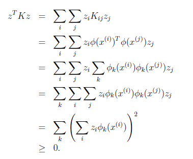
which showed that $K$ is positive semi-definite.

Theorem: Mercer

Let $K: \mathbb{R}^n \times \mathbb{R}^n \mapsto \mathbb{R}$ be given. Then for $K$ to be a valid Mercer Kernel, it is necessary and sufficient that for any ${x^{(1)}, x^{(2)},…,x^{(m)}}$, the corresponding kernel matrix $K$ is symmetric positive semi-definite

Take Away Message

The Kernel trick is actually more fundamental than the SVM. In general, if you have any learning algorithm that uses $\lang x^{(i)}, x^{(j)} \rang$, you can swap it with $K(x,z)$ and apply the learning in a much higher dimensional space.

Regularization and the Non-Separable Case

However, the algorithms above still have the assumption that data is separable in some higher dimensions. What if due to some noise in the data, they are (intrinsically) not separable (or you want to prevent it from overfitting)?

e.g. data with some noise:

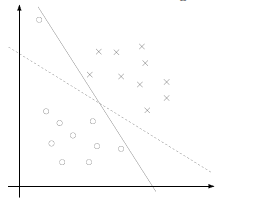
where having just one outlier, we need to move the boundary dramatically.

To make the algorithm work for non-linearly separable datasets as well as be less sensitive to outliers, we reformulate our optimization task to use the $\ell_1$ regularization:

\[\begin{align*} \min_{w,b,\xi} &\quad \frac{1}{2}||w||^2 + C \sum_{i=1}^m \xi_i\\ \text{s.t.} &\quad y^{(i)}(w^T x^{(i)} + b) \ge 1 - \xi_i,\quad i=1,...,m \\ &\quad \xi_i \ge 0 , \quad i=1,...,m \end{align*}\]

where:

on the bottom, we relaxed the constraint to be $1 - \xi_i$, which is easier to satisfy. In fact, as long as $1 - \xi_i > 0$, we have a correct guess
on the top, we are minimizing $\frac{1}{2}\vert \vert w\vert \vert ^2 + C \sum_{i=1}^m \xi_i$, with the additional term added such that the $1-\xi_i$ will not have $\xi_i$ being too large
The parameter $C$ controls the relative weighting between the twin goals of making the $\vert \vert w\vert \vert ^2$ small (which we saw earlier makes the margin large) and of ensuring that most examples have functional margin at least $1$.

Graphically, you can think of the error term $\xi$ being the red cross in the image:

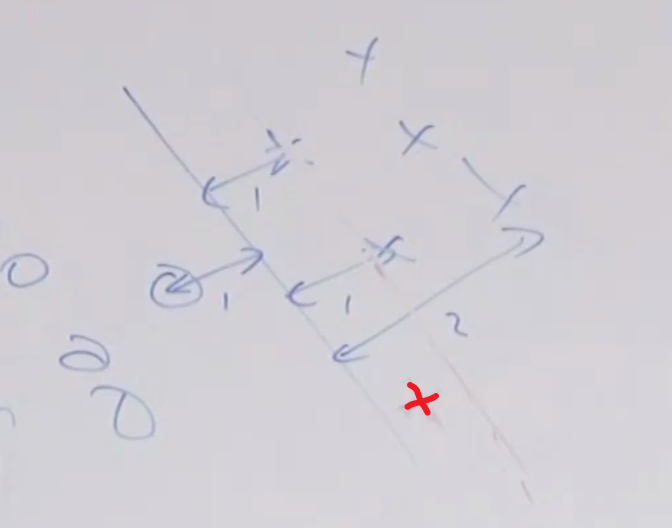
where:

if you required strictly $\ge 1$, then the boundary cannot be the one in the image since the closest samples must have functional margin of $1$ (where as the red cross is clearly less than 1)
if you relaxed the condition and asked for $\ge 0.5$ say, then the red cross (suppose if having a functional margin of 0.51) would be allowed in this given boundary.

Lastly, we use the same approach in Lagrange Duality and simplify $\ell_1$ optimization problem to:

\[\begin{align*} \max_{\alpha} &\quad \sum_{i=1}^m \alpha_i - \frac{1}{2} \sum_{i,j=1}^m \alpha_i \alpha_jy^{(i)}y^{(j)} \lang x^{(i)},x^{(j)} \rang\\ \text{s.t.} &\quad 0 \le \alpha_i \le C,\, i=1,...,m\\ &\quad \sum_{i=1}^m \alpha_i y^{(i)} = 0 \end{align*}\]

where:

after computing the optimal $\alpha$, you can then compute $w$ using Equation 102. However the optimal $b$ would be changed.
the parameter $C$ is something you need to choose. This will be discussed in the future sections.

The SMO Algorithm

Check notes

Learning Theory

This section talks about many techniques that you can use in real life when dealing with ML.

Bias and Variance

Recall that in section Overfitting and Underfitting, we discussed things that could go wrong when we chose a “wrong” hypothesis:

Consider the data being actually distributed in $x \mapsto O(x^2)$, such that we have:

Underfitting/High Bias	Actual	Overfitting/High Variance

where:

first figure is underfitted as we only imagined $y = \theta_0 + \theta_1 x$. We also call it high bias.
third figure is overfitting as we imaged $y=\theta_0 + \theta_1 x + \theta_2 x^2 + … + \theta_5 x^5$. We also call it high variance
both first and third figure will have a very large generalization error. (informally, think of it as expected error on examples not necessarily in the training set.)

Bias (informal)

high bias: then even if we were fitting a linear model to a very large amount of training data, the linear model would still fail to accurately capture the structure in the data.

Informally, we define the bias of a model to be the expected generalization error even if we were to fit it to a very (say, infinitely) large training set.

Variance (informal)

fitting patterns in the data that happened to be present in our small, finite training set, but that do not reflect the wider pattern of the relationship between $x$ and $y$.

Most of the time, we need to consider tradeoffs:

If our model is too “simple” and has very few parameters, then it may have large bias (but small variance)
if it is too “complex” and has very many parameters, then it may suffer from large variance (but have smaller bias).

In a slightly more formal view, consider the case where you need to fit 2 parameters, $\theta_1, \theta_2$, from $4$ different learning models. Suppose you have some distribution $\mathcal{D}$ where you draw samples $(x,y)$ from:

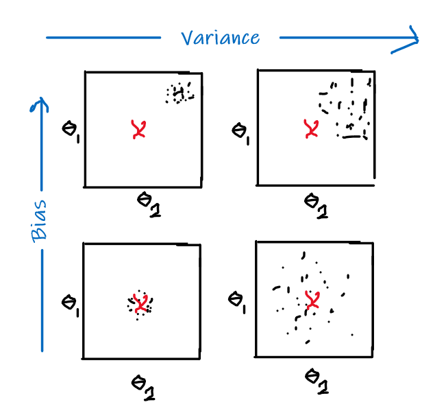
where:

the red cross is the “true value” of $\theta_1^, \theta^_2$
each black dot represent, for each $m$ times you sampled, which obtained a training set $S$ of size $m$, you compute the ERM of $\theta_1, \theta_2$ for each model

Therefore, you see that:

a low bias corresponds to the case where $\theta_1, \theta_2$ are close to the “true parameter” across different samples of training set $\mathcal{D}$
- so a zero bias would be mean $E[\hat{\theta}] = \theta^*$ for some $m$.
a low variance corresponds to the case where $\theta_1, \theta_2$ are close to each other across different samples of training set $\mathcal{D}$

This means that:

if you were able to collect an infinite number of samples, $m \to \infty$, then the data points will be more concentrated. This means that $\mathrm{Var}[\theta] \to 0$. This is also called statistical efficiency (the rate of which $\mathrm{Var}[\theta] \to 0$).
- this would be related to variance
if $m \to \infty$ and $\hat{\theta} \to \theta^*$, then this is called statistical consistency.
- this would be related to bias. If bias is too high, then it might not be.

Preliminaries

This section aims to answer questions such as: Why should doing well on the training set tell us anything about generalization error? Specifically, can we relate error on the training set to generalization error?

Lemma Union Bound

Let $A_1, … A_k$ be $k$ different events (that may not be independent). Then:
\[P(A_1 \cup \dots \cup A_k) \le P(A_1) + \dots +P(A_k)\]

Lemma Hoeffding Inequality

Let $Z_1, …,Z_m$ be $m$ independent and identically distributed (IID) random variables (i.e. if it is binary classification, then $Z_i = {0,1}$) drawn from a Bernoulli $(\phi)$ distribution. I.e. $P(Z_i =1) = \phi$, then $P(Z_i=0)=1-\phi$.

Let $\hat{\phi}$ be the mean of those variables, such that:
\[P(|\phi - \hat{\phi}| > \gamma) \le 2 \exp{ (-2 \gamma^2 m )}\]
which basically says that if take the mean $\hat{\phi}$ to be the estimate for $\phi$, then the probability of us being far away from the true value is small if $m$ is large.

for instance, if you have a biased coin with a chance of $\phi$ landing on heads, then each toss independently has a $P(Z_i=1)$ probability of being head. If you toss it $m$ times and compute the mean, i.e. fraction of times that it landed up in head, then that will be a good estimate of the true $\phi$ if $m$ is large enough.

To start off, we restrict our attention to binary classification in which the labels are $y\in {0,1}$. Though everything here can be generalized to others, including regression and multi-class classification.

Consider a training set $S = { (x^{(i)},y^{(i)}) }_{i=1}^m$, where the training samples are drawn IID from the same distribution $\mathcal{D}$. Then for a hypothesis $h$, we can define the training error (also called the empirical risk or empirical error) to be:

\[\hat{\varepsilon}_S(h) = \hat{\varepsilon}(h) = \frac{1}{m} \sum_{i=1}^m 1\{h(x^{(i)}) \neq y^{(i)}\}\]

which is basically fraction of times the hypothesis misclassified.

note that we used $\hat{\varepsilon}_S(h)$ because this also depends on the dataset we are using for training

Then, we define the generalization error to be:

\[\varepsilon(h) = P_{(x,y) \sim \mathcal{D}} (h(x) \neq y)\]

which means that the probability of $h$ misclassifying if we draw a new sample $(x,y)$ from the same distribution $\mathcal{D}$.

the assumption that both the training data and the test data are from the same distribution $\mathcal{D}$ is called the PAC (probably approximately correct) assumptions.

Empirical Risk Minimization (ERM)

Consider the setting of linear classification such that our hypothesis is $h_\theta(x) = 1{ \theta^T x \ge 0 }$. Then one approach for fitting the parameter $\theta$ is to minimize the training error:
\[\hat{\theta} = \arg \min_{\theta} \hat{\varepsilon}(h_\theta)\]

To be more abstract, we can consider any hypothesis by defining a hypothesis class $\mathcal{H}$ to be the set of all classifiers/hypothesis considered by it. A hypothesis class of linear classifiers would be:
\[\mathcal{H} = \{ h_\theta : h_\theta(x) = 1\{ \theta^T x \ge 0 \}, \theta \in \mathbb{R}^{n+1} \}\]
Therefore, empirical risk minimization would be though of minimizing over the class of functions in $\mathcal{H}$.
\[\hat{h} = \arg \min_{h \in \mathcal{H}} \hat{\varepsilon} (h)\]

Last but not least, sometimes it is useful to think of generalization error as components:

where each point on the graph represents a hypothesis.

Given some hypothesis class $\mathcal{H}$, and some data set $\mathcal{D}$, consider some best possible hypothesis $g$ (e.g. having the smallest generalization error, which might not be $0$). Then, we define the following:

$\varepsilon(g)$ = Bayes Error/ Irreducible Error
$\varepsilon(h^*) - \varepsilon(g)$ = Approximation Error
$\varepsilon(\hat{h}) - \varepsilon(h^*)$ = Estimation Error
therefore $\varepsilon(\hat{h}) = \text{Estimation Error} + \text{Approximation Error} + \text{Irreducible Error}$

Finally, this can be further broken down to:

\[\begin{align*} \varepsilon(\hat{h}) &= \text{Estimation Error} + \text{Approximation Error} + \text{Irreducible Error} \\ &= \text{Estimation Variance} + \text{Estimation Bias} + \text{Approximation Error} + \text{Irreducible Error} \end{align*}\]

where:

Estimation Variance is often called variance
Estimation Bias + Approximation Error is often called bias

Fighting Variance

Some techniques to reduce variance would be:

increase $m$
add regularization to the model
- the net effect can be thought of as decreasing the size of your hypothesis class

Fighting Bias

Some techniques to reduce bias would be:

make the hypothesis class $\mathcal{H}$ bigger
- note that this might increase variance

The problem is we kind of need to know the “true value” of parameter $\theta$ in advance.

The case of finite $\mathcal{H}$

Consider a finite hypothesis class $\mathcal{H} = { h_1, …, h_k }$ consisting of $k$ hypothesis, i.e. $\mathcal{H}$ is a a set of $k$ mappings from $\mathcal{X}$ to ${0,1}$. The empirical risk minimization selected a hypothesis $\hat{h}$.

We would like to give guarantees on the generalization error of $\hat{h}$. Our strategy for doing so will be in two parts:

First, we will show that $\hat{\varepsilon}(h)$ is a reliable estimate of $\varepsilon(h)$ for all $h$.
Second, we will show that this implies a connection between generalization error of the ERM $\varepsilon(\hat{h})$ and that of the best possible hypothesis $\varepsilon(h^*)$.

Take one fixed $h_i \in \mathcal{H}$. Consider a Bernoulli random variable $Z$, such that we sample $(x,y) \sim \mathcal{D}$, and $Z=1{ h_i(x) \neq y }$. Similarly, we define $Z_j = 1{ h_i(x^{(j)}) \neq y^{(j)} }$. Since our samples are drawn IID from $\mathcal{D}$, then random variable $Z$ and $Z_i$ has the same distribution.

where basically:

we sampled some randomly sampled dataset $\mathcal{D}$ from the distribution, and for all hypothesis $h \in \mathcal{H}$, we calculated the generalization error $\varepsilon$ and the training error based on the sampled dataset $\hat{\varepsilon}_S$
for any hypothesis $h_i$, we can say that, if we do the sampling of dataset many times and for each time compute the training error, we will get:
\[E[\hat{\varepsilon}(h_i)] = \varepsilon(h_i)\]
i.e. the average of those training error lines will converge to the generalization error.

What is the misclassification probability on a randomly drawn example? (if we have only sampled a finite dataset $\mathcal{D}$)

This is exactly the expected value of $Z$.

Moreover, since the training error can be written as:

\[\hat{\varepsilon}(h_i) = \frac{1}{m} \sum_{j=1}^m Z_j\]

now, notice that:

$\hat{\varepsilon}(h_i)$ is exactly the mean of $m$ random variables $Z_j$ that are drawn IID from a Bernoulli Distribution with mean $\varepsilon(h_i)$.
now we can use Hoeffding Inequality, since we have the mean of some random variables from some distribution.

Therefore, applying the Hoeffding Inequality, we obtain:

\[P(|\varepsilon(h_i) - \hat{\varepsilon}(h_i)| > \gamma) \le 2 \exp( -2\gamma^2 m )\]

which shows that

for our particular $h_i$, training error will be close to generalization error with high probability, assuming $m$ is large.
basically, the green line above will be closer to the blue line if $m$ is large.

This proved that for one particular $h_i$, training error is close to generalization error. We want to prove that this will be true for simultaneously $\forall h \in H$.

i.e. we want to have the entire green line converge uniformly to the blue line in the figure above.

To do so, let $A_i$ denote the event that $\vert \varepsilon(h_i) - \hat{\varepsilon}(h_i) \vert > \gamma$. Then for any particular $A_i$, we know that $P(A_i) \le 2 \exp(-2\gamma^2 m)$. Using the union bound, we get:

\[\begin{align*} P(\exists h \in \mathcal{H}, |\varepsilon(h_i) - \hat{\varepsilon}(h_i) | > \gamma) &= P(A_1 \cup \dots \cup A_k) \\ &\le \sum_{i=1}^k P(A_i) \\ &\le \sum_{i=1}^k 2 \exp(-2 \gamma^2 m)\\ &= 2k \exp(-2\gamma^2 m) \end{align*}\]

which is pretty intuitive because we have $k$ hypothesis.

Therefore, we get:

\[P(\exists h \in \mathcal{H}, |\varepsilon(h_i) - \hat{\varepsilon}(h_i) | \le \gamma) \ge 1- 2k \exp(-2\gamma^2 m)\]

so that with at least $1-2k \exp(-2\gamma^2 m)$ probability we will get $\varepsilon(h)$ within $\gamma$ to $\hat{\varepsilon}(h)$ for all $h \in \mathcal{H}$. This is called a uniform convergence result, because this is a bound that holds simultaneously for all (as opposed to just one) $h \in H$.

So the important parameters here would be:

$\delta \equiv 2k \exp(-2\gamma^2 m)$ probability of error
$\gamma$ margin of error
$m$ sample size

For instance

we can ask the following question: Given $\gamma$ and some $\delta > 0$, how large must $m$ be before we can guarantee that with probability at least $1 − \delta$, training error will be within $\gamma$ of generalization error?

We can solve this by setting $\delta = 2k \exp(-2\gamma^2 m)$ and solve for $m$, which gives:

\[m \ge \frac{1}{2\gamma^2} \log{\frac{2k}{\delta}}\]

such that:

with probability at least $1-\delta$, we have $\vert \varepsilon(h_i) - \hat{\varepsilon}(h_i) \vert > \gamma$ for $\forall h \in \mathcal{H}$.
This bound tells us how many training examples we need in order make a guarantee, which is also called the sample complexity.

Previously we have shown a connection between training error $\hat{\varepsilon}(h)$ and the generalization error $\varepsilon(h)$.

Next, we show the connection between the generalization error from the ERM $\varepsilon(\hat{h})$ and that of the best in class $\varepsilon(h^*)$.

\[\begin{align*} \varepsilon(\hat{h}) &\le \hat{\varepsilon}(\hat{h}) + \gamma \\ &\le \hat{\varepsilon}(h^*) + \gamma \\ &\le \varepsilon(h^*) + 2\gamma \end{align*}\]

where:

The first line used the fact that $\vert \varepsilon(\hat{h}) - \hat{\varepsilon}(\hat{h})\vert \le \gamma$ (by our uniform convergence assumption).
The second line used the fact that $\hat{h}$ minimizes training error
The third line used the uniform convergence again, since this $\gamma$ is "shared" across all hypothesis.

We can solve for $\gamma$ using the equation 141 above, and this gives the thorem:

Bound on Generalization Error:

Let $\vert \mathcal{H}\vert = k$, and let some $m, \delta$ be fixed. Then with probability at least $1-\delta$, the following is true:
\[\varepsilon(\hat{h}) \le \varepsilon(h^*) + 2 \sqrt{\frac{1}{2m}\log \frac{2k}{\delta}}\]
where:

we basically solved for the $\gamma$ in the equation mentioned previously.

the $h^*$ would be the hypothesis with lowest point on the blue line

The case of infinite $\mathcal{H}$

Basically the idea is to “assign size” to hypothesis class with infinite numbers of hypothesis. This is done by the concept of VC-dimension.

Key results shown first, which is similar to equation 143:

\[\varepsilon(\hat{h}) \le \varepsilon(h^*) + O\left(\sqrt{\frac{d}{m}\log \frac{m}{d}+ \frac{1}{m}\log \frac{1}{\delta}}\right)\]

where:

$d=\mathrm{VC}(\mathcal{H})$ is the VC-dimension of some hypothesis class $\mathcal{H}$

Regularization and Model Selection

Regularization is a very useful technique to prevent use from overfitting.

For Example:

Recall the simple least square error that we are trying to minimize:

\[\min_\theta \frac{1}{2}\sum_{i=1}^m || y^{(i)} - \theta^T x^{(i)} ||^2 + \frac{\lambda}{2} ||\theta||^2\]

where we have added the term $(\lambda/2 )\vert \vert \theta\vert \vert ^2$ to prevent $\theta$ being to large. If $\theta$ is unconstraint, then learning algorithms might end up with (assuming a hypothesis of fifth order polynomial)

Overfitting with $\lambda = 0$	$\lambda = 1$	Underfitting with $\lambda = 100$

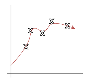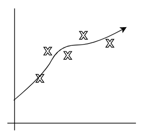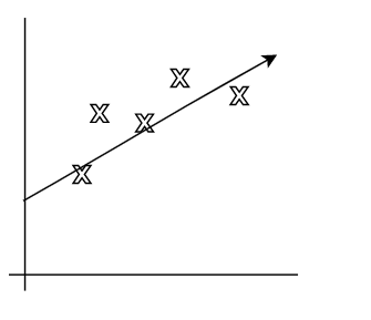the idea is that there is usually some optimial $\lambda$ that can result in some really good fits.

Similarly, for logistic regression, we can have:

\[\arg\max_\theta \sum_{i=1}^m \log{\left(p(y^{(i)}|\theta^Tx^{(i)}) \right)} - \frac{\lambda}{2} ||\theta||^2\]

in a similar manner.

Note

In fact, the term $\vert \vert w\vert \vert ^2$ in SVM:

also prevents SVM to be overfitting. It has a similar effect as the ones mentioned above.

Proof (Informal)

The proof for the regularization idea is as follows.

Consider a training set $S={(x^{(i)}, y^{(i)})}_{i=1}^m$, and that our model relies on some parameter $\theta$. Then consider the probability:

\[\begin{align*} \arg\max_{\theta} p(\theta | S) &=\arg\max_{\theta} \frac{p(S|\theta)p(\theta)}{p(S)}\\ &=\arg\max_{\theta} p(S|\theta)p(\theta)\\ \end{align*}\]

for logistic regression (or other generalized linera model):

\[\begin{align*} \arg\max_{\theta} p(\theta | S) &=\arg\max_{\theta} p(S|\theta)p(\theta)\\ &= \arg\max_{\theta}\left( \prod_{i=1}^m p(y^{(i)}|x^{(i)}, \theta) \right)p(\theta) \end{align*}\]

and assuming probability of $\theta$ being distributed normally:

\[p(\theta): \theta \sim \mathcal{N}(0, \tau^2 I)\]

then computing the quantity $\arg\max_{\theta} p(\theta \vert S)$ will yield the term $\vert \vert \theta\vert \vert ^2$ for regularization.

Frequentist School:

the canonical idea is to find the most likely $\theta$ given the dataset $S$. Therefore, it talks about maximum likelyhood estimation (MLE)
\[\arg\max_\theta p(S|\theta)\]

Bayesian School:

the idea here is that the parameters $\theta$ are distributed by a normal distribution $\theta \sim \mathcal{N}(0, \tau^2 I)$ a priori to the dataset. Hence it computes the probability of having a $\theta$ given the dataset $S$ by the maximum a posterior (MAP)
\[\arg\max_{\theta}p(\theta|S)\]

in fact, the regularization idea would be also derived from the Bayesian prior

Graphically, the difference between biases and variance is shown below:

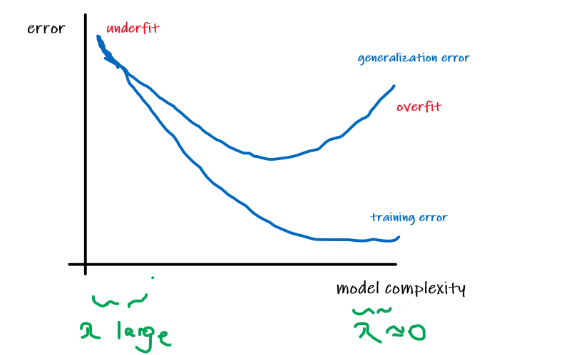
where:

obviously our aim is to get the $\lambda$ regularization such that our model ended up in the middle, which has the smallest generalization error.

Cross Validation

Let’s suppose we are, as usual, given a training set $S$. Given what we know about empirical risk minimization, here’s what might initially seem like a algorithm:

Train each model $M_i$ on $S$, to get some hypothesis $h_i$ form each model
Pick the hypothesis with smallest training error

This naïve idea would not work. Consider the case of having models $M_i$ of polynomial with degree $i$. Then hypothesis from model with a higher order of polynomial will always fits better on the training set $S$.

Hold-Out Cross Validation/Simple Cross Validation

One remedy from the above approach it to split the data into $S_{\mathrm{train}}, S_{\mathrm{cv}}, S_{\mathrm{test}}$, such that:

Randomly split the data into $S_{\mathrm{train}}$, e.g. 70% of the data, and $S_{\mathrm{train}}$ (optionally $S_{\mathrm{test}}$) the remaining

sometimes, the cross validation set is also called the “dev set” $S_{\mathrm{dev}}$.

Train each model $M_i$ on $S_{\mathrm{train}}$ only, to get some hypothesis $h_i$

Select and output the hypothesis with smallest error on $S_{\mathrm{cv}}$, such that $\hat{\varepsilon}{S{\mathrm{cv}}}(h_i)$ is smallest.

(Optionally) If you need to publish your result/use it somewhere, you can then compare the hypothesis by putting them through $S_{\mathrm{test}}$

the take-away message is that your $S_{\mathrm{test}}$ set should not be seen any where in the training/decision of your models. Otherwise such evaluation metrics is meaningless as you are fitting your data towards it.

Some of the commonly used splitting size would be $S_{\mathrm{train}}=60\%, S_{\mathrm{cv}}=20\%, S_{\mathrm{test}}=20\%$. However, if your data set is really large, then having lots of test samples might not make sense unless you care about very small improvements, e.g. $0.01\%$ difference. Therefore, often it might become $S_{\mathrm{cv}}=5\%, S_{\mathrm{test}}=5\%$ if your data size is very big.

However, one disadvantage of this is that some of the data is “wasted” as they are used for evaluation but not training. When your dataset is small, this might be a problem.

Now to make the illustration easier, consider the case where we have already prepared our $S_{\mathrm{test}}$. Then one approach to “save” some data when you are at a small dataset is to have:

$k$-fold Cross Validation

Randomly split $S$ into $k$ disjoint subsets of equal size. Let’s call those subsets $S_{1},\dots, S_k$

For each model $M_i$, do the following:

so that basically you have used all your data at least once for training.

Pick the model $M_i$ which outputted the hypothesis with the lowest estimated averaged generalization error.

(Optionally) Once you have decided which model to use, i.e. model with polynomial of degree 3, then retrain the model on the entire training set for later production use.

In practice, $k=10$ is most commonly used. However, the problem with this is that it is computationally more expensive, since each model is trained $k$ times. Therefore, this is a good idea only if your data size is small.

Feature Selection

Another useful technique to prevent from overfitting is to consider a subset of $n$ features that are relevant to the learning task.

Consider the case where you want to find a subset of $n$ given features for your training. Given $n$ features, there are $2^n$ possible feature subsets (since each of the $n$ features can either be included or excluded from the subset), and thus feature selection can be posed as a model selection problem over $2^n$ possible models, which is a lot.

For large $n$, usually some other heuristic search procedure is used to save some computational power.

Forward Search Procedure

Start with the set of features to use $\mathcal{F} = \empty$.

Repeat, until no improvements on generalization error (or other stopping condition):

For feature $F_i,i=1,\dots, n$, and that $F_i \notin \mathcal{F}$, try $\mathcal{F}_i = \mathcal{F}\cup {F_i}$. Then we use the cross validation technique to check if there is any improvements on generalization error.

Select $\mathcal{F}$ to be the best feature subset (e.g. with smallest generalization error) for the next iteration

Output the found $\mathcal{F}$

In other words, this is basically a greedy algorithm that takes the best result at current iteration and use it for the future. However, this is still computationally expensive, but useful.

Decision Tree and Ensembles

Consider the prediction for which month of the year we can go to ski. Depending on the latitude (“height”) you are living at, we know that:

where:

at high latitudes (north), winter comes earlier; at low latitudes (south). winter comes later

Since the problem now becomes distinguishing the regions, we could:

use SVM with casting those features into higher dimensional space
more naturally, the decision tree model

Decision Tree Model

The model is our first example of a intrinsically non-linear model.

In general, it is a model of a greedy, top-down, recursive approach.

For example

To solve the problem above, we might end up with asking the questions:

graph TD
    Lat_larger_30 --> |Yes|Month_less_3
    Lat_larger_30 --> |No|Month_larger_3
    Month_less_3 --> |Yes| ...
    Month_less_3 --> |No| ....

where:

this is a greedy algorithm because in each step, it decides the “currently best split”
it is recursive since for each new question becomes the root

In the end, we will basically obtain:

Therefore, the idea is for a region of data $R_p$, we need some split $s_p$ such that:

\[s_p(j,t) = \begin{cases} \{ x|x_i < t,\,x \in R_p \} & \equiv R_1\\ \{ x|x_i \ge t,\,x \in R_p \} & \equiv R_2 \end{cases}\]

where:

$j$ is the j-th feature you are splitting/looking at
$t$ is the threshold value for splitting
this splitting splits the region $R_p$ into two regions $R_1, R_2$

To decide which split to take on, we need to define a loss for each split, and then pick the smallest lost. First we need to define a few things to make this formal:

$L(R)$ is the loss on a region $R$
$C$ is the number of classes in our data
$\hat{p}_c$ is the proportion of data in $R$ that are in the class $c$

In our tree model, we would have for each node:

\[\max_{j,t}(L(R_p) - (L(R_1) + L(R_2)))\]

where:

$L(R_p)$ is basically defined by the precious parent node, so it is a constant here
$L(R_1), L(R_2)$ are the loss of the children, so they needs to be optimized with $j,t$
so basically we want to minimize the loss of children

For Example: Simple Misclassification Loss

Then a one naive way of minimizing misclassification is to define:

\[L_{\mathrm{misclass}} = \text{number of misclassified data}\]

Then the following splits would be evenly good

where:

the root note basically predicts everything to be positive (since there are more positives), so 100 samples are missclassified
all the children nodes in this case predicts positive, since there are more positives in the node.

So you see that even though the number of misclassified samples is the same for both models, many would argue that the right one is better since it isolated out more positive samples.

So if you draw the shape:

Therefore, we need one possibility would be something like cross-entropy loss:

\[L_\mathrm{cross} = - \sum_c \hat{p}_c \log_2 \hat{p}_c\]

This has the advantage of a concave curve for loss.

If the split is even, i.e. 500 data to the left and 500 data to the right, then we will see:

where the shape for $L$ gives:

the change in loss $\max_{j,t}(L(R_p) - (L(R_1) + L(R_2)))$ would be the gap drawn in the figure.

Another would be the Gini loss:

\[\sum_c \hat{p}_c (1-\hat{p}_c)\]

and this has a similar shape to that of the cross-entropy loss above.

Note

decision trees like this face a problem of overfitting if you let the tree grow freely, such that it will have eventually each node itself being a region. This demonstrates the high variance nature of decision tree. To solve this issue, check out the section Regularization of Decision Trees

Another problem is that it has no additive structure. If you have a data generated where the separation is simply a slant line, then decision tree would need to do lots of work.

Regression Tree

The above basically uses decision tree for classification. We could also do the problem of regression using this model.

Consider the same case for skiing, where we have some continues values such as:

For prediction, you would basically predict the average value inside some region $R_m$:

\[\hat{y}_m = \frac{\sum_{i \in R_m} y_i}{|R_m|}\]

In this case, your loss would be defined as:

\[L_{\mathrm{squared}} = \frac{\sum_{i \in R_m}(y_i - \hat{y}_m)^2}{|R_m|}\]

which basically would deal with the purity of data inside some region $R_m$.

Regularization of Decision Trees

Some common approaches in this case would be:

min leaf size (how many nodes in each leaf/region)
max depth of tree
max number of nodes
minimum decrease in loss (this might cause an issue of early-stopping, if you have some higher order correspondence)
pruning (grow the tree first, then prune it using misclassification of validation set data)

Runtime

What actually happens at run time would be the following.

First, consider the case of having:

$n$ examples/data samples
$f$ features for each sample
$d$ depth of our result tree

Then we would have gone through:

	Train Time	Test Time
Computation Time	$O(nfd)$	$O(d)$ since we are going through the tree

where:

commonly $d < log_2n$
train time is $O(nfd)$ because the cost of each sample at each node is $O(f)$, since you basically just need try $f$ questions, and each sample is part of $O(d)$ nodes (do it $O(d)$ times), i.e. your data matrix would be $nf$.
Therefore, since depth is usually $log_2 n$, so it is generally a fast algorithm

Summary

For the decision tree model we covered just now:

Advantage	Disadvantage
Easy to explain	High Variance
Result/model interpretable	Bad at data being additive
Fast	Low predictive accuracy (due to the two above)
Categorical Variables also work

where:

Low predictive accuracy hurts a lot

Therefore, usually what we do is to have an ensemble of decision trees.

Ensemble

Consider the case of having $n$ random variables $x_i$ being IID. And suppose that the distribution has $\mathrm{Var}(x_i) = \sigma^2$.

Then given the assumption results in:

\[\mathrm{Var}(\bar{x}) = \mathrm{Var}\left(\frac{1}{n}\sum_i x_i\right) = \frac{\sigma^2}{n}\]

Sometimes, your random variable will be correlated. Suppose they are correlated by $\rho$. Then we have $x_i$ being distributed ID, and that:

\[\mathrm{Var}(\bar{x}) =\rho\sigma^2 + \frac{1-\rho}{n}\sigma^2\]

wheree:

notice that if they are completely correlated, $\rho=1$, then the average of the variance is just the variance of one variable
if they are completely independent, $\rho=0$, then you restore equation 157.

Idea

Now, the idea is to consider each random variable being our model itself, sampled from some distribution. Our aim is to get a final aggregated model that who comes from a distribution of a lower variance. Therefore, effectively we want to "average/ensemble" different models to improve the performance, i.e. achieve lower variance.

Now, some ways to achieve ensemble mentioned above, some methods include:

having different learning algorithms (e.g. decision tree, regression, SVM, etc.)
having different training data set
[more commonly used] bagging, e.g. random forest
[more commonly used] boosting, e.g. xgboost

Bagging - Bootstrap Aggregation

Bagging stands for bootstrap aggregation.

Basically, the idea is to have

assume your entire train dataset to be the true population $P$
each training set $Z_i$ is sampled without replacement from $P$
each tree model $G_i$ is then trained on $Z_i$
the final result is the average result of all models $G_i$

To be more specific, suppose you have $M$ models trained. Now given a new input $x’$, you basically do:

\[G_{\mathrm{final}}(x') = \frac{\sum_{i=1}^m G_i(x')}{M}\]

The net effect is that the variance of your model decreases since:

$\frac{1-\rho}{n}\sigma^2$ in equation 158 will be decreased since $M=n$ basically increases as the number of trained model increases
$\rho$ in equation 158 will also be decreased since bootstrapping make them less corelated

However, the drawback is that your bias would increase (slightly) since:

each model is trained on less data/random subsampling

Bagging + Decision Tree

Recall that decision trees have high variance but low bias. Therefore, this works nicely with Bagging.

Random Forest

Basically it is the Bagging approach + more decorrelation of models, to further drive $\rho$ down.

This is achieved by considering only a fraction of features at each split, which would result in lower correlation between models.

think of the case where there is a strong feature that works nicely for classification. Then most of your trees will have that being the first split, hence somewhat correlated. However, this can be avoided if you force only a fraction of features being considered.

Boosting

This is more like the opposite, it is decreasing the bias but increasing the variance. The key difference is that this approach is about addition.

The basic idea is as follows (this is actually ADABoost):

train a tree $G_i$ by forcing a depth of $1$ (so by only allowing to ask one question, we want to minimize variance)
compute the error of this model $\mathrm{err}_i$ and assign this model a weight $\alpha_i \propto \log(\frac{1-\mathrm{err_i}}{\mathrm{err_i}})$
reweight the misclassified samples in this model
repeat step from step 1

Now, when you get $M$ trees, your final result $G$ is basically, for a new data $x’$:

\[G(x') = \sum_{i=1}^M \alpha_i G_i(x')\]

For more details, read the extra-notes.

Introduction to Neural Network

Heuristics:

we will start with logistic regression (revision), and then go to neural network from it
then we talk a little bit about deep learning (a set of techniques/algorithms)
- different from other algorithm, DL are computationally expensive, and the data used is usually large

For instance, consider the task of finding cats in images. If there is a cat in the image, output 1, otherwise 0.

suppose images are of size $64\times 64$. Then you basically have a $64 \times 64 \times 3$ numbers.

Then, what we can do is:

convert each picture to a vector, of size $(64\times 64 \times 3, 1)$
feed the vector into a logistic regression algorithm, which basically learns $\theta$ for the sigmoid function we discussed before: $1/(1+e^{-\theta^T x}) \equiv \sigma(\theta^Tx) = \sigma(w^Tx + b)$
finally, we just output $\hat{y} = \sigma(\theta^T x) = \sigma(w^Tx + b)$. Usually $w$ is called weights and $b$ is called bias here.

Therefore, the learning algorithm basically does:

initiate some $w, b$
find the optimal $w, b$. This means that we need to define a loss function.
output $w,b$

Recall that for logistic regression, we had the logistic loss, and we want to minimize:

\[\mathcal{L} = - [y\log(\hat{y})+(1-y)\log(1-\hat{y})]\]

which comes from maximizing the log likelihood.

Then, we can basically find the optimal by doing gradient descent:

at every batch of data, compute $w:=w - \alpha \frac{\partial \mathcal{L}}{\partial w}$, $b:=b - \alpha \frac{\partial \mathcal{L}}{\partial b}$

Now, we show you how it can evolve into a neuron network.

Terminologies and Introduction

Some common terms to know would be:

Neuron = Linear + Activation

In the case of logistic regression, the part $w^T x + b$ is the linear part, and the $\sigma(w^Tx + b)$ is the activation
Model = Architecture + Parameter

In the case of logistic regression, we have an architecture of 1 neuron, and the parameter $w, b$

Example

Consider now the goal of finding a cat/lion/iguana in the image.

Then, since we have three “tasks” to find, we can use three neurons:

where:

basically the input is linked/goes through all neurons $a_i^{[1]}$
the subscript $[1]$ means we are at the first layer. Later on we will show a multilayered one.
therefore, basically the parameters becomes $\left(w_1^{[1]}, b_1^{[1]}\right), \left(w_2^{[1]}, b_2^{[1]}\right), \left(w_3^{[1]}, b_3^{[1]}\right)$
since we have this architecture, then the label should look like $[1, 0, 0]^T$ (if it is a cat). For a lion $[0,1,0]^T$. The good part of this is that then the job of each neuron is clear and simple.

Note that in this case, this will be robust since if you have a picture containing both a cat and a lion, i.e. $[1,1,0]^T$, then it will still work. In fact, this is due to the neurons as being decoupled, and also our images are generated independently.

Therefore, the loss technically becomes:

\[\mathcal{L}_{3\mathrm{neurons}} = -\sum_{k=1}^3 [y_k\log(\hat{y}_k)+(1-y_k)\log(1-\hat{y}_k)]\]

which sums up the three components, but additionally note that (taking $\mathcal{L}{3N} = \mathcal{L}{3\mathrm{neurons}}$):

$\partial \mathcal{L}_{3N}/{\partial w_i^{[1]}}$ has the same result as $\partial \mathcal{L}/{\partial w}$ since the variables $w_i^{[1]}$ are decoupled

However, one problem is that if the data is unbalanced, then some neurons might not be trained as much as others.

one way to deal with it is to use the SoftMax regression, which basically outputs the most likely instead of all three

For Example:

Consider the case where our goal is to find cat/lion/iguana in the image, but we are told that each image only contains one animal.

Then we can use the SoftMax regression, which basically gives the probability of the best possible classification (we talked about it before in multi-class classification):

where each neuron outputs:

$e^{z_i^{[1]}}/\sum_{k=1}^3 e^{z_k^{[1]}}$ and $z_i^{[1]} \equiv w_{i}^{[1]} x + b_{i}^{[1]}$ includes the parameters

Since now they are coupled, we need to define a different loss function to make the gradient descent easier:

\[\mathcal{L}_{CE} = \sum_{k=1}^3 y_k \log{\hat{y}_k}\]

where $\mathcal{L}_{CE}$ is the cross entropy loss.

Neural Networks

Now let’s consider the same task, to find a cat in an image, but with a more complicated neural network:

where the restriction is that:

for classification of $n$-classes, we should have the last layer consisting of $n$ neurons
for regression, the last layer should have only $1$ neuron
in each layer, neurons are disconnected
the second layer is also called the hidden layer, since it does not directly touch the input or the output

Notice that if the input vector has size $(n,1)$, then we will have $(3n+3) + (2\times 3 + 2) + (1\times 2 + 1)$ parameters. If we train this network, we will get typically the first layer recognizing edges in the image, second layer recognizng things like “ears”, “mustache” of the cat, and the last neuron figures out if there is a cat or not.

Another example would be to predict the house price given information such as size, zip code, etc.

One sensible idea to do it by hand would be:

note that some key differences here are:

inputs are no longer fully connected to the neurons in the first level

(as we go on, neural network will usually be able to figure which inputs are interesting by themselves. The idea is to first fully connect the network, and then allow weights.)
sometimes this is also called End-to-End learning/Black Box. This is because usually we will have no idea how/how to interpret the hidden layers in the middle will do.

Propagation Equation

Now let’s deal with the math of how this learning mentioned above work. Recall this setup:

First, we have:

$z^{[1]} = w^{[1]}x + b^{[1]}$ being the linear of first layer, and $a^{[1]} = \sigma(z^{[1]})$ being the activation
$z^{[2]} = w^{[2]}a^{[1]} + b^{[2]}$ being the linear of second layer, and $a^{[2]} = \sigma(z^{[2]})$ being the activation
$z^{[3]} = w^{[3]}a^{[2]} + b^{[3]}$ being the linear of third layer, and $a^{[3]} = \sigma(z^{[3]})$ being the activation

Note that a difference here is that we are using one equation for the entire layer. This means the shape of parameters is becoming:

$z^{[1]}\to (3,1);\quad w^{[1]}\to (3,n);\quad x\to (n,1)$ and the activation $a^{[1]}\to (3,1)$
$z^{[2]}\to (2,1);\quad w^{[2]}\to (2,3);\quad a^{[1]}\to (3,1)$ and the activation $a^{[2]}\to (2,1)$
$z^{[3]}\to (1,1);\quad w^{[3]}\to (1,2);\quad a^{[2]}\to (2,1)$ and the activation $a^{[3]}\to (1,1)$

Note

the architecture and the idea of having input propagated forward to get the output is also called forward propagation.

Now, if we have $m$ data points, then we consider the input of:

\[X = \begin{bmatrix} | & ... & |\\ x^{(1)} & ... & x^{(m)}\\ | & ... & | \end{bmatrix}\]

Then, the first linear part should have shape:

\[Z^{[1]} = w^{[1]}X + \tilde{b}^{[1]} = \begin{bmatrix} | & ... & |\\ z^{[1](1)} & ... & z^{[1](m)}\\ | & ... & | \end{bmatrix}\]

where:

$Z^{[1]} \to (3,m)$
$w^{[1]} \to (3,n)$ is the same as before
$\tilde{b}^{[1]} = \begin{bmatrix} | & … & |
b^{[1]} & … & b^{[1]}
| & … & | \end{bmatrix}$basically repeats the original stuff$m$ times to match the size

One advantage of using vectors is that we want to utilize our GPU to full capacity (parallel computation).

Optimization

Now we have the equations for each neuron, we need to consider the loss function and the cost function (cost usually refers to the error of the batch of $m$ examples, whereas loss refers to error of $1$ example).

Our task here is to optimize $w^{[i]}, b^{[i]}; i \in [1,3]$. Since the output is the last layer $\hat{y} = a^{[3]}$, we have the cost being:

\[\mathcal{J}(\hat{y}, y) = \frac{1}{m} \sum_{i=1}^m \mathcal{L}^{(i)}\]

and the loss can simply be the logistic loss:

\[\mathcal{L}^{(i)} = - [y^{(i)}\log(\hat{y}^{(i)})+(1-y^{(i)})\log(1-\hat{y}^{(i)})]\]

For a batch gradient descent, we know that we should get something like:

\[\forall l=1,...,3: \begin{cases} w^{[l]} := w^{[l]} - \alpha \frac{\partial \mathcal{J}}{\partial w^{[l]}} \\ b^{[l]} := b^{[l]} - \alpha \frac{\partial \mathcal{J}}{\partial b^{[l]}} \end{cases}\]

The question now is which layer should we start first? Since the idea of gradient descent is to move the parameters closer to the correct output, it makes more sense to start with the last layer first, since its effect on the output is the most obvious:

\[\frac{\partial \mathcal{J}}{\partial w^{[3]}} = \frac{\partial \mathcal{J}}{\partial a^{[3]}}\frac{\partial a^{[3]}}{\partial z^{[3]}}\frac{\partial z^{[3]}}{\partial w^{[3]}}\]

this computation of would make the later calculation easier, since:

\[\frac{\partial \mathcal{J}}{\partial w^{[2]}} = \frac{\partial \mathcal{J}}{\partial a^{[2]}}\frac{\partial a^{[2]}}{\partial z^{[2]}}\frac{\partial z^{[2]}}{\partial w^{[2]}} = \frac{\partial \mathcal{J}}{\partial z^{[3]}}\frac{\partial z^{[3]}}{\partial a^{[2]}}\frac{\partial a^{[2]}}{\partial z^{[2]}}\frac{\partial z^{[2]}}{\partial w^{[2]}}\]

notice that the quantity $\partial \mathcal{J}/{\partial z^{[3]}}$ was already computed in the previous equation 169, so it saved some work. Similarly, we do:

\[\frac{\partial \mathcal{J}}{\partial w^{[2]}} = \frac{\partial \mathcal{J}}{\partial z^{[2]}}\frac{\partial z^{[2]}}{\partial a^{[1]}}\frac{\partial a^{[1]}}{\partial z^{[1]}}\frac{\partial z^{[1]}}{\partial w^{[1]}}\]

Lastly, we just need to figure out the formula for $\partial \mathcal{J}/{\partial w^{[3]}}$.

Proof

First recall that when we take derivatives of a sigmoid function $\sigma$:

\[\sigma'(x) = \sigma(x)(1-\sigma(x))\]

in this case, since the activation layers are the sigmoid function, we have $a^{[i]} = \sigma(z^{[i]})$. For the last layer, notice that:

\[\hat{y} = a^{[3]} = \sigma(z^{[3]})=\sigma(w^{[3]}a^{[2]}+b^{[3]})\]

Therefore, some useful derivatives to compute beforehand would be:

\[\begin{align*} \frac{\partial \hat{y}}{\partial w^{[3]}} &=\frac{\partial \sigma(z^{[3]})}{\partial w^{[3]}} \\ &= \sigma'(z^{[3]}) \frac{\partial z^{[3]}}{\partial w^{[3]}} \\ &= \sigma(z^{[3]})(1-\sigma(z^{[3]})) \frac{\partial (w^{[3]}a^{[2]}+b^{[3]})}{\partial w^{[3]}}\\ &= a^{[3]}(1-a^{[3]})\frac{\partial (w^{[3]}a^{[2]}+b^{[3]})}{\partial w^{[3]}}\\ &= a^{[3]}(1-a^{[3]}) a^{[2]T} \end{align*}\]

Now, tarting with $\partial \mathcal{J}/{\partial w^{[3]}}$ by computing $\partial \mathcal{L}/{\partial w^{[3]}}$:

\[\begin{align*} \frac{\partial \mathcal{L}}{\partial w^{[3]}} &= - \left[y^{(i)}\frac{\partial }{\partial w^{[3]}}\log(\hat{y}^{(i)})+(1-y^{(i)})\frac{\partial }{\partial w^{[3]}}\log(1-\hat{y}^{(i)})\right] \\ &= - \left[ y^{(i)} \frac{1}{a^{[3]}}a^{[3]}(1-a^{[3]})a^{[2]T}+(1-y^{(i)})\frac{-1}{1-a^{[3]}}a^{[3]}(1-a^{[3]})a^{[2]T} \right] \\ &= -[y^{(i)}(1-a^{[3]})a^{[2]T}-(1-y^{(i)})a^{[3]}a^{[2]T}] \\ &= -[y^{(i)}a^{(2)T}-a^{[3]}a^{[2]T}]\\ &= - (y^{(i)}-a^{[3]})a^{[2]T} \end{align*}\]

where we assume $a^{[3]}$ is the activation/prediction for the $i$-th data sample.

Therefore, we easily obtain:

\[\frac{\partial \mathcal{J}}{\partial w^{[3]}} = \frac{-1}{m} \sum_{i=1}^m (y^{(i)}-a^{[3]})a^{(2)T}\]

This completes the computation for $\partial \mathcal{J}/{\partial w^{[3]}}$.

After we have $\partial \mathcal{L}/{\partial w^{[3]}}$, we need to consider how to obtain $\partial \mathcal{L}/{\partial w^{[2]}}$ using the result of $\partial \mathcal{L}/{\partial w^{[3]}}$, as we mentioned before. Notice that since $a^{[2]T}=\partial z^{[3]}/{\partial w^{[3]}}$:

\[\frac{\partial \mathcal{L}}{\partial w^{[3]}}=- (y^{(i)}-a^{[3]})a^{[2]T}=\frac{\partial \mathcal{L}}{\partial z^{[3]}}\frac{\partial z^{[3]}}{\partial w^{[3]}}\]

Therefore, knowing that $- (y^{(i)}-a^{[3]})={\partial \mathcal{L}}/{\partial z^{[3]}}$, we consider:

\[\begin{align*} \frac{\partial \mathcal{L}}{\partial w^{[2]}} &= \frac{\partial \mathcal{L}}{\partial z^{[3]}}\frac{\partial z^{[3]}}{\partial a^{[2]}}\frac{\partial a^{[2]}}{\partial z^{[2]}}\frac{\partial z^{[2]}}{\partial w^{[2]}}\\ &= (a^{[3]}-y)\cdot w^{[3]T} \cdot a^{[2]}(1-a^{[2]}) \cdot a^{[1]T} \\ &= w^{[3]T} * a^{[2]}(1-a^{[2]})\cdot (a^{[3]}-y)\cdot a^{[1]T} \end{align*}\]

where the last step needs some explanation:

the $*$ means element-wise multiplication between two vectors. This comes from the fact that we are taking derivatives of the sigmoid function.
since we need the result to be the same shape as $w^{[2]} \to (2,3)$, the second last step has the wrong shape. Some rigorous proof is omitted here, and it turns out that we need some change in order of the terms in the last step to make it correct.

Lastly, the term $\partial \mathcal{L}/{\partial w^{[1]}}$ can be done in a similar manner and is left as an exercise.

Note

therefore, since we are computing the optimization backward, this part is called the backward propagation

In essence:

forward propagation remembers the connection/path between activation/neurons

backward propagation optimizes the parameters

Introduction and Fundamentals

Problem Class

Supervised Learning

Unsupervised Learning

Reinforcement Learning

Sequence Learning

ML Example

Linear Classifiers

Evaluating a Classifier

Picking a Classifier

Machine Learning Techniques

General Steps for ML Analysis

Example

Encode Ordinal Data

Nonlinear Boundaries

Linear Regression

LMS Algorithm

Batch Gradient Descent Algorithm

Stochastic Gradient Descent Algorithm

The Normal Equation

$\text{tr}ABC=\text{tr}CAB=\text{tr}BCA$

Nonlinear Fits

Overfitting and Underfitting

Locally Weighted Linear Regression

Probabilistic Interpretation

Classification and Logistic Regression

Logistic Regression

Batch Gradient Ascent Algorithm

Perceptron Algorithm

Linearly Separable Dataset

Margin of Training Set

Perceptron Algorithm Performance

Newton’s Method

Higher Dimensional Newton’s Method

Generalized Linear Models

Exponential Family

Properties of Exponential Family

Constructing the GLMs

Linear Regression as GLM

Logistic Regression as GLM

Softmax Regression

Generative Learning Algorithms

Gaussian Discriminative Analysis

The Multivariate Normal Distribution

The Gaussian Discriminative Analysis Model

GDA and Logistics Regression

Naïve Bayes

Laplace Smoothing

Event Model for Text Classification

Support Vector Machines

Margins: Intuitions

Notations

Functional and Geometric Margins

The Optimal Margin Classifier

Lagrange Duality

Kernel

Regularization and the Non-Separable Case

The SMO Algorithm

Learning Theory

Bias and Variance

Preliminaries

Fighting Variance

Fighting Bias

The case of finite $\mathcal{H}$​​

The case of infinite $\mathcal{H}$

Regularization and Model Selection

Cross Validation

Feature Selection

Decision Tree and Ensembles

Decision Tree Model

Regression Tree

Regularization of Decision Trees

Runtime

Summary

Ensemble

Bagging - Bootstrap Aggregation

Random Forest

Boosting

Introduction to Neural Network

Terminologies and Introduction

The case of finite $\mathcal{H}$