APPH3300 Applied Electromagnetism
Applied EM Equations
Chapter 2
| Condition | Equation | Comments |
|---|---|---|
| Discrete Charges $q_j \neq Q$ | $\vec{F} = Q\sum_{j} \frac{1}{4\pi \epsilon_0}\frac{q_j}{\vert \vec{r}-\vec{r}_j^{\prime}\vert ^2} \frac{\vec{r}-\vec{r}^\prime}{\vert \vec{r}-\vec{r}_j^{\prime}\vert } =QE(\vec{r})$ | Field comes from other charges only! |
| Continuous Charge distribution $\rho(\vec{r}^\prime)$ | $\vec{F} = Q\int \frac{1}{4\pi \epsilon_0}\frac{1}{\vert \vec{r}-\vec{r}^{\prime}\vert ^2} \frac{\vec{r}-\vec{r}^\prime}{\vert \vec{r}-\vec{r}^{\prime}\vert }\rho dV’ =QE(\vec{r})$ | Integrate over all space, so all $\rho(\vec{r}^\prime)$ is covered |
| $\oint \vec{E}\cdot d\vec{a} = \frac{Q_{enc}}{\epsilon_0}$ | Useful when there is symmetry, so that $\oint \vec{E}\cdot d\vec{a}$ is easy to figure out | |
| $\vec{\nabla } \cdot \vec{E} = \rho / \epsilon_0$ | Proof from divergence theorem: $\oint \vec{E}\cdot d\vec{a} = \int (\vec{\nabla}\cdot \vec{E})dV$ | |
| $\vec{\nabla}\cdot\frac{\hat{r}}{r^2} = 4\pi \delta^3(r)$ | Proven from trying to recover the above: $\nabla \cdot \vec{E} = \frac{1}{4\pi \epsilon_0}\int \vec{\nabla}\cdot \frac{\hat{r}}{r^2}p(r’)d^3r’ = \rho(r’)/\epsilon_0$ | |
| $\int_{a<0}^{b>0} \delta(x)dx = \int_{a}^b \frac{d}{dx}H(x)dx$ | Useful for formally prove integral results with delta function | |
| $\vec{\nabla}\times \vec{E}=\vec{0}$ | Conservation of field/charge. Proven from showing that $\oint \vec{E}\cdot d\vec{l}=\int \vec{\nabla}\times \vec{E}\cdot d\vec{S}=0$ for a single point charge, then superposition. | |
| A common approach to prove starting from a single point charge, then just use superposition | ||
| $V(\vec{r}) = - \int_O^r \vec{E}\cdot d\vec{l}$ | Useful when you already know $\vec{ E}$ | |
| Careful for regions when $\vec{E}$ is not continuous. Then you may need to split your integral. | ||
| $\vec{E}=-\vec{\nabla}V$ | Useful for finding out $\vec{E}$, since $V$ is easier to compute | |
| $\nabla^2 V = \rho / \epsilon_0$ | Poisson’s equation. Useful to solve when inside vacuum region such that $\rho = 0$ globally in that region. | |
| In side vacuum, $\nabla^2 V = 0$ is the Laplace Equation | ||
| $V(\vec{r}) = \frac{1}{4\pi \epsilon_0} \int \frac{\rho(r’)}{\vert \vec{r} - \vec{r}’\vert }d^3r’$ | Useful to figure out potential hence the electric field when Gaussian surface cannot be used | |
| derived from finding out the potential of a point charge using $V(\vec{r}) = - \int_O^r \vec{E}\cdot d\vec{l}$, then superposition. | ||
| When evaluated right above/below the surface | $\vec{E}{above}-\vec{E}{below} = \frac{\sigma}{\epsilon_0}\hat{n}$ | Useful to figure out surface charge when we know field |
| True for any surface charge | Field is discontinuous when we have surface charge | |
| Proven from showing $(E^\perp_{above}-E^\perp_{below})A=\frac{Q_{enc}}{\epsilon_0}$ from Gaussian box near the surface, and $E^\parallel_{above}-E^\parallel_{below}=0$ from $\oint \vec{E}\cdot d\vec{l}=0$ | ||
| $V(b)-V(a) = W/Q$ | Work done to move charge $Q$ from $a$ to $b$ | |
| proven from the definition $W = \int_a^b \vec{F}\cdot d\vec{l}=-Q\int_a^b \vec{E}\cdot d\vec{l}=Q[V(b)-V(a)]$ | ||
| $W=\frac{1}{4\pi \epsilon_0}\sum_{i=1}^N\sum_{j > i}^N \frac{q_iq_j}{r_{ij}}$ | Work done to assemble already-made charges | |
| $W=\frac{1}{2}\sum_{i=1}^Nq_i\left(\sum_{j\neq i}^N \frac{1}{4\pi \epsilon_0} \frac{q_j}{r_{ij}}\right) = \frac{1}{2}\sum_{i=1}^n q_i V(\vec{r}_i)$ | $V(\vec{r}_i)$ is due to charges other than $q_i$ | |
| used when needed to compute energy of discrete charges | ||
| True for any space | $W=\frac{1}{2}\int V(\vec{r}’)\rho(\vec{r}’)d^3r’$ | Continuous version of the above |
| used for energy contained in the entire distribution, not exactly the same as discrete case | ||
| True for any space | $W=\frac{\epsilon_0}{2}\left[\int \vert \vec{E}\vert ^2d^3r’ + \oint V\vec{E}\cdot d\vec{A}\right]$ | derived from above, using $\rho/\epsilon_0 = \vec{\nabla}\cdot \vec{E}$ and $\nabla{V}=-\vec{E}$ |
| Over all space | $W=\frac{\epsilon}{2}\int \vert \vec{E}\vert ^2d^3r’$ | Easier to compute, often used. |
| Perfect Conductor | $\vec{E}{meat}=0$, $\rho{meat}=0$ | Charges free to move, will redistribute until $\vec{E}_{meat}=0$. Hence all charges are on the surface |
| $V_{surf}=V_0$, $\vec{E}_{surf}={E}^\perp \hat{n}$ | $V(b)-V(a)=-\int_a^b \vec{E}\cdot d\vec{l}=0$ if on the surface, since $\vec{E}=0$ inside | |
| $V_{meat}=V_0$ as well since there is no field | ||
| Those conditions are often used as constraints in a problem | ||
| Capacitance | $C \equiv \frac{Q}{\Delta V}$ | $Q=+Q$ of the two conductors, is the charge stored |
| $\Delta V =- \int_a^b \vec{E}\cdot d\vec{l}$ commonly used | $\Delta V$ is the potential difference across the two conductor = how much $\Delta V$ needed to store $Q$ | |
| Should be purely geometric, in unit $\epsilon \cdot \text{Length}$ | ||
| Energy Stored in Conductor | $W=\frac{1}{2}\frac{Q^2}{C}=\frac{1}{2}CV^2$ | Think of it being same as energy needed to charge up conductor = work done to move all the charges over |
| Proven because $dW = \Delta V(q)dq$ to move a charge $dq$ over, and then since $C=\frac{q}{\Delta V(q)}$ is geometric, perform $W=\int dW$ | ||
| $W = \frac{\epsilon_0}{2}\int \vert \vec{E}\vert ^2 d^3r’$ over all space | same result as above | |
| Current Density | $\rho(r)\cdot v_e(r)\equiv J(r)$ | density times velocity |
| $\vec{\nabla}\cdot \vec{J} =0$ | at equilibrium, as otherwise charge accumulates | |
| $\Delta U(x) = eV(x)=\frac{1}{2}m_e v_e(x)^2$ | conservation of energy, and change in potential $\Delta U$ can be simply measured by $qV$ |
Electric Field from Coulomb’s Law:
Using superposition we can show
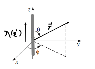
\[\vec{F} = Q\int \frac{1}{4\pi \epsilon_0}\frac{1}{|\vec{r}-\vec{r}^{\prime}|^2} \frac{\vec{r}-\vec{r}^\prime}{|\vec{r}-\vec{r}^{\prime}|}\rho dV' =QE(\vec{r})\]Then, if we have a line charge, and we are interested in $E(\vec{r})=E(z\hat{z})$ due to symmetry
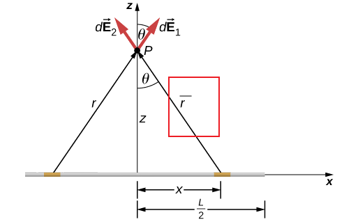
Since we only need $z$, consider $\bar{r}=\vec{r}-\vec{r}^{\prime}$ in the above figure (red box)
\[\begin{align*} \vec{E}(\vec{r}) &= \frac{1}{4\pi \epsilon_0} \int \frac{1}{\bar{r}^2}\frac{\bar{r}}{\sqrt{\bar{r}^2}}\, \rho \, dV'\\ &= \frac{1}{4\pi \epsilon_0} \int_{-L}^L \frac{1}{(z^2 + x'^2)}\frac{z\hat{z}-x'\hat{x}}{\sqrt{z^2 + x'^2}}\, \lambda \, dx'\\ \end{align*}\]essentially consider $\rho = \lambda \delta(y)\delta(z)$ since it is only on $x$-axis.
Potential when You Know $\vec{E}$
Consider the potential for a shell charge, which you already know the field:
\[\vec{E} = \begin{cases} \frac{Q}{4\pi \epsilon_0 r^2}, & r > R\\ 0, & r < R \end{cases}\]which can be proven from Gaussian surface. Then, we consider the harder potential, for $r < R$:
\[\begin{align*} V(r) &= -\int_O^r\vec{E}\cdot d\vec{l} \\ &= -\int_\infty^r \vec{E}\cdot d\vec{l}\\ &= -\int_\infty^R \vec{E}\cdot d\vec{l}-\int_R^r \vec{E}\cdot d\vec{l} \end{align*}\]then you substitute in the discontinuous field.
Conversion between Potential, Field, and Charge
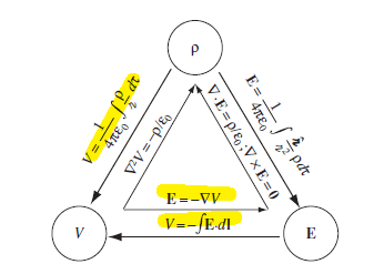
where the highlighted ones are used most often.
Induced Charges
Consider a charge neutral conductor, with $+q$ inside a cavity:
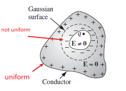
we want to show that (if the drawing above is a sphere)
\[\vec{E}_{outside} = \frac{q}{4\pi \epsilon_0}\frac{1}{r^2}\hat{r}\]which can be argued by:
-
since $\vec{E}_{meat}=0$ for conductor, we draw the Gaussian surface around the cavity to show that:
\[\oint \vec{E}\cdot d\vec{A} = 0 = \frac{Q_{enc}}{\epsilon_0}\]hence negative charges distribute at surface of cavity, such that $E_{meat}=0$ maintains
-
Then, since the negative charges effectively shielded off the $+q$, we can say that the remaining positive charge will have distributed uniformly. Hence outside the surface, we still have symmetry.
Faraday Cage:
If the cavity contains no charge inside a perfect conductor, then $\vec{E}_{\text{in cavity}}=0$
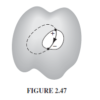
This can be shown by drawing a closed loop, so that:
- $\oint \vec{E}\cdot d\vec{l}=0$ since it is closed
- the part $\int \vec{E}\cdot d\vec{l}=0$ that covers path inside the conductor because $\vec{E}_{meat}=0$
- hence, this means $\int \vec{E}\cdot d\vec{l}=0$ for any path inside the cavity as well.
Chapter 3
Here we are concerned with finding out $V$ (hence $\vec{E}$) when we technically don’t even know $\rho$ so that:
\[V(\vec{r}) = \frac{1}{4\pi \epsilon_0} \int \frac{\rho(r')}{|\vec{r} - \vec{r}'|}d^3r'\]cannot be used.
| Condition | Equation | Comment |
|---|---|---|
| In vacuum region so that $\rho=0$ everywhere | $\nabla^2 V = 0$ | essentially solving PDE to get $V$ |
| using separation of variables | ||
| Property for $V$ that solves $\nabla^2 V=0$ | $V(\vec{r})=\frac{1}{4\pi R^2}\oint_{B_R}VdA$ | Solution of $V$ value at $\vec{r}$ is the average of surrounding (mean value theorem) |
| (follows from the above) Extremum for $V$ only happens at the boundary | ||
| Earnshaw’s Theorem | A charged particle cannot be held in stable equilibrium by electrostatic force | If stable equilibrium, $V(r_{eq}) > V(r_{surface})$ for a ball of radius $R$ around it. |
| But since $\nabla^2V=0$ holds, then from MV theorem this cannot be true. | ||
| Uniqueness Theorem | Solution to $\nabla^2V=0$ is unique | Proven by $V_3 = V_2 - V_1$, and showing that $V_3=0$ is a must if $V_1,V_2$ solves both PDE and boundary condition |
| Solution to $\nabla^2V = - \rho / \epsilon_0$ is also unique | same idea as above | |
| Method of Images | Figuring out $V$ is the same as solving $\nabla^2V=0$ with boundary condition. Use method of images to satisfy B.C. while making sure $\rho = 0$ in the interested region. | |
| Works because of uniqueness theorem | ||
| Useful when you don’t want to actually solve $\nabla^2V=0$ | ||
| 2D Cartesian Solution for Laplacian | $V(x,y)=(Ae^{kx}+Be^{-kx})(C\sin(ky)+D\cos(ky))=X(x)Y(y)$ | General Solution, $k$ needs to be solved by looking at B.C. |
| $k=n \pi /a$, solution $V(x,y) = \sum_n V_n(x,y)$ | sometimes you can tell what $n$ should be, e.g. $n=5$. Then solution is simply one term of the sum | |
| 2D Cylindrical Solution for Laplacian | $\nabla^2V = \frac{1}{r}\frac{\partial }{\partial r}(r \frac{\partial V}{\partial r})+\frac{1}{r^2}\frac{\partial^2 V}{\partial \phi^2}=0$ | |
| $V(r,\phi) = (Ar^m + Br^{-m})(C\sin(m\phi)+D\cos(m\phi))$ | General solution, $m$ needs to be solved by looking at B.C. | |
| 3D Spherical Solution without horizontal $\phi$ | $\nabla^2 V = \frac{1}{r}\frac{\partial }{\partial r^2}(r^2 \frac{\partial V}{\partial r})+\frac{1}{r^2 \sin(\theta)}\frac{\partial^2 V}{\partial \theta^2}=0$ | |
| $V(r,\theta, \phi)=(Ar^l + \frac{B}{r^{l+1}})P_l[\cos(\theta)]$ | ||
| Legendre Polynomial | $P_0[\cos(\theta)]=1 \ P_1[\cos(\theta)]=\cos \theta \ P_2[\cos(\theta)]=(3\cos^2 \theta -1)/2$ | Good to remember |
| $\int_0^\pi P_i[\cos(\theta)]P_j[\cos(\theta)]\sin(\theta) \, d\theta = \begin{cases} 0, & i \neq j\ \frac{2}{2i+1}, & i = j \end{cases}$ | Orthogonality, use for non-homogenous boundary condition (if needed) | |
| Multipole Expansion | $V(\vec{r}) = \frac{1}{4 \pi \epsilon_0} \sum_{l=0}^\infty \frac{1}{r^{l+1}} \int (r’)^l P_l[\cos(\theta)] \rho(r’)d^3r’$ | Approximation useful when we are far away. Proof from $V(\vec{r}) = \frac{1}{4 \pi \epsilon_0}\int \frac{\rho(r’)}{\vert \vert \vec{r}-\vec{r}’‘\vert \vert } d^3r’$ and using result below |
| $\frac{1}{\vert \vert \vec{r}-\vec{r}’\vert \vert } = \frac{1}{r}\sum_l^\infty \left( \frac{r’}{r} \right)^l P_l[\cos(\theta)]$ | for $r = \vert \vert \vec{r}\vert \vert , r’=\vert \vert \vec{r}’\vert \vert$, proven from binomial expansion of denominator taking out $R$. | |
| $V(\vec{r}) = \frac{1}{4 \pi \epsilon_0}\sum_{l=0}^\infty \frac{M_l}{r^{l+1}}P_l[\cos\theta]$, $M_l \equiv \int (r’)^l \rho(r’)d^3r’$ | assuming $P_l[\cos\theta]$ can be taken out from the integral | |
| $V_l = \frac{1}{4\pi \epsilon_0} \frac{M_l P_l[\cos\theta]}{r^{l+1}}$, so $V(\vec{r}) = \sum_{l=0}^\infty V_l$ | e.g. monopole potential take $l\to 0$, dipole potential take $l \to 1$, quadruple potential take $l\to 2$,… | |
| Multipole Terms | $M_l \equiv \int (r’)^l \rho(r’)d^3r’$ | in continous case |
| $M_l \equiv \sum_i (r_i’)^l q_i$ | in discrete case (both assume $\theta$ being a constant, otherwise $P_l[\cos \theta]$ will be included) | |
| $V_l = \frac{1}{4\pi \epsilon_0} \frac{M_l P_l[\cos\theta]}{r^{l+1}}$ | ||
| Dipole Moment | $V_1(\vec{r}) = \frac{1}{4 \pi \epsilon_0} \frac{1}{r^{2}} \int r’ \cos(\theta )\rho(r’)d^3r’ = \frac{1}{4\pi \epsilon_0} \frac{1}{r^2} \int \hat{r}\cdot \vec{r}’ \rho(r’)d^3r’$ | |
| $V_1(\vec{r}) = \frac{1}{4\pi\epsilon_0}\frac{1}{r^2}\hat{r}\cdot \vec{p}$, with $\vec{p} \equiv \int \vec{r}’ \rho(r’)d^3r’$ | Dipole Moment $\vec{p}$ without any assumption | |
| $\vec{p} = \sum_i \vec{r}’_i q_i$ | Dipole Moment in discrete case |
Method of Imaging
Consider finding $V$ in the following region where $z > 0$:
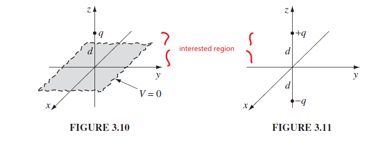
Notice that finding out $V$ in that region is the same as:
- solving $\nabla^2 V=0$
- B.C.: $V=0$ when $z=0$ as it is grounded
- B.C.: $V(r)\to 0$ if $r^2 » d^2$, i.e. when far away
- $\vec{E}$ is perpendicular to surface at $z=0$
- good check to make sure if method of imaging setup is correct
Then, realize that this is the same as solving for $V$ in Figure 3.11.
- in the end we only take the solution for $z>0$
Since it is essentially two point charges, use superposition of potential from point charges:
\[V(x,y,z) = \frac{1}{4\pi \epsilon_0} \left[ \frac{q}{\sqrt{x^2 + y^2 + (z-d)^2}} -\frac{q}{\sqrt{x^2 + y^2 + (z+d)^2}} \right]\]Multipole Expansion Derivation Sketch
This comes from the motivation to approximate field when we are far from the charge density. Technically the approximation
\[V(\vec{r}) \approx \frac{1}{4\pi \epsilon_0} \frac{Q_{total}}{r^2}\]could work in some cases, in other case you might have $Q_{total}=0$ then this is uninformative, i.e. we need higher order terms. Hence we first use binomial expansion to show that:
\[\frac{1}{||\vec{r}-\vec{r}'||} = \frac{1}{r}\sum_l^\infty \left( \frac{r'}{r} \right)^l P_l[\cos(\theta)]\]from doing
\[\frac{1}{||\vec{r}-\vec{r}'||} = \frac{1}{\sqrt{r^2 + r^{'2}-2rr'\cos \theta}} = \frac{1}{r}\frac{1}{\sqrt{1+\epsilon}}\]then expanding the $1/\sqrt{1+\epsilon}$ to get Legendre polynomial, which assumes small $\epsilon$ hence being far away from charges.
Multipole Expansion Example
Consider a vertical line charge $\lambda (z’)$, and we are interested in finding $V(\vec{r})$ far away from it.
Using the formula for expansion, we know:
\[V(\vec{r}) = \frac{1}{4 \pi \epsilon_0} \sum_{l=0}^\infty \frac{1}{r^{l+1}} \int (r')^l P_l[\cos(\theta)] \rho(r')d^3r'\]then since $\rho(r’) = \lambda(z’)\delta(x’)\delta(y’)$, and since $\vec{r}’ = z’\hat{z}$, meaning $r’=z’$, then we get:
\[\begin{align*} V(\vec{r}) &= \frac{1}{4 \pi \epsilon_0} \sum_{l=0}^\infty \frac{1}{r^{l+1}} \int (z')^l P_l[\cos \theta] \lambda(z')\delta(x')\delta(y')\,d^3r'\\ &= \frac{1}{4 \pi \epsilon_0} \sum_{l=0}^\infty \frac{P_l[\cos\theta]}{r^{l+1}} \iiint (z')^l \lambda (z')\delta(x')\delta(y')\,dx'dy'dz'\\ &= \frac{1}{4 \pi \epsilon_0} \sum_{l=0}^\infty \frac{P_l[\cos\theta]}{r^{l+1}} \int (z')^l \lambda (z')dz' \end{align*}\]which is the furthest we can go, and the second equality comes from the fact that $\theta$ which is the angle between $\vec{r}$ and $\vec{r}’$ is constant given a $\vec{r}$.
Multipole Expansion Discrete case:
If you are dealing with a discrete case, you can then either:
-
express $\rho(\vec{r}’)$ in terms of $\delta$ functions, hence point charges
-
use the discrete formula for $M$. Since we assumed to be far away from the charges, usually $\theta_i$ between $\vec{r}$ and $\vec{r}_i’$ can be assumed constant hence:
\[V(\vec{r}) = \frac{1}{4 \pi \epsilon_0}\sum_{l=0}^\infty \frac{M_l}{r^{l+1}}P_l[\cos\theta], \quad M_l \equiv \sum_i (r_i')^l q_i\]otherwise you will need:
\[V(\vec{r}) = \frac{1}{4 \pi \epsilon_0}\sum_{l=0}^\infty \frac{M_l}{r^{l+1}}, \quad M_l \equiv \sum_i (r_i')^l \, P_l[\cos\theta_i] \, q_i\]
Chapter 4
This chapter discuss electric fields in matter (e.g. dielectric), which is what happens when an electric field $\vec{E}_{app}$ is applied on the matter.
| Condition | Equation | Comment |
|---|---|---|
| Atomic Polarization | $\vec{p} = \alpha \vec{E}_{applied}$ | For molecules, $\alpha$ would be a function of “direction” if molecule is asymmetric (e.g. $H_2O$) |
| Polarization | $\vec{P}$=dipole moment per volume | describes polarization of material due to some externel field |
| $\vec{p} = \vec{P}\,dV’$ | Want to find field results from polarization $\vec{P}$ | |
| $\vec{P}(\vec{r}’)=0$ if $\vec{r}’$ is vacuum, for example | ||
| Potential due to Polarization $\vec{P}$ | $V(\vec{r}) = \frac{1}{4\pi \epsilon_0} \oint_\Omega \frac{\sigma_b}{\vert \vert \vec{r} - \vec{r}’\vert \vert }dA’+ \frac{1}{4\pi \epsilon_0} \int_V \frac{\rho_b}{\vert \vert \vec{r} - \vec{r}’\vert \vert }dV’$ | derived from $V(\vec{r})$ only consisting of dipole terms, which is defined by $\vec{P}(\vec{r})$ |
| $V(\vec{r})=V(\text{from$\sigma_b, \rho_b$})$ | i.e. you can treat the dielectric as having $\sigma_b$ on the surface and $\rho_b$ inside. | |
| if $\rho_b = 0$, $V(\text{from$\sigma_b,\rho_b$})$ can be solved using Laplacian $\nabla^2 V = 0$ with boundary of $\sigma_b$ | ||
| $\sigma_b \equiv \vec{P}\cdot \hat{n}$ | $\hat{n}$ points from the surface having dielectric to vaccum/non-dielectric place | |
| $\rho_b\equiv - \nabla \cdot \vec{P}$ | ||
| Interpretation of Bound Charge due to $\vec{P}$ | $\sigma_b \equiv \vec{P}\cdot \hat{n}$ | $\sigma_b$ comes from lining up dipoles so that only ends matter |
| $\rho_b\equiv - \nabla \cdot \vec{P}$ | $\rho_b$ considers if dipole in between is not cancelled out, then the flux of polarization would relate to charge: $-\oint \vec{P}\cdot d\vec{A} =\int_V \rho_b \,d^3r’$ | |
| Electric Displacement Field | $\vec{\nabla} \cdot \vec{D}= \rho_{free}$, and $\vec{D} \equiv \epsilon_0 \vec{E}_{total} + \vec{P}$ | differential form |
| $\vec{\nabla}\cdot \vec{E}{tot} = \frac{\rho{free}+\rho_b}{\epsilon_0}$ | derivation, then using $\rho_b = -\vec{\nabla}\cdot \vec{P}$ | |
| $\oint \vec{D}\cdot d\vec{A} = Q_{free_{enc}}$ | integral form | |
| if have symmetry can use Gaussian surfaces | ||
| used for proving boundary conditions for $\vec{D}$ | ||
| $\vec{\nabla} \times \vec{D} = \vec{\nabla} \times \vec{P}$ | ||
| $\oint \vec{D}\cdot d\vec{r}=\oint \vec{P}\cdot d\vec{r}$ | Stokes’ Theorem, derived from above | |
| used for proving boundary conditions for $\vec{D}$ | ||
| the above is true for any dielectric | ||
| $\vec{D}$ and $\vec{E}$ relation | $\vec{\nabla}\cdot \vec{E}{tot} = \rho{tot} / \epsilon_0 \to \vec{E}{tot} = \frac{1}{4\pi \epsilon_0} \int \frac{\rho{tot}}{\symscr{r}} \hat{\symscr{r}}\,d^3r’$ | because $\vec{\nabla}\times \vec{E}_{tot} = 0$ |
| $\vec{\nabla}\cdot \vec{D}= \rho_{free} \not\to \vec{D} = \frac{1}{4\pi } \int \frac{\rho_{free}}{\symscr{r}} \hat{\symscr{r}}\,d^3r’$ | because $\vec{\nabla} \times \vec{D} \neq 0$ often, hence $\vec{D}$ might not have a potential | |
| Linear Dielectric | $\vec{P} = \epsilon_0 \chi_e \vec{E}_{tot}$ | $\chi_e$ is electric susceptibility, $\epsilon_0$ is permittivity of free space |
| if $\vec{E}{applied}$ is given, we are stuck because it will produce $\vec{P}$, which produces $\vec{E}{resp}$ hence affects $\vec{E}_{tot}$, which relates to $\vec{P}$… | ||
| $\vec{D} = \epsilon_0(1+\chi_e)\vec{E}{tot}\equiv \epsilon \vec{E}{tot}$ | $\epsilon$ is permittivity of material | |
| can use this to break from the loop if we can find $\vec{D}$ from Gaussian surface | ||
| $\epsilon_r \equiv \epsilon / \epsilon_0 = 1+\chi_e$ | relative permittivity, $\chi_e=0$ in free space. | |
| also called dielectric constant | ||
| $\vec{\nabla}\times \vec{D} = \vec{\nabla} \times (\epsilon \vec{E}_{tot}) \neq 0$ | because $\epsilon$ could vary in different position | |
| Space filled with homogenous Linear Dielectric $\chi_e$ | $\vec{\nabla} \times \vec{D} = 0$, $\vec{\nabla} \cdot \vec{D}= \rho_{free}$ | inside the homogenous linear dielectric, $\epsilon$ is constant |
| $\vec{D} = \epsilon_0 \vec{E}_{free}$ | $\vec{E}_{free}$ is field produced by free charges | |
| because now $\vec{\nabla}\cdot \vec{D}= \rho_{free} \to \vec{D} = \frac{1}{4\pi } \int \frac{\rho_{free}}{\symscr{r}} \hat{\symscr{r}}\,d^3r’$ holds | ||
| Happens when $\vec{\nabla} \times\vec{D} = \vec{\nabla} \times\vec{P}= 0$, commonly with a capacitor | $\vec{E}{tot} = \frac{1}{\epsilon_r}\vec{E}{free}\equiv \frac{1}{\epsilon_r}\vec{E}_{vac}$ | for capacitor: derived if $\vec{D}$ has the same shape as $\vec{E}{vac}$ , then use Gaussian to find $\vec{D}$ and use $\vec{D} = \epsilon \vec{E}{tot}$ |
| in general, $\vec{\nabla} \times\vec{D} = 0$ alone would work. See the relevant section below | ||
| note that this is a special case on top of having a linear dielectric | ||
| Boundary Conditions for $\vec{D}$ | $D_{abv}^\perp - D_{below}^\perp = \sigma_{free}$ | derived from drawing Gaussian box just above/below the surface |
| $D_{abv}^\parallel - D_{below}^\parallel= P_{abv}^\parallel - P_{below}^\parallel$ | derived from drawing loop just above/below the surface | |
| True for any dielectric | ||
| $\vec{E}{above}-\vec{E}{below} = (\sigma_{total}/\epsilon_0) \hat{n}$ | (note that those always/still hold) | |
| $E_{abv}^\parallel - E_{below}^\parallel= 0$ | ||
| Dielectric inside Capacitor | $C = \epsilon_r C_{vac}$ | $C_{vac}$ is capacitance without dielectric |
| holds whenever $\vec{E}{tot} = \frac{1}{\epsilon_r}\vec{E}{free}$ holds inside the capacitance. Hence $\Delta V = \Delta V_{vac}/\epsilon_r$ while $Q$ is the same. | ||
| Energy of setup with a Dielectric | $W=\frac{1}{2}\int_{all\,space}\vec{D}\cdot\vec{E}\,d^3r$ | holds if you have a linear dielectric so that $\vec{D}=\epsilon \vec{E}$ |
| derived from assuming bound charges fixed in place, we are only moving free charges into position | ||
| $W = \frac{\epsilon_0}{2}\int \vert \vec{E}\vert ^2 d^3r$ | still holds if we are assembling all charges independently, i.e. we also bring in bound charges | |
| this will be smaller than $W=\frac{1}{2}\int_{all\,space}\vec{D}\cdot\vec{E}\,d^3r$ as it does not include potential/spring energy within dipoles | ||
| Force on Dielectric (due to capacitor) | $-F_{on\,diel}=\frac{dW}{dx}=-\frac{1}{2}V(x)^2\frac{dC(x)}{dx}$ | True either fixing $Q$ or fixing $V$, in which case $V(x)=V_0$ |
| sanity check: force should suck dielectric into capacitor | ||
| $dW = F_{me}dx=-F_{on\,diel}dx$, and $W=\frac{1}{2}\frac{Q^2}{C(x)}$ | derivation. For $C(x)$ and $V=V(x)$ if fixed total charge $Q$ | |
| $dW=-F_{on\, diel}dx + VdQ$, and $W=\frac{1}{2}C(x)V_0^2$ | derivation if fixing $V(x)=V_0$. Ended up the same formula for $W$ as above. | |
| $\vec{\nabla} W = -\vec{F}_{on\, diel}$ | If in problem we have some 3D movement. Then $W$ is still one of the two above cases. |
Atomic Polarization
This is derived/approximated by considering the nucleus with charge $+q$ sits in equilibrium due to cancellation of external field $\vec{E}_{app}$ and $\vec{E}_e$ with is field of electron cloud (volume):
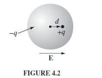
Then since field inside uniform sphere of charge is:
\[\vec{E}_e = -\frac{q}{4\pi \epsilon_0} \frac{r}{a^3} \hat{r},\quad r<a\]hence if we obtained an equilibrium at $r=d$:
\[\begin{align*} \vec{E}_{app}(d) &=\frac{q}{4\pi \epsilon_0} \frac{d}{a^3} \hat{r}\\ qd \hat{r} \equiv \vec{p} &= (4\pi \epsilon_0 a^3)\vec{E}_{app}(d) \end{align*}\]hence the proportionality.
Application of Bound Charges
Consider a slab of dielectric with thickness $d$ carrying polarization $\vec{P} = k[1+(x/d)]\hat{x}$ :
we do not care yet what external field is needed to produce this polarization. We want to know the electric field produced by this given polarization.
First, we can find the bound charges to be:
\[\sigma_b = \vec{P}\cdot \hat{n} = \begin{cases} 2k, & x =d\\ -k, & x=0 \end{cases}\\ \rho_b = -\nabla \cdot \vec{P} = -\frac{k}{d},\quad 0<x<d\]Then, we can treat this as real charges to compute $V(\vec{r})$ due to the correctness of:
\[V(\vec{r}) = \frac{1}{4\pi \epsilon_0} \oint_\Omega \frac{\sigma_b}{||\vec{r} - \vec{r}'||}dA'+ \frac{1}{4\pi \epsilon_0} \int_V \frac{\rho_b}{||\vec{r} - \vec{r}'||}dV'\]Now, since we know the charge distribution, we can exploit the symmetry and save doing the above extra integrals:
-
drawing Gaussian surfaces inside/outside the slab gives:
\[\vec{E}_< = \vec{E}_>\\ (\vec{E}_{inside}-\vec{E}_{<})\cdot \hat{x} = \frac{k}{\epsilon_0}\left(1+\frac{x}{d}\right)\] -
but notice that the net charge is zero, hence:
\[\vec{E}_< = \vec{E}_> = \vec{0}\\ \vec{E}_{inside} = -\frac{k}{\epsilon_0}\left( 1+ \frac{x}{d} \right)\]
the result is consistent if you compute from $\vec{D}$ and use $\vec{D}=\epsilon \vec{E}_{tot}$.
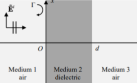
Homogenous Linear Dielectric:
Find $\vec{E}_{tot}$ inside the dielectric with the following setup, $Q$ is free charge placed by us.
First, a linear dieletric means $\vec{D} = \epsilon \vec{E}{tot}$. Then, as $\epsilon$ is constant inside, we get $\vec{\nabla} \times\vec{D} = 0$. Then $\vec{\nabla}\cdot \vec{D}= \rho{free}$ always hold, we can use:
\[\vec{D} = \frac{1}{4\pi } \int \frac{\rho_{free}}{\symscr{r}} \hat{\symscr{r}}\,d^3r'\]meaning that:
\[\vec{D} = \epsilon_0 \vec{E}_{free},\quad \vec{E}_{tot} = \frac{1}{\epsilon_r}\vec{E}_{free}\]since inside the dielectric we have $\vec{E}_{free} = q/(4\pi \epsilon_0 r^2) \hat{r}$, our final answer is:
\[\vec{E}_{tot}^{inside} = \frac{1}{\epsilon_r} \left( \frac{q}{4\pi \epsilon_0 r^2} \right)\hat{r}\]which is intuitive because:
- dielectric getting polarized = induced dipole opposes $\vec{E}{app}$, hence $\vec{E}{tot}^{inside}$ becomes smaller
- if conductor, then $\epsilon_r \to \infty$ since $\chi_e \to \infty$. Then naturally $\vec{E}_{tot}^{inside}=0$ inside conductor
(can verify this result by starting with drawing Gaussian surface for finding $\vec{D}$)
Treating $\sigma_b,\rho_b$ as real charges:
Basically it works due to the proof that
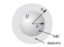
\[V(\vec{r}) = \frac{1}{4\pi \epsilon_0} \oint_\Omega \frac{\sigma_b}{||\vec{r} - \vec{r}'||}dA'+ \frac{1}{4\pi \epsilon_0} \int_V \frac{\rho_b}{||\vec{r} - \vec{r}'||}dV'\]Then, consider finding $V(r)$ for $r < a$ in the setup below:
where $Q$ is a point charge sitting at origin. Then, we first can easily figure out $\vec{D}$ by:
\[\int \vec{D}\cdot d\vec{S} = Q_{free_{enc}} = Q,\quad \text{true for all space}\]hence we get:
\[\vec{D} = \frac{Q}{4 \pi r^2}\hat{r}\to \vec{E}_{tot} = \frac{Q}{4\pi \epsilon r^2}\hat{r}\]for $\epsilon$ actually changes in regions, so that:
- $\epsilon=\epsilon_0$ in vacuum hence $r < a$ or $r > b$
- $\epsilon =\epsilon_r \epsilon_0$ inside dielectric
Though we can proceed easily to find $V(\vec{r})$ now, but we can show that we obtain the same result if we treating $\sigma_b,\rho_b$ as real charges:
-
to find $\sigma_b, \rho_b$, first we need to find $\vec{P}$:
\[\vec{P} = \epsilon_0 \chi_e \vec{E}_{tot} = \frac{\epsilon_0 \chi_e Q}{4\pi \epsilon r^2}\hat{r}\] -
then find $\sigma_b, \rho_b$:
\[\sigma_b =\vec{P}\cdot \hat{n} = \begin{cases} -\frac{\epsilon_0 \chi_e Q}{4\pi \epsilon a^2} , & x =a\\ \frac{\epsilon_0 \chi_e Q}{4\pi \epsilon b^2} , & x =b \end{cases}\\ \rho_b = -\nabla \cdot \vec{P} =0,\quad a<x<b\]
Then we can consider $\vec{E}_{tot}$ from those charges while using symmetry:
\[\begin{cases} \vec{E}_{<} = \frac{Q}{4 \pi \epsilon_0 r^2} \hat{r}, & r < a\\ \vec{E}_{inside} = \frac{Q+Q_b(a)}{4 \pi \epsilon_0 r^2} \hat{r}= \frac{Q}{4 \pi \epsilon_0(1+\chi_e) r^2} \hat{r}, & a<r <b\\ \vec{E}_{>} = \frac{Q}{4 \pi \epsilon_0 r^2} \hat{r}, & r > b \end{cases}\]using $\oint \vec{E}\cdot d\vec{A} = Q_{enc}/\epsilon_0$, where:
- $Q_b(a)$ is the bound charges at $r=a$, which is $4 \pi a^2 \sigma_b(a)$.
- this is consistent with $\vec{E}_{tot} = \frac{Q}{4\pi \epsilon r^2}\hat{r}$.
Finally, finding $V(\vec{r})$ for $r < a$ is just doing the integral:
\[V(\vec{r}) = -\int_\infty^r \vec{E}\cdot d\vec{r} = -\int_\infty^b \vec{E}_<\cdot d\vec{r}-\int_b^a \vec{E}_{inside}\cdot d\vec{r}-\int_a^r \vec{E}_>\cdot d\vec{r}\]for $d\vec{r}=dr \hat{r}+ rd\theta \hat{\theta}$.
Application of Force on Dielectric
In most cases the force is only in one direction, hence using this suffices:
\[-F_{on\,diel}=\frac{dW}{dx}=-\frac{1}{2}V(x)^2\frac{dC(x)}{dx}\]Consider the setup of
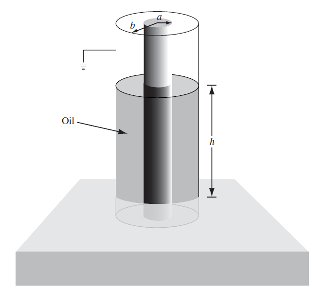
where oil is the dielectric, with $\chi_e$ and $\rho_{oil}$. Here we assume the inner conductor is fixed on $V=V_0$, and the outer is grounded. We want to know the height of oil at equilibrium = at what $z$ we have $F_{on\,diel}$ cancels $F_{g}$
No matter fixing $V$ or fixing $Q$, we still have
\[-F_{on\,diel}=\frac{dW}{dz}=-\frac{1}{2}V(z)^2\frac{dC(z)}{dz}=-\frac{1}{2}V_0^2\frac{dC(z)}{dz}\]Hence we just need to find out $C(z)$. Since $\Delta V=V_0$ is fixed, hence we just need to find out $Q(z)$ as we know:
\[C(z) = \frac{Q(z)}{\Delta V}=\frac{Q(z)}{V_0}\]If we consider charges as line density $\lambda \cdot l$, then we know
\[Q(z) = \lambda_{diel}z + \lambda_{vac}(l-z)\]Then $\lambda_{vac}$ can be easily calculated from $E_{vac}=V_0/(b-a)$ and using a Gaussian surface. Finding $\lambda_{diel}$ is similarly doing
\[\int \vec{D}\cdot d\vec{S}=2\pi r l D=\lambda_{diel}l\quad \to \quad \vec{D} = \frac{\lambda_{diel}}{2\pi r}=\epsilon \vec{E}_{diel}\]Since we need $V_0$ to hold everywhere, we then can solve $\lambda_{diel}$:
\[|\vec{E}_{diel}|\cdot (b-a)=|\vec{E}_{vac}|\cdot (b-a)\quad \to \quad \lambda_{diel}=\epsilon_r \lambda_{vac}\]which is a common result as we always had $\sigma_{diel}=\epsilon_r \sigma_{vac}$ whenever $\vec{D}$ and $\vec{E}$ has a similar shape + symmetry.
Chapter 5
Electrostatics studies essentially the force on some test charge $Q$ due to some static source charges $\rho(\vec{r})$.
Magnetostatics studies the force on some moving test charge $Q, v$, due to mangetic field produced by steady source current $J = \rho v$. The important difference between magnetostatics and electrostatics is:
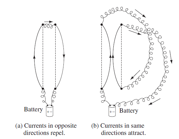
the wires are still charge neural hence no net electric field, but there is magnetric field due to moving charges and hence Lorentz force appears! Therefore, this chapter discusses
- motion due to Lorentz force (e.g. cycltron motion)
- how to compute $\vec{B}$ in different scenarios (e.g. using $\vec{\nabla} \times \vec{A} = \vec{B}$)
| Condition | Equation | Comment |
|---|---|---|
| Force due to $B$ | $\vec{F}_{mag}= Q(\vec{v}\times \vec{B})$ | experienced by charge $Q$ moving with velocity $\vec{v}$ |
| $\vec{F}_{total}=Q(\vec{E}+\vec{v}\times \vec{B})$ | if there is also an electric field | |
| Current | $I = dq/dt$ | Useful for deriving $I$ when given 3D shapes |
| $I = \lambda v$ | for currents since $dq = \lambda dl$ | |
| for instance, $dq = \rho dV=\rho Adl$ | ||
| assumes it is the direction of positive charges moving | ||
| Force due to B on a current wire | $\vec{F}_{mag} = I \int d\vec{l}\times \vec{B}$ | For wire essentially it is a collection of moving charges with $dq= \lambda dl$ |
| $d\vec{F}_{mag} = dq(\vec{v}\times \vec{B}) = \lambda dl(\vec{v}\times \vec{B})=(\vec{I}\times \vec{B})dl$ | derivation of the above | |
| basically still Lorentz force | ||
| Work done by $B$ | $dW_{mag} = \vec{F}_{mag}\cdot{d\vec{l}}=0$ | Because $\vec{F}_{mag}= Q(\vec{v}\times \vec{B})$ but $d\vec{l}= \vec{v}dt$ |
| Therefore, it only changes direction of velocity | ||
| Charge density | $J = \rho v = dI/da_{\perp}$ | The parallel of $\rho$ in electrostatstics |
| Used for Biot-Savart Law | ||
| $I = \int \vec{J} \cdot d\vec{S}$ | current in a wire with $\vec{J}$ | |
| Force due to $B$ on a current density | $\vec{F}_{mag} = \int \vec{J}\times \vec{B}d\tau$ | essentially it is a collection of moving charges with $dq= \rho d\tau$ |
| $d\vec{F}_{mag} = \rho d\tau (\vec{v}\times \vec{B}) =(\vec{J}\times \vec{B})d\tau$ | ||
| Cycltron Drift Velocity | $\vec{v}_{drift} = \frac{\vec{E}\times \vec{B}}{B^2}$ | a moving charge then there is both $E$ and $B$ field, it drifts in addition to looping |
| better to find this during solving ODEs | ||
| Cycltron Rotation Frequency | $w_c = \vert qB/m\vert$ | found by solving the ODE |
| Cycltron Radius | $R = (mv) / (qB)$ | because $R = v/\omega_c$ for $v$ being the orbital speed |
| works if we are only rotating | ||
| Biot-Savart Law Generic | $\vec{B}(\vec{r}) = \int \frac{\mu_0}{4\pi} \frac{\vec{J}(\vec{r}’)\times(\vec{r}-\vec{r’})}{\vert \vec{r}-\vec{r’}\vert ^3}\,d^3r’$ | True if $J$ is independent of time, i.e. steady |
| $\vec{E}(\vec{r}) = \int \frac{1}{4\pi \epsilon_0} \frac{\vec{\rho}(\vec{r}’)\cdot(\vec{r}-\vec{r’})}{\vert \vec{r}-\vec{r’}\vert ^3}\,d^3r’$ | parallel to the $\vec{E}$ field, basically $J \to \rho$ | |
| $\mu_0 = 1/(\epsilon_0 c^2)$ | ||
| Biot-Savart if Steady current | $\vec{B}(\vec{r}) = \frac{\mu_0 I}{4\pi} \int \frac{d\vec{l}(\vec{r}’)\times(\vec{r}-\vec{r}’)}{\vert \vec{r}-\vec{r}’\vert ^3}$ | basically we have here $\vec{J} = \vec{I}\delta^2(\vec{r}-\vec{r}’)$ and that $\vec{I}dl = Id\vec{l}$ |
| works if constant current so $\vec{I}dl = Id\vec{l}$ holds | ||
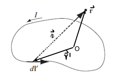 |
Integrates $dl’$ only over where $\vec{r}’ \neq 0$ | |
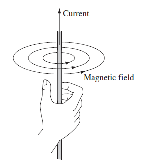
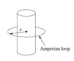
| Magnetric Field of a Straight line wire | $\vec{B} = \frac{\mu_0 I}{2\pi r} \hat{e}_\phi$ | Found either using Biot-Savart for current, or using the symmetry hence $\oint \vec{B}\cdot d\vec{l} = \mu_0 I_{enc}$ |
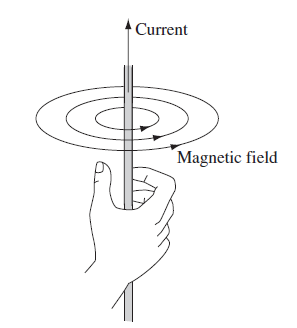 |
Graphically it circulates the current | |
| Divregence of B | $\vec{\nabla}_{\vec{r}} \cdot \vec{B}(\vec{r})=0$ | for E field we had $\vec{\nabla}\cdot \vec{E}= \rho/\epsilon_0$ |
| $\oint \vec{B}\cdot d\vec{S}=0$ | for E field we had Gaussian surface $\oint \vec{E}\cdot d\vec{S}=Q_{enc}/\epsilon_0$! | |
| derived using $\int \vec{\nabla}\cdot\vec{B} d\tau = \oint \vec{B}\cdot d\vec{S}$ | ||
| not very useful for B field calculation | ||
| Curl of B | $\vec{\nabla}_{\vec{r}} \times \vec{B}(\vec{r})=\mu_0 \vec{J}(\vec{r})$ | for E field we had this is 0 |
| $\oint \vec{B}\cdot d\vec{l}=\mu_0 I_{enc}$ | very useful for B field calculation if we have symmetry in $J$ or $I$ setup! | |
| called Ampere Loops | ||
| derived using $\int \vec{\nabla}\times \vec{B}\cdot d\vec{S} = \oint \vec{B}\cdot d\vec{l}$ | ||
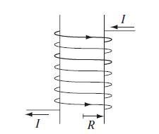
| Field of Solenoid with $n$ turns per unit legnth | $\vec{B} = \mu_0 n I \hat{e}_z$ | if inside the solenoid |
| $\vec{B}=0$ | if outside | |
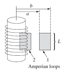 |
Essentially solved by drawing Amphere loops | |
| Magnetic Vector Potential | $\vec{\nabla}\times \vec{A} = \vec{B}$ | so that $\vec{A}$ is easier to compute |
| from $\vec{E}= - \vec{\nabla}V$ for $V$ is easier to compute | ||
| Gauges for $\vec{A}$ due to above definition | $\nabla(\nabla \cdot \vec{A})-\nabla^2\vec{A} = \mu_0 \vec{J}$ | if $\vec{\nabla}\times \vec{A} = \vec{B}$, and we know $\nabla \times \vec{B} = \mu_0 \vec{J}$ |
| if $\nabla \cdot \vec{A} = 0$ | Colomb’s Gauge, used by this course | |
| $\vec{A}’ = \vec{A}+ \nabla\lambda$ results in the same $B$ field | therefore we can always force $\nabla \cdot \vec{A} = 0$ by choosing $\lambda$ | |
| Magnetic Vector Potential Definition | $\vec{A} = \frac{\mu_0}{4\pi}\int \frac{\vec{J}(\vec{r}’)}{\vert \vec{r}-\vec{r}’\vert }d^3r’$ | derived from the above with $\nabla^2 \vec{A}=-\mu_0 \vec{J}$, so that each compontent $A_x,A_y,A_z$ essentially is an analog version of $\nabla^2 V = - \rho / \epsilon_0$ and we know the solution $V$ from using $\rho$ |
| this means that $\vec{A}$ is usually in the same direction as current! | ||
| Technically $\vec{A} = \frac{\mu_0}{4\pi}\int \frac{\vec{J}(\vec{r}’)}{\vert \vec{r}-\vec{r}’\vert }d^3r’ + \vec{A}(0)$ | for $\vec{A}(0)$ is a reference point | |
| usually use $\vec{A}(\infty)=0$ | ||
| Flux (open surface) | $\Phi \equiv \int \vec{B}\cdot d\vec{A} = \oint \vec{A}\cdot d\vec{l}$ | non-zero because this is an open surface |
| don’t confuse against $\oint \vec{B}\cdot$ | ||
| can be used to find $\vec{A}$ if we have symmetry and knows $\vec{B}$ | ||
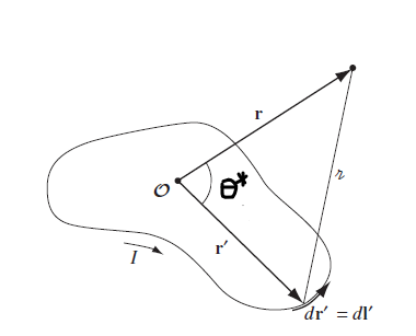
| Multipole Expansion of $\vec{A}$ | $\vec{A}(\vec{r}) = \frac{\mu_0}{4\pi}\sum_{n=0}^\infty \frac{1}{r^{n+1}}\int \vec{J}(\vec{r}’)(r’)^n P_n[\cos \theta^*]d^3r’$ | we can no longer take $P_n[\cos \theta^]$ for $\theta^$ is the angle between $\vec{r}, \vec{r’}$ over any shaped wire! |
| derivation is simply the same as electrostatic case, taking $\frac{1}{\vert \vec{r}-\vec{r}’\vert }=\frac{1}{r}\sum_{n}^\infty (\frac{r’}{r})^n P_n[\cos \theta^*]$ | ||
| $\vec{A}(\vec{r})=\frac{\mu_0}{4\pi}\sum_{n=0}^\infty \frac{M_n}{r^{n+1}}$, for $M_n=\int \vec{J}(\vec{r}’)(r’)^n P_n[\cos \theta^*]d^3r’$ | $n$-th Moment term | |
| $V(\vec{r}) = \frac{1}{4 \pi \epsilon_0}\sum_{l=0}^\infty \frac{M_l}{r^{l+1}}P_l[\cos\theta]$, $M_l \equiv \int (r’)^l \rho(r’)d^3r’$ | electrostatic case where $\theta^*=\theta=\text{const}$ | |
 |
Grahpically we we are doing | |
| Generic and true if far away | ||
| Multipole Expansion of $\vec{A}$ with a wire | $\vec{A}(\vec{r}) = \frac{\mu_0 I}{4\pi}\sum_{n=0}^\infty \frac{1}{r^{n+1}}\int (r’)^n P_n[\cos \theta^*]d\vec{l}’$ | Using $\vec{J} = \vec{I}\delta^2(\vec{r}-\vec{r}’)$ and then $\vec{I}dl = Id\vec{l}$ |
| $\vec{A}(\vec{r})=\frac{\mu_0}{4\pi}\sum_{n=0}^\infty \frac{M_n}{r^{n+1}}$, for $M_n=\int I(r’)^n P_n[\cos \theta^*]d\vec{l}’$ | $n$-th Moment term | |
| use this if we have a wire with current $I$ | ||
| Monopole of $\vec{A}$ with a wire | $\vec{A}_{mono} = \frac{\mu_0 I}{4 \pi}\frac{1}{r}\oint d\vec{l}=0$ | using the expansion formula above and taking $n=0$ |
| always true if a closed loop | ||
| Dipole of $\vec{A}$ with a wire | $\vec{A}_{dip} = \frac{\mu_0 I}{4 \pi}\frac{1}{r}\oint r’ \cos(\theta^*) d\vec{l}$ | using the above expansion with $n=1$ |
| $\vec{A}_{dip} = \frac{\mu_0 I}{4 \pi}\frac{(\oint I d\vec{A}’)\times \hat{r}}{r}=\frac{\mu_0 I}{4 \pi}\frac{\vec{m}\times \hat{r}}{r}$ | proven from $\hat{r}\cdot \vec{r}’ = r’ \cos(\theta^*)$ | |
| note that $\hat{r} = \vec{r}/\vert \vec{r}\vert ^2$ is not a coordinate vector | ||
| $\vec{m}=\int I d\vec{A}’$ | Dipole moment alternative version | |
| A closed curve but open surface | ||
| Won’t work if $I$ is over an entire surface instead of a wire | ||
| Dipole of $\vec{A}$ of a loop wire with radius $a$ | $\vec{A}{dip}(\vec{r}) = \frac{\mu_0 Ia^2}{4r^2}\sin \theta \hat{e}\phi$ | $\theta$ is a constant when given $\vec{r}$ |
| either find with the generic formula for $\vec{A}{dip}$, or use the short cut of $\vec{A}{dip}=\frac{\mu_0 I}{4 \pi}\frac{\vec{m}\times \hat{r}}{r}$ for $\vec{m}$ is easy here | ||
| $\vec{A} \approx \vec{A}_{dip}$ | higher order terms drops very fast | |
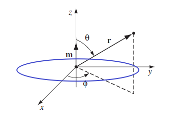 |
Graphical visualization | |
| $\vec{A}$ and $\vec{B}$ when given a dipole | $\vec{A}(\vec{r}) = \frac{\mu_0}{4\pi} \frac{m_0 \sin\theta}{r^2}\hat{e}_\phi$ | if dipole is at origin $\vec{m} = m_0 \hat{e}_z$ |
| $\vec{B}(\vec{r}) = \frac{\mu_0 m_0}{4\pi r^2}(2 \cos \theta \hat{e}\rho + \sin \theta \hat{e}\phi)$ | taking $\nabla \times \vec{A}$ with spherical coordinates | |
 |
Visualizatoin of a “Dipole” | |
| $\vec{A}_{dip}$ of rotating charges | $\vec{A}{dip} = \int d\vec{A}{dip}^{loop}$ | for we know that $d\vec{A}{dip}^{loop}=\frac{\mu_0 a^2}{4r^2}\sin( \theta) dI\hat{e}\phi$ for a loop current |
| basically suming over loops of wires. e.g. works by finding $dI = d\lambda \cdot v$ for $v = R\Omega$ | ||
| once we found $\vec{A}{dip}$ recover $\vec{m}$ with $\vec{A}{dip}(\vec{r}) = \frac{\mu_0}{4\pi} \frac{m_0 \sin\theta}{r^2}\hat{e}_\phi$ | ||
 |
cannot use $\vec{m}=\int I d\vec{A}’$ directly as we obviously don’t have a wire loop |
Cycltron Motion
In the generic case we have both $\vec{E}, \vec{B}$, we have both terms in the lorentz Force.
\[\vec{E} = E \hat{x}\\ \vec{B} = B \hat{z}\]Since we know $\vec{B}$ only acts on $\vec{v}_{\perp}$ to the field itself, we decompose the EoM into velocity perpendicular to $B$ and parallel to $B$:
\[m \frac{d\vec{v}_{\perp}}{dt} = q (E_x + \vec{v}_{\perp}\times \vec{B})\\ m \frac{d\vec{v}_{\parallel}}{dt} = 0\]we notice that $\vec{E} \perp \vec{B}$ in this setup, hence $\vec{v}_{\parallel}$ is unaffected. Then we consider solving in cartesian coordiantes:
\[\frac{d\vec{v}_{\perp}}{dt} = \frac{q}{m} (E_x + \vec{v}_{\perp}\times \vec{B})\to \begin{cases} \dot{v}_x = \frac{q}{m} (E_x + Bv_y)\\ \dot{v}_y = -\frac{q}{m} (Bv_x) \end{cases}\]which is a coupled equation and unsymmetric we can solve by:
-
convert to symmetric equation with $v_y’ = v_y + (E_x/B)$, and $v_x’=v_x$ to get:
\[\dot{v}_x' = \frac{q}{m} ( Bv_y')\\ \dot{v}_y' = -\frac{q}{m} (Bv_x')\]essentially shifted a reference frame as if there is no more electric field. Then obviously the motion is a circular loop in this frame.
-
Solve and found that
\[\ddot{v}_x' = -\frac{q^2B^2}{m^2} v_x'\\ \ddot{v}_y' = -\frac{q^2B^2}{m^2} v_y'\]hence we get $w_c = \vert qB/m\vert$ being the rotating frequency, and solution for $v$s are obviously sines and cosines so we are looping.
Note that the drift velocity we fonud here is a specific case of:
\[\vec{v}_{drift} = \frac{\vec{E}\times \vec{B}}{B^2}\]whenever we have both electric field and magnetic field for a moving charge.
(a good exercise here is to a) solve the motion with initial velocity zero, and b) solve the velocity at the bottom of the curve)
Using Biot-Savart Law for Current
Consider using:
\[\vec{B}(\vec{r}) = \frac{\mu_0 I}{4\pi} \int \frac{d\vec{l}(\vec{r}')\times(\vec{r}-\vec{r}')}{|\vec{r}-\vec{r}'|^3}\]to compute the magnetic field at $\vec{r}=(x,0,0)$ WLOG for this
Then:
-
this only integrates over wire, so $d\vec{l}’ = dz’\, \hat{e}_z$ and $\vec{r}’ = (0,0,z’)$
-
then you basically get
\[\vec{B}(\vec{r}) = \frac{\mu_0 I}{4\pi} \int \frac{dz'\hat{e}_z\times(x\hat{e}_x - z'\hat{e}_z)}{[x^2+ z'^2]^{3/2}}\]and yuo will be done
However, it would be wrong if you considered any of the following combination
- $d\vec{l}’ = dz’\, \hat{e}_z$ and $\vec{r}’ = (x’,y’,z’)$
- $d\vec{l}’ = \delta(x’)\delta(y’)dz’\, \hat{e}_z$ and $\vec{r}’ = (0,0,z’)$, which technically works but is wierd
If you are unsure you can always go back to the generic expressoin with $J$, and then
- taking $\vec{J} = \vec{I}(z’)\delta(x’)\delta(y’)$ in our case, then $\vec{I}dl = Id\vec{l}$
- since that is generic, use $\vec{r}’ = (x’,y’,z’)$
(as an exercise, find $B(z)$ for a loop current with radius $R$)
Field of a Solenoid
Due to symmetry we know we can use Ampere’s loops.
But first we need to show that there is no $B_r, B_\phi$ component. How do we argue this? Consider viewing the setup as
| $B_\phi=0$ | $B_r = 0$ |
|---|---|
 |
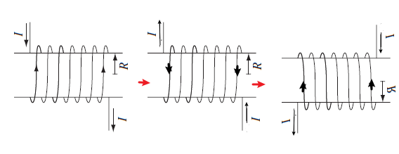 |
where the arguments are simple:
-
for $B_\phi$, such a loop would have $2\pi B_\phi = 0$ using Ampere’s Law
-
for $B_r$, we can suppose there is in the figure image with $B = B\hat{e}_r$
- reverse the current, we would have $-B\hat{e}_r$
- and then flip 180 degrees, still $- B\hat{e}_r$
but the configuration is the same as the first image! Hence $B=0$
Therefore, $B=B_z\hat{e}_z$. So all we need to do is to draw loops that have $z$ component:
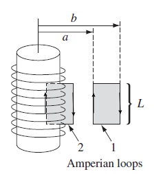
where
- for the second loop we have $B_z(a)L - B_z(b)L = 0$. Hence $B_z(a)=B_z(b)$. But we konw the field is finite so that $B_z(\infty)=0$. Therefore $B_z(r)=0, r>R$
- then for the first lopo we get $B_z(r)L = \mu_0 (nL) I$, hence $B_z(r)=\mu_0 nL$ for $r < R$
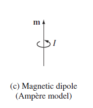
Magnetic Dipole of a Surface
Consider computing $\vec{m}$ of a rotating disk with charge density $\sigma$ and rotation speed $\Omega$:
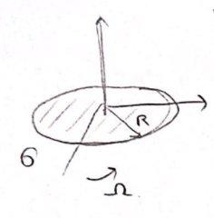
There are two ways to do it:
- consider finding $A$ then match to find $\vec{m}$ (do it as an exercise)
- consider $\vec{m} = \int d\vec{m}^{loop}$
- we know for a loop $d\vec{m}^{loop} = (dI)A = \pi r^2 dI$
- then we also know here that $dI = (d\lambda) v=(\sigma dr)(\Omega r)$
- the integral becomes $\int_0^R \sigma \Omega \pi r^3 dr$
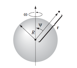
B Field of a rotating shell of charge
Essentially we integrate by summing over loop charges whose $\vec{A}_{dip}$ we already know
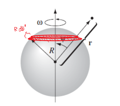
so we consider
\[\vec{A}_{dip} = \int d\vec{A}_{dip}^{loop}\]for which we know in this case the loop wires are the red ones highlighted:
\[d\vec{A}_{dip}^{loop}=\frac{\mu_0 a^2}{4r^2}\sin( \theta) dI\hat{e}_\phi\]and
- $a = R \sin(\theta’)$ in this case
- $dI = (d\lambda )v = (\sigma Rd\theta’)(\Omega R\sin(\theta’))$
- then just put everything together and find $\vec{A}_{dip}$
Finally, we can use
\[\vec{A}_{dip}(\vec{r}) = \frac{\mu_0}{4\pi} \frac{m_0 \sin\theta}{r^2}\hat{e}_\phi\]for $\vec{m} = m_o \hat{e}z$ to easily find $\vec{m}$ of this corresponding $\vec{A}{dip}$
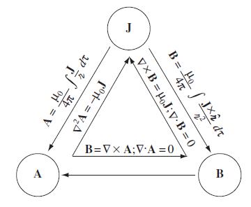
Summary of generic formulas
Chapter 6
Magnetic fields in matter. Basically if we know a material is magnetized with $\vec{M}$ being the dipole per unit volume, what is the field $\vec{B}$ produced by such a magnetization.
- remember that all magnetic effects are due to moving charges
- in a small scale, it can be produced by electrons orbiting = electrons cloud spinning = spinning charged sphere; or it can be electrons self-spin. Both of which basicity create magnetic dipoles and hence $\vec{M}$
| Condition | Equation | Comment |
|---|---|---|
| Paramagnetism due to uniform $\vec{B}$ | $\vec{N} = \vec{m}\times \vec{B}$ | dipole $\vec{m}$ not aligned with external field $\vec{B}$ will cause torque |
| consider electron self-spin as a dipole in this example | ||
| Diamagnetism due to uniform $\vec{B}$ | $\Delta \vec{m}=-\frac{1}{2}e\Delta v R\vec{e}_z = - \frac{e^2R^2}{4m_e}\vec{B}$ | if $\vec{B}=B\hat{e}_z$ is perpendicular to orbit, then it affects centripetal force, hence changing speed |
| $\vec{m}=I\int d\vec{a}=-\frac{1}{2}evR\hat{e}_z$ | without external field, $v$ solved from centripetal force being electrostatic attraction | |
| $\frac{1}{4\pi \epsilon_0}\frac{e^2}{R^2}+ev’B = m_e\frac{v’^2}{R}$ | new speed $v’$ for same radius $R$ (due to quantum effect) | |
| $\Delta \vec{m}=-\frac{1}{2}e\Delta v R\vec{e}_z = - \frac{e^2R^2}{4m_e}\vec{B}$ | opposes the applied field $\vec{B}$ | |
| Torque’s effect of aligning the dipole is little in this case. | ||
| Magnetic Moment $\vec{M}(\vec{r})$ | $\vec{M}(\vec{r})\approx \sum \vec{m}$ | think of $\vec{M}$ as specifying a collection of tiny dipoles $\vec{m}$ |
| $\vec{A}$ from $\vec{M}$ | $\vec{A}=\frac{\mu_0}{4\pi} \sum_{i} \frac{\vec{m}\times \hat{r}}{\vert \vec{r}-\vec{r}_i’\vert }$ | discrete case |
| $\vec{A}=\frac{\mu_0}{4\pi} \int \frac{\vec{m}\times \hat{r}}{\vert \vec{r}-\vec{r}’\vert }d^3r’$ | continuous case | |
| note that $\hat{r}=\vec{r}/\vert \vec{r}\vert$ | ||
| $\vec{A}_{dip} = \frac{\mu_0}{4\pi} \frac{\vec{m}\times \hat{r}}{\vert \vec{r}-\vec{r}’\vert }$ | derived because we know the field of a single dipole | |
| Most generic form of finding $\vec{B}$ from given $\vec{M}$ | ||
| $\vec{A}$ from $\vec{M}$ using bound currents | $\vec{A}=\frac{\mu_0}{4\pi} \int_{all} \frac{\vec{J}_{b}}{\vert \vec{r}-\vec{r}’\vert }d^3r’+\frac{\mu_0}{4\pi}\oint \frac{\vec{K}_b}{\vert \vec{r} - \vec{r}’\vert }dA’$ | mathematically same as above |
| $\vec{J}b \equiv \nabla \times \vec{M},\quad \vec{K}{b} \equiv \vec{M}\times \hat{n}$ | for $\hat{n}$ points from the magnetized material to vacuum | |
| Physical Interpretation of Bound Charges | $\vec{K}_b = \vec{M}\times \hat{n}$ | imagine uniform magnetized material = uniform tiny current loops |
| Hence inner loops cancel, we only have net outer current | ||
| $\vec{J}_b = \nabla \times \vec{M}$ | If non-uniform magnetized material, then net $\vec{J}_b$ comes from difference in current loops | |
| Auxiliary Field $\vec{H}$ | $\vec{H}=\frac{1}{\mu_0}\vec{B}-\vec{M}$ | more useful than $\vec{B}$ when we have magnetized material |
| $\vec{H}$ often in the same direction as $\vec{B}$ and $\vec{M}$ | ||
| The magnetic parallel of $\vec{E}$ field. ($\vec{B}$ would be a parallel to $\vec{D}$ instead) | ||
| $\nabla \times \vec{B} = \mu_0 \vec{J}{total} = \mu_0 (\vec{J}_b + \vec{J}{free})$ | derivation from Ampere’s Law, then use $\vec{J}_b = \nabla \times \vec{M}$ | |
| true in general | ||
| Differential and Integral form of $\vec{H}$ | $\nabla \times \vec{H} = \vec{J}_{free}$ | follows from the above |
| $\oint \vec{H}\cdot d\vec{l} =\int \vec{J}{free} \cdot d\vec{A}=I{free_{enc}}$ | very useful when we have symmetry | |
| Linear Material | $\vec{M} \equiv \chi_m \vec{H}$ | $\vec{J}{free} \to \vec{B}{free}\to \vec{M}$ if material is magnetizable |
| $\vec{B}= \mu_0 (1+ \chi_m)\vec{H}=\mu \vec{H}$ | derived from $\vec{H}=\frac{1}{\mu_0}\vec{B}-\vec{M}$ | |
| $\mu = \mu_r \mu_0 \equiv \mu_0(1 + \chi_m)$ | ||
| Boundary Conditions for $\vec{H}$ | $H^\perp_{above}-H^\perp_{below}=-(M^\perp_{above}-M^\perp_{below})$ | derived from Drawing a box on the surface and using $\oint \vec{H}\cdot d\vec{S}=-\int \vec{M}\cdot d\vec{S}$ (which comes from the definition of $\vec{H}$) |
| $H^\parallel_{above}-H^\parallel_{below}=K^{\perp}_{free}$ | from below | |
| $\vec{H}^\parallel_{above}-\vec{H}^\parallel_{below}=\vec{K}_{free}\times \hat{n}$ | derived from Drawling a loop on the surface and using $\oint \vec{H}\cdot d\vec{l}=I_{free_{enc}}$. In this case we have two directions for $\vec{H}^\parallel$, hence the RHS. | |
| Useful for solving Laplacian with $\vec{H}=-\nabla W$ | ||
| Magnetic Scale Potential $W$ | $\vec{H}=-\nabla W$ | if $\vec{J}_{free}=0$ so that $\nabla \times \vec{H}=\vec{0}$ |
| $\nabla^2 W = \nabla \cdot \vec{M} = 0$ | if $\vec{\nabla}\cdot \vec{M}=0$, then it is Laplacian. True automatically if linear material. | |
| Combine with B.C.to solve Laplacian as in electrostatics | ||
| With very restrictive condition it holds | ||
| Field of Solenoid + Linear Material | $\vec{B}{in}=\mu_r \vec{B}{vac_{in}}$ | putting a linear material inside solenoid further increases the field produced |
| derived easily from drawing Ampere loops and using $\oint \vec{H}\cdot d\vec{l}=I_{free_{enc}}$ |
Calculate $\vec{B}$ from Bound Currents
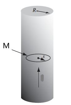
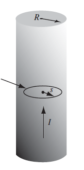
Suppose you are given a material with frozen in magnetization such that $\vec{M}=M\hat{e}_z$ inside the cylinder. The question is what is the magnetic field everywhere.
| Setup | Setup with Bound Currents |
|---|---|
 |
 |
We know we can get $\vec{B}$ either:
- calculate $\vec{A}$ then do $\vec{B}=\nabla \times \vec{A}$. You wil see that we have many ways to find $\vec{A}$
- if finite currents to integrate through, consider treating them as rotating charge = current loops $\vec{A}{dip} = \int d\vec{A}{dip}^{loop}$
- or compute $\vec{A}$ from the bound charges using the generic formula above (a lot of work)
- calculate $\vec{B}$ directly by treating bound currents as currents (faster here)
- calculate using $\vec{H}$ if linear material (not applicable here)
- if $\vec{J}_b=0$ and $\nabla \cdot \vec{M}=0$, then can use $\vec{H}=-\nabla W$ and solve laplacian
We first compute the bound currents and notice that:
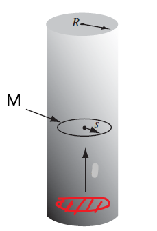
\[\begin{align*} \vec{J}_b &= \nabla \times \vec{M} = \vec{0}\\ \vec{K}_b &= \vec{M}(\vec{r})|_{surf}\times \hat{n} = \begin{cases} 0, & \text{at top/bottom with }\hat{n} = \hat{e}_z\\ M\hat{e}_\phi & \text{at sides with }\hat{n} = \hat{e}_r \end{cases} \end{align*}\]With this we have the graph on the right, for currents going around the cylinder. In this case, we know that $\vec{B}=B_z\hat{e}_z$, which makes the computation straightforward.
Then we can easily compute $\vec{B}$ given this current by drawing ampere loop:
\[\oint \vec{B}\cdot d\vec{l} = \mu_0 I_{enc}\]Knowing that $\vec{B}_{outer}=\vec{0}$ from a solenoid, we have:
\[B_z(r)L - 0 = \mu_0 L K_b = \mu_0LM\]Hence we obtain
\[\vec{B}(\vec{r}) = \begin{cases} \mu_0 M \hat{e}_z, & r < a\\ 0, & r > a \end{cases}\]which makes sense by right hand rule.
Computing $\vec{A}$ given $\vec{M}$
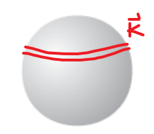
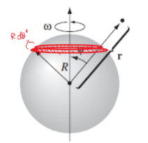
Here we consider some finite bound currents with spherical symmetry, so that we have a spherical shell with given magnetization of $\vec{M}=M\hat{e}_z$:
| Setup | Parallel with Rotating Charges |
|---|---|
 |
 |
First we compute the bound charges, and then decided what to do/which method to take:
\[\begin{align*} \vec{J}_b &= \nabla \times \vec{M} = \vec{0}\\ \vec{K}_b &= \vec{M}(\vec{r})|_{surf}\times \hat{n} = \vec{M}\times \hat{e}_\rho = M\sin \theta \hat{e}_\phi \end{align*}\]So that essentially we have currents on the surface with $M\sin \theta$ dependence. This forbids us to use approaches with Ampere loops, but we realize that this is essentially integrating over many current loops = dipoles:
\[\vec{A}_{dip} = \int d\vec{A}_{dip}^{loop}\]would be usable from previous chapter, which we basically know
\[d\vec{A}_{dip}^{loop}=\frac{\mu_0 a^2}{4r^2}\sin( \theta) dI\hat{e}_\phi\]with $dI = (d\lambda )v = (\sigma Rd\theta’)(\Omega R\sin(\theta’))$. Hence all we need to do is to convert our $K$ to terms in $dI$:
\[\vec{K} = \sigma \vec{v} = \sigma(\Omega R \sin \theta) \hat{e}_\phi = \vec{K}_b = M \sin \theta \hat{e}_\phi\]Then we just basically can find $\vec{A}$, from which we can find $\vec{B}$.
Calculate field using $\vec{H}$ from given $\vec{M}$:
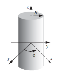
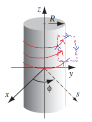
Consider given that $\vec{M} = kr^2 \hat{e}_{\phi}$ inside a cynlinder
| Setup | Ampere Loop |
|---|---|
 |
 |
Then we first know that the field $\vec{B},\vec{H}$ would therefore also be in $\hat{e}_{\phi}$ direction (do not confuse $\vec{M}$ with bound currents here). Hence drawing a Ampere loop inside:
\[\oint \vec{H}\cdot d\vec{l} = 2\pi r H_\phi(r= I_{free_{enc}} = 0\]Hence we easily get $\vec{H}=0$ everywhere. Finally using $\vec{H}=\frac{1}{\mu_0}\vec{B}-\vec{M}$ we get back $\vec{B}$ field by:
\[\vec{B} = \begin{cases} \mu_0 kr^2 \hat{e}_\phi, & r < a\\ 0, & r > a \end{cases}\]since we know $\vec{M}$ as they are given.
- an exercise of this would be to compute using bound currents and arrive at the same solution here.
When to use $\vec{H}$
In general, we can do ampere loops with $\vec{B}$ if we are sure we know all contributions (e.g. from current and from $\vec{M}{induced}$). But consider the case where you have a magnetizable cylinder with some external currents $\vec{J}{free} = I/(\pi R^2)\hat{e}_z$ following through
The finding $\vec{B}$ naively using the loop above would give wrong result:
\[2\pi B_\phi(r) = \mu_0 I \pi \left( \frac{r}{R}\right)^2\]but then yuo have ignored $\vec{M}_{induced}$ which could cause other components in $\vec{B}$. Therefore, the correct way is to consider $\vec{H}$:
\[2\pi H_\phi(r) = I \pi \left( \frac{r}{R}\right)^2\]then using $\vec{H}=\frac{1}{\mu_0}\vec{B}-\vec{M}$ we get $\vec{B}$ (assuming $\vec{M}$ is linear)
Parallels of $\vec{H}$ in Electrostatics:
| Electrostatics | Magnetostatics | |
|---|---|---|
| Linear Material | $\vec{P}=\epsilon_0 \chi_e \vec{E}_{total}$ | $\vec{M} = \chi_m \vec{H}$ |
| Linear Material | $\vec{D} = \epsilon \vec{E}_{total}$ | $\vec{B} = \mu \vec{H}$ |
| Generic | $\vec{D} = \epsilon\vec{E}_{total} + \vec{P}$ | $\vec{B} = \mu_0 (\vec{H}+\vec{M})$ |
so you see that the parallel of $\vec{E}$ is actually $\vec{H}$
Magnetic Scalar Potential $W$
With very restrictive condition a problem can be formulated as a Laplacian. Consider the setup where you have an infinitely long cylinder with $\vec{M}=M\hat{e}_x$. We want to find $\vec{B}$ everywhere.
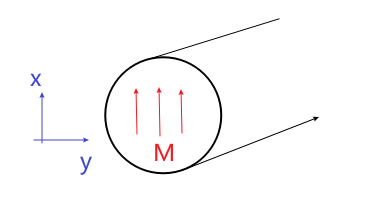
First, it is always a good idea to figure out the bound currents:
\[\begin{align*} \vec{J}_b &= \nabla \times \vec{M} = \vec{0}\\ \vec{K}_b &= \vec{M}(\vec{r})|_{surf}\times \hat{n} = \vec{M}\times \hat{e}_r = M\sin \phi \hat{e}_z \end{align*}\]where we basically converted to cylindrical coordinate $\vec{M}=M(\cos \phi \hat{e}r-\sin \phi \hat{e}\phi)$, and we ignored the top/bottom surface of of the cylinder since it is infinitely long.
Notice that we cannot use Ampere loops here due to $\phi$ dependence, hence we consider Laplacian by realizing that
\[\vec{J}_{free} = \vec{0}\\ \nabla \cdot \vec{M} = \nabla \cdot (M\hat{e}_x)=0\]Therefore Laplacian holds for $\vec{H}=-\nabla W$:
\[\nabla^2 W = 0\]We know the solution for cylindrical Laplacian, but we need boundary conditions:
\[\begin{cases} W_{out}=W_{in},& \text{continuity}\\ H^\perp_{above}-H^\perp_{below}=-(M^\perp_{above}-M^\perp_{below})=M\cos \phi, & \text{B.C.} \\ W_{out}(r \to \infty) = 0\\ |W_{in}(r=0)| \le \infty \end{cases}\]And the solution takes the form of
\[W(r,\phi)=(F_mr^m+G_mr^{-m})[L_m\cos(m\phi)+N_m \sin(m \phi)]\]then solve in the same manner as in electrostatics.