Logistics and Introduction

Discussion/Q&A:

Piazza. Every questions should be sent there.

TA:

Professor: 1 hour before class
Yanda Chen: Tue 6-8pm
Kun Qian: Tue Thur 4:30-5:30pm
Qingyang Wu: Wed 10am-12pm

Grades:

Type	Percentage
Homework *3 (All python)	51%
Midterm *1	15%
Final *1	20%
Tendance	14%
Piazza (extra credit)	3%
Total	103%

Slides:

On the Syllabus
Readings: https://web.stanford.edu/~jurafsky/slp3/

Applications of NLP

Question Answering:

Won the game “Jeopardy” on Feb 16, 2011

Information Extraction

e.g. extraction information from an email, and add the appointment to my calendar

Sentiment/Opinion Analysis

whether if it is a positive review or a negative review

Machine Translation

fully automatic translation between different languages
help human translators to translate text

Current Progress in NLP

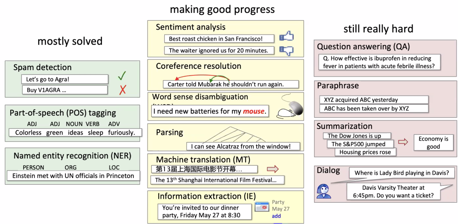
where:

Spam detection would be like a ML binary classification problem
Part-of-Speech (POS): tag every token with their syntactic meaning
Sentiment Analysis: though it sounds like a simply classification problem, we may want to be “context aware” due to sarcasm
Coreference: which person does “he” refers to? (helpful for extracting information)
Parsing: parse the sentence into a tree, e.g. which part is the central piece, which part is purely for description, e.g. understand the functions of different parts of a text. (helpful for summarization)

Difficulties in NLP

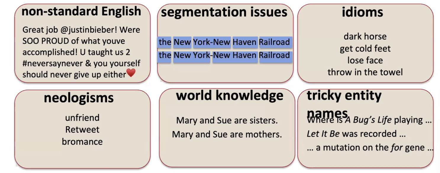
where:

use of Emoji, internet slangs
segmentation of a sentence to break them into parts
idioms: they have deeper/cultural meaning that they superficially mean
tricky entity names: “Let it Be” is the name of a song. “A bug’s life” is name of a show

Overall Syllabus

We will start with theories and statistical NLP
- Viterbi
- N-gram language modeling
- statistical parsing
- Inverted index, tf-id
Programming and Implementations
- using Python

Basic Text Processing

Before almost any natural language processing of a text, the text has to be normalized. At least three tasks are commonly applied as part of any normalization process:

Tokenizing (segmenting) words
Normalizing word formats
Segmenting sentences

Most preprocessing task in NLP involve a set of tasks collectively called text normalization

Normalizing text means converting it to a more convenient, standard form. For example, most of what we are going to do with language relies on first separating out or tokenizing words, lemmatization (e.g. sang, sung, and sings are all form sing), stemming, sentence segmentation, and etc.

Some other nomenclatures:

corpus (plural corpora), a computer-readable corpora collection of text or speech
- e.g. the Brown corpus is a million-word collection of samples from 500 written English texts from different genres
utterance is the spoken correlate of a sentence: “I do uh main- mainly business data processing”
- This utterance has two kinds of disfluencies. The broken-off word main- is fragment called a fragment. Words like uh and um are called fillers or filled pauses.
- Should filled pause we consider these to be words? Again, it depends on the application.

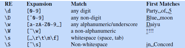
Regular Expressions

Some common usages building regular expressions during preprocessing/extracting some words:

Basics:

Pattern	Matches	Note
`[wW]oodchuck`	Woodchuck, woodchuck	Disjunction `[wW]`
`[1-9]`	any single digit	Ranges: `[1-9]`
`[^A-Z]`	Not an upper case letter	`^` only means negation when used with `[]`
`[^Ss]`, `[^e^]`	Not `S` or `s`, `e` or `^`	e.g. `a^b` means actually matching `a^b`
`a\|b\|c`	same as `[abc]`	More disjunction

Regular expressions with ?/*/+/.

Pattern	Matches	Note
`colou?r`	color, colour	previous character would be optional
`oo*h`		previous charterer would have 0 or more occurrence
`o+h!`		1 or more occurrence
`baa+`
`beg.n`	begin, began, begun

Anchors ^ and $

Pattern	Matches	Note
`^[A-Z]`	Palo	the first character must be `[A-Z]`
`^[^A-Z]`	1Hello	the first character must NOT be `[A-Z]`
`\.$`	Hello.	the last character must be `.`

note that we used escape character as otherwise . means any symbol.

More operators

For Example:

Finding all instance of the word “the” in a given text, assuming the texts are “clean”:

Solution:

Using:

the : misses capitalized The occurrence
[tT]he: also matched other
[^a-zA-Z][tT]he[^a-zA-Z]: works, but would miss the The at the beginning of document
(^|[^a-zA-Z])[tT]he([^a-zA-Z]|$): final version

Note

The process we just went through was based on fixing two kinds of errors

Matching strings that we should not have matched (there, then, other)

False positives (Type I)

accuracy or precision (minimizing false positives)

Not matching things that we should have matched (The)

False negatives (Type II)

Increasing coverage or recall (minimizing false negatives)

Simple Models

We can use Regular Expression as a simple model:

whether if certain words exist in a paragraph -> classify 1 (e.g. if a positive word exist, positive sentiment)
Sophisticated sequences of regular expressions are often the first model for any text processing text

More complicated tasks:

Use regular expression for processing -> use machine learning models

Word Tokenization

Every NLP task needs to do text tokenization:

Tokenization is essentially splitting a phrase, sentence, paragraph, or an entire text document into smaller units, such as individual words or terms. Each of these smaller units are called tokens.

e.g. “New York” and “rock’ n’ roll” are sometimes treated as large words despite the fact that they contain spaces

punctuation will be included/treated as a separate token from words

Some problems that makes this task invovled:

dealing with URLs
dealing with numbers such as $555,500.0$, where punctuations are involved
converting words such as “what’re” to “what are”
depending on application, tokenize “New York” to a single word

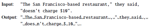
In practice, tokenization runs before any other processing, and needs to be fast. For example, converting:

therefore:

often implemented using deterministic algorithms based on regular expressions compiled into very efficient finite state automata.

programming example:

>>> text = 'That U.S.A. poster-print costs $12.40...'
>>> pattern = r'''(?x) # set flag to allow verbose regexps
... ([A-Z]\.)+ # abbreviations, e.g. U.S.A.
... | \w+(-\w+)* # words with optional internal hyphens
... | \$?\d+(\.\d+)?%? # currency and percentages, e.g.$12.40, 82%
... | \.\.\. # ellipsis
... | [][.,;"'?():-_`] # these are separate tokens; includes ], [
... '''
>>> nltk.regexp_tokenize(text, pattern)
['That', 'U.S.A.', 'poster-print', 'costs', '$12.40', '...']

Another common task is to compute the length of a sentence. While this sounds as just counting the tokenization, depending on application, you might need to think of whether if you should count on lemma or wordform:

\[\text{Seuss's \textbf{cat} in the hat is different from other \textbf{cats}!}\]

so here notice that:

A lemma is a set of lexical forms having the same stem, the same major part-of-speech, and the same word sense
- both $\text{cat}, \text{cats}$ would be count as only 1
A word form is the full inflected or derived form of the word
- $\text{cat}, \text{cats}$ would count as 2 word forms
i.e. how many “lemma” vs “wordform”

Types and Tokens

\[\text{They picnicked by the pool, then lay back on the grass and looked at the stars.}\]

for instance:

Types are the number of distinct words in a corpus; if the set of words in the vocabulary is $V$, the number of types is the word token vocabulary size $\vert V\vert$.
- When we speak about the number of words in the language, we are generally referring to word types.
Tokens are the total number $N$ of running words.
- If we ignore punctuation, the above Brown sentence has 16 tokens and 14 types:
- each type may be exemplified by multiple tokens

Issues

Other than some common issues/choices you need to make in tokenization, such as:

whether or not you should expand what're to what are
should we remove - from Hewlett-Packard?
what should we do with PhD.? Should we treat it as the full acronym?

Other difficulties arises as well:

Issues in Languages.

For instance in German, the word:
\[\text{Lebensversicherungsgesellschaftsangesteller} \to \text{life insurance company employee}\]
is basically four words in one:
- this single word contains four things, so we need to use compound splitter to split into four
In Chinese, the sentence $\text{姚明进入总决赛}$ can be split into:

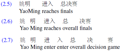
because there is no space! How do we split them into tokens?
- implemented using Greedy search (Maximum Marching), until they cannot be split further
  - this works if you have a dictionary already
- therefore, word tokenization is also called word segmentation since there are no spaces in Chinese

For Example: Maximum Marching

it turns out that it worked pretty well in most of the cases. For illustration purposes, we demonstrate them in English:

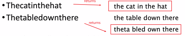
note that in languages such as Chinese they actually work pretty well

but in general, modern probabilistic segmentation algorithms perform even better (baseline: Maximum Matching)

Byte-Pair Encoding for Tokenization

Another popular way of tokenization is to use the data/corpus to automatically tell us what tokens should be. NLP algorithms often learn some facts about language from one corpus (a training corpus) and then use these facts to make decisions about a separate test corpus and its language.

however, a problem is, say we had words such as $\text{low}, \text{new}, \text{newer}$, but see $\text{lower}$ in the test corpus. What should we do?

To deal with this unknown word problem, modern tokenizers often automatically induce sets of tokens that include tokens smaller than words, called subwords.

Subwords can be arbitrary substrings, or they can be meaning-bearing units like the morphemes, e.g. $\text{-est, -er}$
- A morpheme is the smallest meaning-bearing unit of a language; for example the word unlikeliest has the morphemes un-, likely, and -est.
e.g. induce $\text{lower}$ from $\text{low}, \text{-er}$

In general, this is done in two steps:

a token learner: takes a raw training corpus (sometimes roughly pre-separated into words, for example by whitespace) and induces a vocabulary of tokens that will be used
a token segmenter, takes a raw test sentence and segments it into the tokens using the vocabulary

Three algorithms are widely used:

byte-pair encoding (Sennrich et al., 2016),
unigram language modeling (Kudo, 2018),
WordPiece (Schuster and Nakajima, 2012);

there is also a SentencePiece library that includes implementations of the first two of the three

Normalization, Lemmatization, and Stemming

Word normalization is the task of putting words/tokens in a standard format, choosing a single normal form for words with multiple forms, i.e. implicitly define equivalence classes of terms

e.g. ‘USA’ and ‘US’ or ‘uh-huh’ and ‘uhhuh’, so that searching for “USA” should match result with “US” as well

therefore, useful for Information Retrieval: indexed text & query terms must have same form.

more e.g.

Enter: window Search: window, windows

Enter: windows Search: Windows, windows, window

Case Folding

One easy kind of normalization would be case folding: Mapping everything to lower case means that $\text{Woodchuck}$ and $\text{woodchuck}$ are represented identically/same form.

\[\text{SAIL} \iff \text{sail}\] \[\text{US} \iff \text{us}\]

for different applications, we need to think about whether if this is appropriate

helpful for generalization in many tasks, such as information retrieval and speech recognition (uses tend to use lower case more often)
For sentiment analysis and other text classification tasks, information extraction, and machine translation, by contrast, case can be quite helpful and case folding is generally not done.

Lemmatization

Lemmatization: task of determining that two words have the same root, despite their surface differences

e.g. the words sang, sung, and sings are forms of the verb sing.

a lemmatizer maps from all of these to sing.

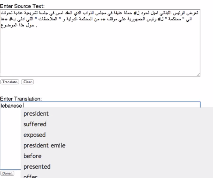
For morphologically complex languages like Arabic, we often need to deal with lemmatization

An example when this is useful would be: in web search, someone may type the string “woodchucks” but a useful system might want to also return pages that mention “woodchuck” with no “s”.

i.e. words with same lemma should be considered as the “same”/a match

More examples include:

\[\{\text{car, cars, car's, cars'}\} \to \text{car}\] \[\text{He is reading detective stories} \to \text{He be read detective story}\]

where:

another helpful case for this would be doing Machine Translation (MT)
how is this done? The most sophisticated methods for lemmatization involve complete morphological parsing of the word.

Morphology is the study of morpheme the way words are built up from smaller meaning-bearing units called morphemes.

Two broad classes of morphemes can be distinguished:

stems — the central morpheme of the word, supplying the main meaning

affix — adding “additional” meanings of various kinds.

For example, the word $\text{fox}$ consists of one morpheme (the morpheme fox) and the word $\text{cats}$ consists of two: the morpheme $\text{cat}$ and the morpheme $\text{-s}$.

Stemming

Lemmatization algorithms can be complex. For this reason we sometimes make use of a simpler but cruder method, which mainly consists of chopping off word-final stemming affixes. This naive version of morphological analysis is called stemming.

Stemming refers to a simpler version of lemmatization in which we mainly just strip suffixes from the end of the word

For instance:

\[\text{automate, automatic, automation} \iff \text{automat}\]

And for paragraphs:

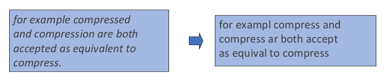
sometimes Stemming is not very useful

often used in information retrieval to condense/compress information
one popular algorithm would be the Porter’s Algorithm

Porter’s Algorithm

In short, The algorithm is based on series of rewrite rules run in series, as a cascade, in which the output of each pass is fed as input to the next pass:

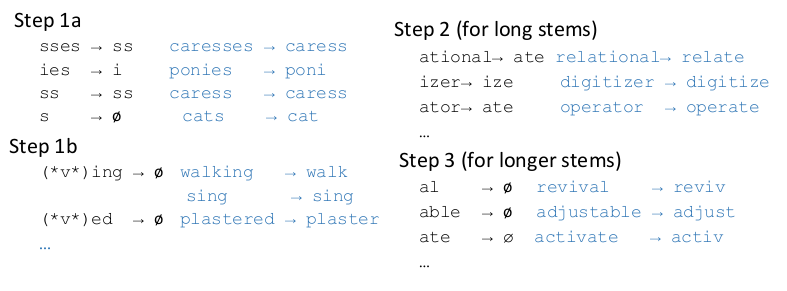
where:

step 1b: removes ing/ed
again, works pretty well for simple texts

Sentence Segmentation

Another important step in preprocessing (related to tokenization) would be separating into sentences. The most useful cues for segmenting a text into sentences are punctuation, like periods, question marks, and exclamation points. However:

Question marks and exclamation points are relatively unambiguous markers of sentence boundaries
Periods, on the other hand, are more ambiguous.
- e.g. abbreviations such as Mr. or Inc., numbers such as $4.3$

In general, it can be solved using machine learning models or hand-written rules:

Rule-based: Stanford CoreNLP toolkit (Manning et al., 2014),
- for example sentence splitting is rule-based, a deterministic consequence of tokenization
- hand-written rules basically hard-coded rules (if/elif/...) or related to regular expressions
Machine Learning: decision tree models
1. Looks at a “.”
2. Decides EndOfSentence/NotEndOfSentence
3. Classifiers: hand-written rules, regular expressions, or machine-learning

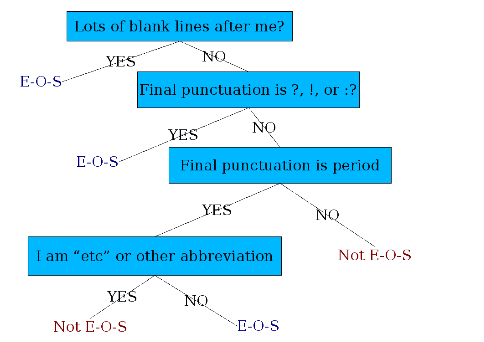
For Example: Machine Learning model for Sentence Segmentation

Often we just use a decision tree for this

Construct features:

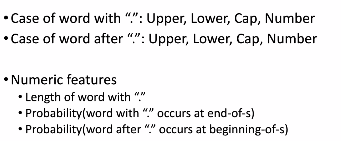
how to choose good features is the key part.
Run the Decision Tree. Output could look like:

Or, we can use other classifiers such as Logistic Regression, SVM, NN, etc.

Minimum Edit Distance

Much of natural language processing is concerned with measuring how similar two strings are.

e.g. popping up autocompletion

Edit distance gives us a way to quantify both of these intuitions about string similarity.

e.g. $\text{graffe}$ with $\text{giraffe}$

Minimum edit distance between two strings is defined as the minimum number of (weighted) editing operations (operations like insertion, deletion, substitution) needed to transform one string into another.

e.g. $\text{graffe}$ to $\text{giraffe}$ would require one

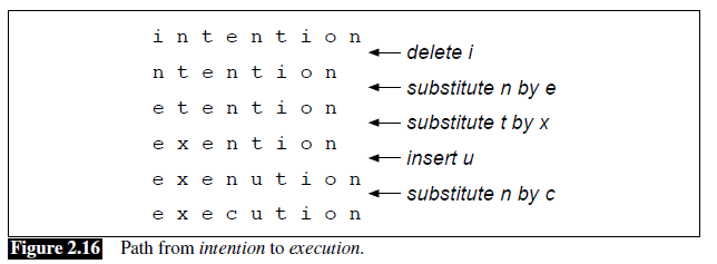
e.g. $\text{intention}$ and $\text{execution}$, for example, is $5$ (without weighting)

(delete an $i$, substitute $e$ for $n$, substitute $x$ for $t$, insert $c$, substitute $u$ for $n$)

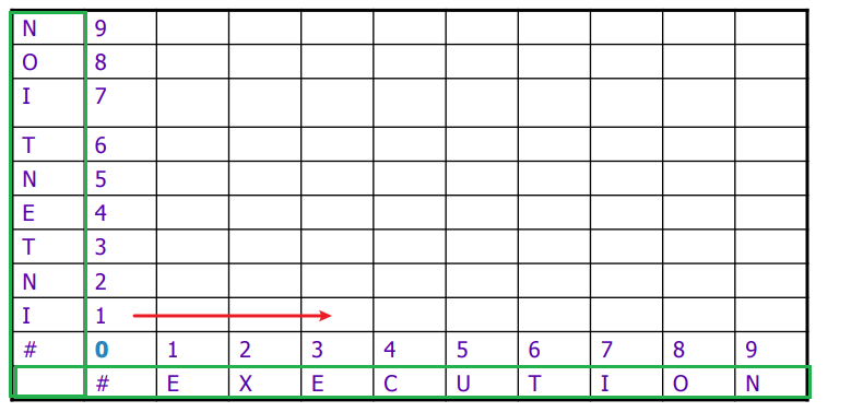
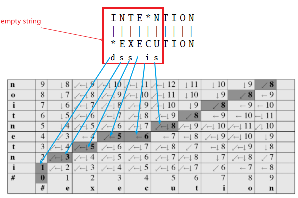
But the problem is, how do we algorithmically do it. First, we may want to visualize the result:

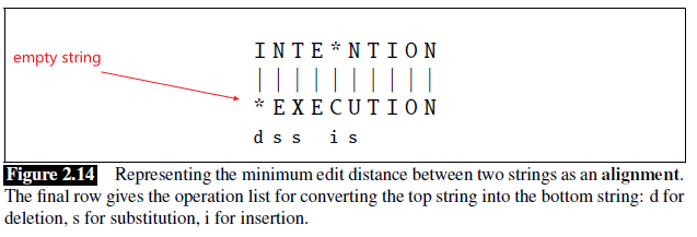
here we are:

given an alignment: a correspondence between substrings of the two sequences.
- $I$ aligns with the empty string, $N$ with $E$, and so on
below the aligned string is operation list for converting the top string into the bottom string: $d$ for deletion, $s$ for substitution, $i$ for insertion
therefore, the minimum edit distance is $5$ because this is already the best alignment

Additionally:

We can also assign a particular cost or weight to each of these operations. The Levenshtein distance between two sequences is the simplest weighting factor in which each of the three operations has a cost of $1$
An alternative version of his metric in which each insertion or deletion has a cost of $1$ and substitutions are not allowed.
- This is equivalent to allowing substitution, but giving each substitution a cost of $2$ since any substitution can be represented by one insertion and one deletion

Minimum Edit Distance Algorithm

Intuition

Our final aim is to produce something like this

Imagine some string (perhaps it is $\text{exention}$) that is in this optimal path (whatever it is).

if $\text{exention}$ is in the optimal operation list, then the optimal sequence must also include the optimal path from $\text{intention }$ to $\text{exention}$.

all the other path we can forget

Then, iteratively compute it:

from $\text{intention}$ to $\text{*}$ (empty string, base case)

from $\text{intention}$ to $\text{e}$

from $\text{intention}$ to $\text{ex}$

from $\text{intention}$ to $\text{exe}$

etc

from $\text{intention}$ to $\text{execution}$

In reality since you can also start from $\text{execution}$, it would be a 2D matrix

Basically this is solved by dynamic programming, which are solutions that apply a table-driven method to solve problems by combining solutions to sub-problems

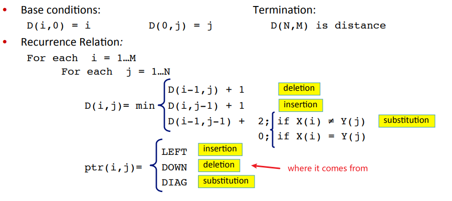
Before showing the main algorithm, we use the notation that:

$*$ is an empty string
$X,Y$ are inputs of length $n,m$
$X[1..i],Y[1..j]$ are the first $i$ characters of $X$, and first $j$ characters of $Y$
we will be filling up a matrix, call it $D$. Our result is basically $D[n,m]$

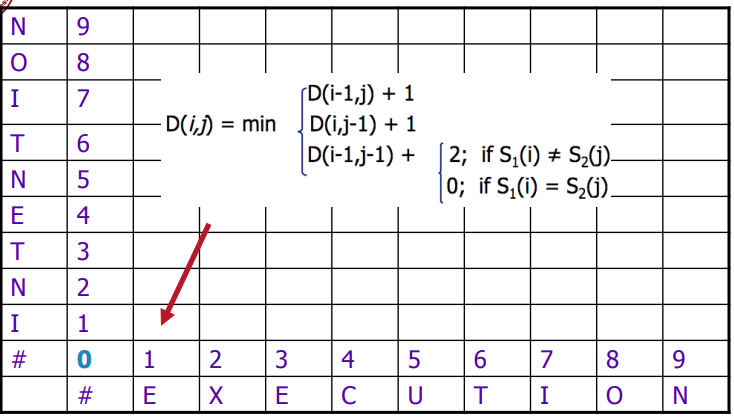
Then, the update rule is simply

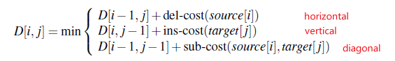
i.e. choosing the best path given the previous bests, which are $D[i-1,j], D[i,j-1], D[i-1,j-1]$.

we used $\text{sub-cost}$ for substitution cost so that user can specify the weights.
here, we will use $\text{sub-cost}=2$, $\text{del-cost}=\text{ins-cost}=1$

Therefore, the algorithm is:

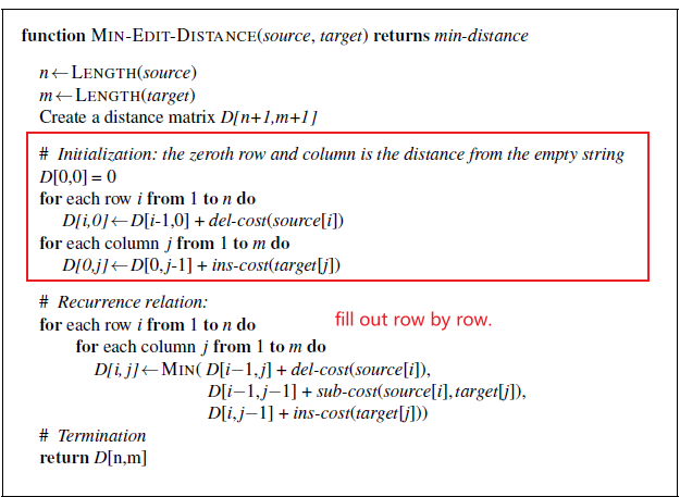
Therefore, it can be easily seen that:

Space Complexity: $O(nm)$
Time complexity: $O(nm)$

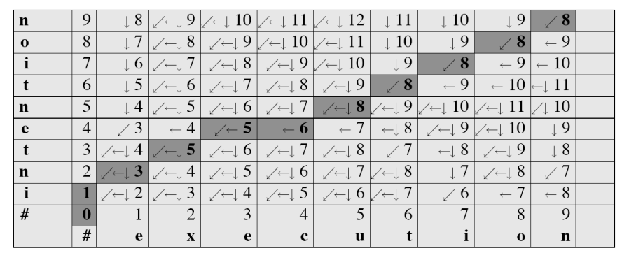
For Example:

First we initialize
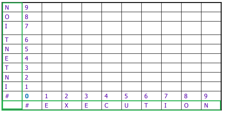
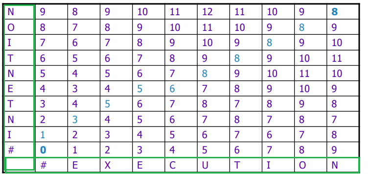
Then, we fill it up row by row

which works since for each computation, the 3 inputs $D[i-1,j], D[i,j-1], D[i-1,j-1]$ would have already been computed.
- we could also go column by column, from bottom up
fill up and return the top right

Note that, the optimal path at each stage is outlined here (done by backtracking)

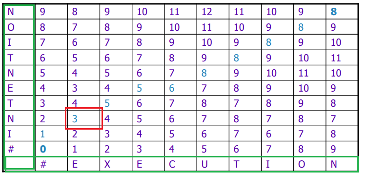
The value $3$ here would mean the minimal cost to go from $\text{IN}$ to $\text{E}$. We can follow the path:

cost $0$ from start
cost $1$ to go from $I \to *$
- delete $I$
cost $3$ to go from $\text{IN} \to \text{E}$
- replace $N \to E$

Alignment

Recall that an alignment basically is the optimal path for edit distance:

Therefore, since it is just the optimal path, we only need to store, for each $D[i,j]$. where did the best previous path come from:

since technically a cell $D[i,j]$ could be optimally reached from several path, the result is NOT unique

for programming, we usually just pick the first in the list
when done, to perform the backtrace, i.e. draw the optimal path from the table, we need $O(n+m)$

The graphical result looks like:

For Example:

Consider how this part comes about from our optimal path

Language Models

The task we are considering is predicting the next few words someone is going to say? What word, for example, is likely to follow

\[\text{Please turn your homework ...}\]

In the following sections we will formalize this intuition by introducing models that assign a probability to each possible next word. The same models will also serve to assign a probability to an entire sentence. So that:

\[P(\text{all of a sudden I notice three guys}) > P(\text{guys all I of notice three a sudden})\]

This would be useful in:

identify words in noisy, ambiguous input, like speech recognition.
For writing tools like spelling correction or grammatical error correction
- $\text{Their are two midterms}$, in which $\text{There}$ was mistyped as $\text{Their}$
Assigning probabilities to sequences of words (sentences) is also essential in machine translation.

Models that assign probabilities to sequences of words are called language model, or LMs.

In this chapter we introduce the simplest model that assigns probabilties to sentences and sequences of words, the n-gram.

An n-gram is a sequence of $n$ words:

a $2$-gram (which we’ll call bigram) is a two-word sequence of words like $\text{please turn}$, or $\text{turn your}$

a 3-gram (a trigram) is a three-word sequence of words like $\text{please turn your}$, or $\text{turn your homework}$.

We will see how n-gram models to estimate the probability of the last word of an n-gram given the previous words, and also to assign probabilities to entire sequences.

N-Grams

Essentially, we would be interested in computing:

\[P(W_1, W_2, ..., W_n)\]

for assigning probability to a given sequence of words.

note that this is a joint probability, which means order matters. e,g. $P(X_1 = 1,X_2 =0) \neq P(X_1=0,X_2=1)$

For predicting next word:

\[P(W_5| W_1, W_2, ..., W_4)\]

Language model, again, needs to be able to compute those probabilities.

The question is how? If we naively want to estimate:

\[P(X_1, ...,X_n) \approx \frac{\text{Count}(X_1,...X_n)}{\text{All Sentences}}\]

The problem is that combination of $X_1,…,X_n$ might not even be there for $n$ being large.

doesn’t appear in training set (usually just a large corpus) doesn’t mean chance of occurring is $0$
need Laplace Smoothing, as you shall see soon

We know that a joint:

\[\begin{align*} P(X_1,...,X_n) &= P(X_1)P(X_2|X_1)P(X_3|X_1,X_2)...P(X_n|X_1,...X_{n-1})\\ &= P(X_1)P(X_2|X_{1})P(X_3|X_{1:2})...P(X_n|X_{1:n-1})\\ &= \prod_{i=1}^nP(X_i|X_{1:i-1}) \end{align*}\]

But still, we are left we computing for $i = n$, or any large $i$:

\[P(X_i|X_1, ..., X_{k-1})= \frac{P(X_1,...,X_{k-1},X_k)}{P(X_1,...X_{k-1})}\]

using law of total probability. Therefore:

\[P(X_i|X_1, ..., X_{k-1}) \approx \frac{\text{Count}(X_1,...,X_{k-1},X_k)}{\text{Count}(X_1,...X_{k-1})}\]

So the same problem persist.

Yet we can approximate this using Markov’s Assumption

Markov models are the class of probabilistic models that assume we can predict the probability of some future unit without looking too far into the past.

thus the n-gram (which looks $n-1$ words into the past only)

e.g. $n=2$ means we only consider up to $1$ word in the past, i.e. only $P(X_i\vert X_{i-1})$

so that:
\[P(\text{the}|\text{its water is so transparent that})\to P(\text{the}|\text{that})\]

Therefore, the n-gram model basically says:

\[\begin{align*} P(X_1,...,X_m) &= \prod_{i=1}^m P(X_i|X_{i-n+1}, ..., X_{i-1}) \end{align*}\]

Then to formally find out estimates for each $P(X_i\vert X_{i-n}, …, X_{i-1})$, we consider them as parameters and perform a MLE.

in a bigram case, where $n=2$, each parameter $P(X_i\vert X_{i-1})$ can be estimated using MLE to yield:
\[P_{MLE}(X_i | X_{i-1}) = \frac{\text{Count}(X_{i-1},X_{i})}{\text{Count}(X_i)}\]
notice that the demotivator is a unigram probability
In general:
\[P_{MLE}(X_i | X_{i-n+1:i-1}) = \frac{\text{Count}(X_{i-n+1:i-1},X_{i})}{\text{Count}(X_{i-n+1:i-1})}\]

For Example

Consider our corpus being given as three sentences, the start is measured by <s> and end </s>

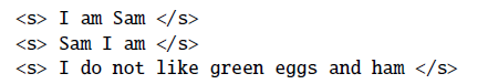
Suppose we are using bigram. Then we can compute some of the bigrams being

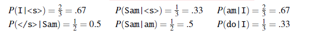
For Example:

Consider using bigram, and recall that:

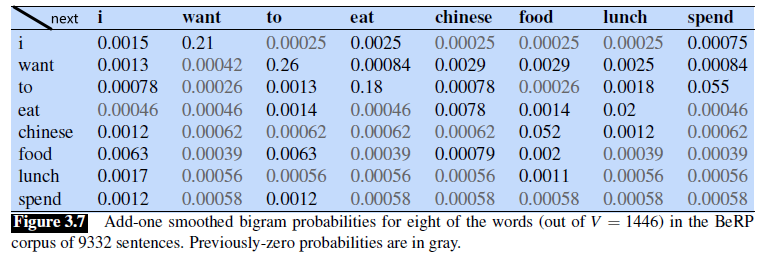
\[P_{MLE}(w_i | w_{i-1}) = \frac{\text{Count}(w_{i-1},w_{i})}{\text{Count}(w_i)}= \frac{\text{Count}(w_{i-1},w_{i})}{\sum \text{Count}(w_i,w_{i-1})}\]

Let the unigram probabilities be given:

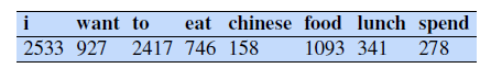
And the bigram counts have been filled

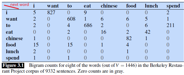
Then we can compute the probability of a sentence

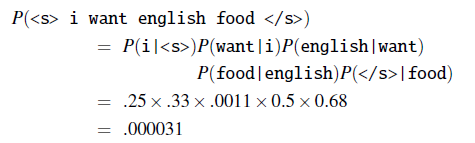
Some practical issues

in practice to generate sentences that makes sense, it is more often to use trigram or 4-gram, depending on how much data you have for training
We always represent and compute language model probabilities in log probability, e.g. instead of $0.000031$, we use $\log (0.000031)$.
- This is because probabilities are (by definition) less than or equal to $1$, the more probabilities we multiply together, the smaller the product becomes. Multiplying enough n-grams together would result in numerical underflow
- $\log$ is good since it is monotonously increasing anyway
- this could also speed up computation, because we can convert our probability output
  \[\log (p_1 \times p_2 \times ... \times p_n) = \log(p_1) + \log(p_2) + ... + \log(p_n)\]
  becomes addition

Evaluating Language Models

In general there are two ways to evaluate:

an intrinsic evaluation of a language model we need a test set
- so measures the quality of a model independent of any application
an extrinsic evaluation: evaluate the performance of a language model by to embedding it in an application and measure how much the application improves
- the “real metric”, but far too expensive
- e.g. put into auto-corrector, and compare how many misspelled words corrected properly

Perplexity

In practice we don’t use raw probability as our metric for evaluating language model, but a variant called perplexity

Perplexity

Consider a word sequence/sentence of $W_1, …, W_n$
\[PP(W_1, W_2, ..., W_n) \equiv PP(W)\]
Then:
\[\begin{align*} PP(W) &= P(W_1,W_2, ..., W_n)^{-1/n}\\ &= \sqrt[n]{\frac{1}{P(W_1,W_2, ..., W_n)}}\\ &= \sqrt[n]{\frac{1}{\prod_{i=1}^nP(W_i|W_{1:i-1})}} \end{align*}\]
is the exact definition.

The intuition of what perplexity measures is as follows:

in fact:
\[\text{perplexity} = 2^{\text{entropy}}\]
where:
- $\text{entropy}$ is the average number of bits that we need to encode the information
- so $\exp$ of the entropy is the total amount of all possible information
hence, instead of just computing the probability, consider a measure of the “average of choices per word”. The higher it is, the more “choices” you have, then the more random is your language model.
therefore, minimizing perplexity is equivalent to maximizing the test set probability according to the language model

Note

In practice, since this sequence $W$ will cross many sentence boundaries, we need to include the begin- and end-sentence markers <s> and </s> in the probability computation.

We also need to include the end-of-sentence marker </s> (but not the beginning-of-sentence marker <s>) in the total count of word tokens $N$.

if you think about perplexity as the “average of choices per word”, then it makes sense that we do not consider <s> since it must have always started with that

For Example

If we use a Bigram model:

\[PP(W)= \sqrt[n]{\frac{1}{\prod_{i=1}^nP(W_i|W_{i-1})}}\]

For Example: Computing Perplexity

Consider two models that have trained on digits, i.e. $0\sim 9$ and know that:

$P(W_i)=1/10$ is constant
$P(W_i)=1/90$ but $P(W=0)=9/10$

Then if we see a text with $N$ words that look like:

\[\text{0 0 0 3 0 0 3 0 ....}\]

then:

the perplexity of the first model:

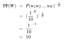
where we are ignoring the start <s> and end </s> for now
the perplexity of the second model is lower since it modelled that on average, the choice of next of next word being $0$ is high.

We trained unigram, bigram, and trigram grammars on 38 million words (including start-of-sentence tokens) from the Wall Street Journal, using a 19,979 word vocabulary. We then computed the perplexity of each of these models on a test set of 1.5 million words.

The table below shows the perplexity of a 1.5 million word WSJ test set according to each of these grammars

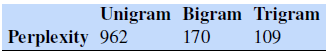
so basically Trigram is doing the best here.

Sampling Sentence from LM

One important way to visualize what kind of knowledge a language model embodies is to sample from it.

Sampling from a distribution means to choose random points according to their likelihood
since our distribution basically are $P(w_i\vert w_{i-k+1:i-1})$, we treat this as a distribution and randomly sample from it

For example, suppose we have a Bigram Model. Using Shannon Visualization Method:

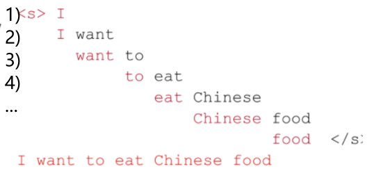
where:

consider $P(w\vert \text{})$ as a distribution for all token $w$. **Randomly sample from it**
- in this case, we got $\text{I}$
consider $P(w\vert \text{ I})$ as a distribututoin for all token $w$. Randomly sample from it
- in this case, we got $\text{want}$
continues until we sampled $\text{</s>}$

Notice that we did not simply pick the most probable ones. Because in the end we will be more likely to generate sentences that the model thinks have a high probability and less likely to generate sentences that the model thinks have a low probability.

Other Examples

Then, if we you this idea to generate texts from Shakespeare (by training on Shakespeare corpus)

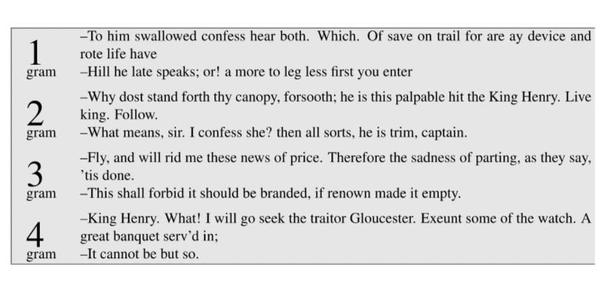
where the output is almost garbage. This is because:

we are using a vocab of $V=29066$ unique tokens, with a corpus of total size $884647$ tokens.
Even Shakespeare only produced around $300,000$ bigrams from the all possible $V^2 = 844 * 10^6$ bigrams. This means that $99.96\%$ of the possible bigrams were never seen in the training corpus (have zero entries in the table)
- so if it happens that one of the bigrams appeared in test corpus, we obvious won’t be able to get that.

So, one big problem for simple language models is their ability to generalize to unseen texts.

On the other hand, if the test and training corpus are somewhat similar:

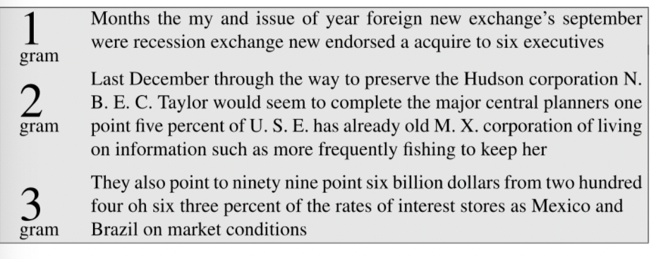
then it seems to work.

this is based on wall street journal corpus

Generalization and Zeros

The n-gram model, like many statistical models, has performance dependent on the training corpus.

This brings the following problems of LM:

One implication of this is that the probabilities often encode specific facts about a given training corpus.
- e.g. if the corpus is about food, then most of the vocabs/structures will be steered towards that
Another implication is that $n$-grams do a better and better job of modeling the training corpus as we increase the value of $N$.
- i.e. higher order $N$-gram models tends to perform better
- however, this then requires a larger training corpus or a larger storage for the probability matrix, which could go $O(V^N)$ for a corpus with $V$ vocab and $N$-gram is used.
  - though this can be optimized as we are having a sparse matrix
Models are often subject to the problem of sparsity. Because any corpus is limited, some perfectly acceptable English word sequences are bound to be missing from it.
- i.e. phrases in test dataset is never seen in train dataset. Then obviously this won’t work
- in real life, this happens

For example: Sparsity

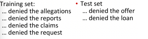
Then:

\[P( \text{offer} | \text{ denied the}) = 0\]

since it was never seen in.

this happens very often in real life applications
notice that this problem we assumed that we have seen all words, but haven’t seen the specific phrase (i.e. this specific combination). Another different problem is that you might not have seen the word!

Note

These zeros have two very serious consequences:

First, their presence means we are underestimating the probability of all sorts of words that might occur, which will hurt the performance of any application we want to run on this data.

Second, if the probability of any word in the test set is 0, the entire probability of the test set is 0.

By definition, perplexity is based on the inverse probability of the test set. Thus if some words have zero probability, we can’t compute perplexity at all, since we can’t divide by 0!

Unknown Words

Before, we showed a problem we assumed that we have seen all words, but haven’t seen the specific phrase (i.e. this specific combination). Another different problem is that you might not have seen the word!

In a closed vocabulary system the test set can vocabulary only contain words from this lexicon, and there will be no unknown words

An open vocabulary system vocabulary is one in which we model these potential unknown words in the test set by adding a pseudo-word called <UNK>.

The percentage of OOV (out of vocabulary) open words that appear in the test set is called the OOV rate.

There are two common ways to train the probabilities of the unknown word model <UNK>.

The first one is to turn the problem back into a closed vocabulary one by choosing a fixed vocabulary in advance:
1. Choose a vocabulary (word list) that is fixed in advance (without looking at the training set)
2. Convert in the training set any word that is not in this set (any OOV word) to the unknown word token <UNK> in a text normalization step.
3. Estimate the probabilities for `` from its counts</mark> just like any other regular word in the training set.
Second alternative, in situations where we don’t have a prior vocabulary in advance, is to create such a vocabulary implicitly
1. replace words in the training data by <UNK> based on their frequency (i.e. threshold it).
  - e.g. replace by <UNK> all words that occur fewer than $n$ times in the training set
2. proceed to train the language model as before, treating <UNK> like a regular word.

Then, when testing our model, we use the probability with <UNK> when seeing an unknown word.

i.e. use that when computing probability of seeing a text/perplexity

However, The exact choice of <UNK> model does have an effect on metrics like perplexity.

A language model can achieve low perplexity by choosing a small vocabulary and assigning the unknown word a high probability.
For this reason, perplexities should only be compared across language models with the same vocabularies

Smoothing

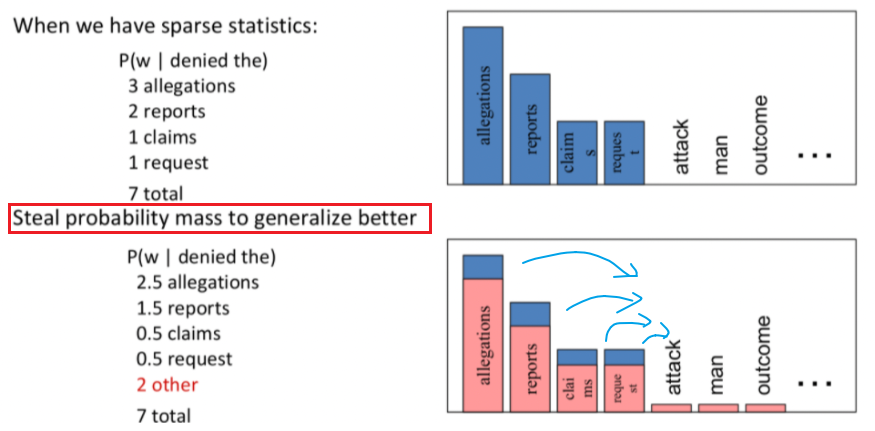
Now, we go back to the problem that vocabs are seen, but the specific phrase/combination are not seen.

Intuition

To keep a language model from assigning zero probability to these unseen events, we’ll have to shift a bit of probability mass from some more frequent events and give it to the events we’ve never seen.

This modification is called smoothing or discounting

So for instance:

In general, there are many ways to do smoothing:

Laplace (add-one) smoothing,
add-k smoothing
interpolation
stupid backoff
Kneser-Ney smoothing

Laplace Smoothing

In reality, one simple way is to use Laplace Smoothing

Laplace Smoothing: add one to all the n-gram counts, before we normalize them into probabilities..

does not perform well enough to be used smoothing in modern $n$-gram models

but it usefully introduces many of the concepts that we see in other smoothing algorithms, gives a useful baseline

Let us first recall that our MLE estimate without smoothing was like (for Bigram)

\[P_{MLE}(w_i | w_{i-1}) = \frac{\text{Count}(w_{i-1},w_{i})}{\text{Count}(w_i)}= \frac{\text{Count}(w_{i-1},w_{i})}{\sum \text{Count}(w_i,w_{i-1})}\]

we needed $\sum \text{Count}(w_i,w_{i-1})$ because it is $\text{Count}(w_i,w_{i-1})$, i.e. the element in our bigram frequency matrix that gets added 1.

also notice that we don’t need gradient descent type algorithm, as this is a probabilistic model

Therefore, the Add-1 estimate is simply:

\[P_{Laplace}(w_i | w_{i-1}) = \frac{\text{Count}(w_{i-1},w_{i}) + 1}{\sum( \text{Count}(w_{i-1},w_{i}) + 1)}=\frac{\text{Count}(w_{i-1},w_{i}) + 1}{\text{Count}(w_{i-1}) + V}\]

where notice that:

$V$ is the size of vocabulary, which makes sense since $P$ needs to add up to 1

For Example:

When added smoothing the bigram frequency matrix looks like

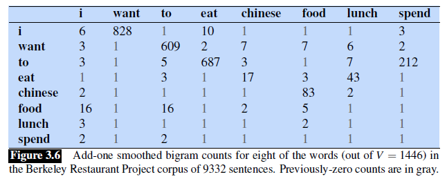
where:

many of the $1$ entries were $0$ before hand.
Basically all entries are added $1$ to it

Now we can compute the conditional probability

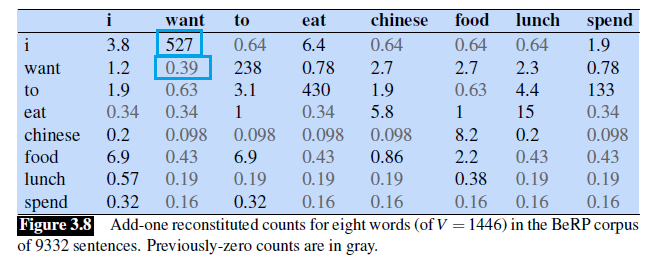
To see the smoothing effect more easily, we can reconstruct the count/frequency matrix by treating:

\[P_{ \text{Laplace}}(w_n | w_{n-1}) \equiv \frac{ \text{Count}^*(w_{n-1}w_n)}{\text{Count}(w_{n-1})} = \frac{\text{Count}(w_{i-1},w_{i}) + 1}{\text{Count}(w_{i-1}) + V}\]

Then we can easily get:

\[\text{Count}^*(w_{n-1}w_n) =\frac{(\text{Count}(w_{i-1},w_{i}) + 1 ) * \text{Count}(w_{n-1})}{\text{Count}(w_{i-1}) + V}\]

This means that the frequency becomes:

Note

In reality:

add-1 isn’t used for N-grams. We’ll see better methods

But add-1 is used to smooth other NLP models

e.g. for text classification, or other domains where the number of zeros isn’t so huge.

Add-k Smoothing

Why add-1? Sometimes you may want to shift a bit less of the probability to unseen events, so that you might pick $k=0.5$, or $k=0.05$ for instance to:

\[P_{Laplace}(w_i | w_{i-1}) = \frac{\text{Count}(w_{i-1},w_{i}) + k}{\sum( \text{Count}(w_{i-1},w_{i}) + k)}=\frac{\text{Count}(w_{i-1},w_{i}) + k}{\text{Count}(w_{i-1}) + kV}\]

where:

now we may want to know what $k$ is the most optimal. This can be done, for example, by optimizing on a devset.

Backoff and Interpolation

Again, recall that the problem is no examples of a particular trigram (for example), $w_{n-2}w_{n-1}w_{n}$ is seen such that:

\[P(w_n|w_{n-2}w_{n-1}) = 0\]

However, we can maybe just rely on/estimate its probability by using the bigram probability $P(w_n \vert w_{n-1})$.

or basically any lower order N-gram model
in other words, sometimes using less context is a good thing

Therefore, the idea is then:

In backoff, we use the trigram (e.g.) if the evidence is sufficient, otherwise we use the bigram, otherwise the unigram.

“back off” to a lower-order n-gram if we have zero evidence

In interpolation, we always mix the probability estimates from all the n-gram estimators

e.g. produced a weighting and combining the trigram, bigram, and unigram counts

this usually works better than backoff

For Example: Simple Linear Interpolation

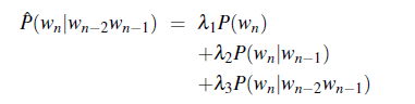
where:

$\sum \lambda_i = 1$, otherwise we can choose the weighting
but we can do better as choosing which one to weight more by context

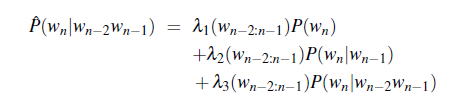
For Example: More sophisticated Linear Interpolation

If we have particularly accurate counts for a particular bigram, we assume that the counts of the trigrams based on this bigram will be more trustworthy, so we can make the ls for those trigrams higher.

i.e. $\lambda$s differ based on which bigram $w_{n-2}w_{n-1}$ we are conditioning on

Then, the parameter $\lambda$ will be huge:

in general, both the simple interpolation and conditional are learned/optimized from a held-out corpus.
- A held-out corpus is an additional training corpus, so-called because we hold it out from the training data, that we use to set hyperparameters like these l values.
- There are various ways to find this optimal set of $\lambda$ s. One way is to use the EM algorithm, an iterative learning algorithm that converges on locally optimal $\lambda$s

Example: Katz backoff

In the end, we want to produce a probability distribution

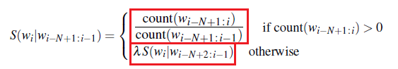
\[P(w_n | w_{n-N+1:n-1})\]

if we naively just do:

\[P(w_n | w_{n-N+1:n-1}) = \begin{cases} P(w_n | w_{n-N+1:n-1}), & \text{if Count}(w_{n-N+1:n}) > 0\\ P(w_n | w_{n-N+2:n-1}), & \text{otherwise} \end{cases}\]

we notice that this will exceed $1$ since just summing up over $P(w_n \vert w_{n-N+1:n-1})$ already reaches $1$.

Therefore, we need to:

discount some probability mass from $P(w_n \vert w_{n-N+1:n-1})$
for lower-order $n$-gram, we need a factor $\alpha$ to distribute it such that everything adds up to 1

\[P_{ \text{BO}}(w_n | w_{n-N+1:n-1}) = \begin{cases} P^*(w_n | w_{n-N+1:n-1}), & \text{if Count}(w_{n-N+1:n}) > 0\\ \alpha ( w_{n-N+1:n-1})\cdot P_{\text{BO}}(w_n | w_{n-N+2:n-1}), & \text{otherwise} \end{cases}\]

where:

we recursively back off to the Katz probability for the shorter-history ($N-1$)-gram if count is zero.
$P^*$ is basically discounted $P$ but also sometimes with smoothing. Commonly used smoothing method here is called Good-Turing.
- The combined Good-Turing backoff algorithm involves quite detailed computation for estimating the Good-Turing smoothing and the $P^*$ and $\alpha$ values

Kneser-Ney Smoothing

One of the most commonly used and best performing n-gram smoothing methods is the interpolated Kneser-Ney algorithm, which has its root from absolute discounting

Absolute discounting is basically, say that given a $n$-gram model and count of each $n$-gram, how much should we discount it so that it is closest to the test dataset?

Recall that discounting of the counts for frequent n-grams is necessary to save some probability mass for the smoothing algorithm

For instance, for a Bigram model, it has been found that the following are the training and heldout dataset

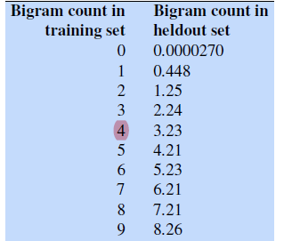
notice that:

if we subtract off $0.75$ for Bigrams with count $2 \sim 9$, it seems to be a pretty close estimate

Therefore, absolute discounting for Bigram models looks like:

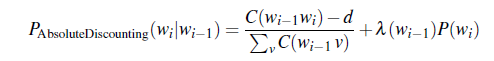
where:

$d$ is the mount you discounted, e.g. $0.75$
the second term is the unigram with an interpolation a conditional weight $\lambda$.

Kneser-Ney discounting (Kneser and Ney, 1995) augments absolute discounting with a more sophisticated way to handle the lower-order unigram distribution.

Essentially instead of blindly picking the most probable $P(w_i)$ if you don’t know what to do next, pick the $w_i$ that is likely to appear in a new/novel context

For instance, consider that you are predicting the next word of:

\[\text{I can’t see without my reading \_\_.}\]

to predict the next word:

if we basically used $P(w_i)$ for interpolation, then words like $\text{Kong}$ might appear more often as a unigram than $\text{glasses}$
basically, if we are only to guess the next word, use the one that appears more context/has a wider distribution
- i.e. $\text{Kong}$ could have only appeared after $\text{Hong}$, but $\text{glasses}$ would have appeared after many different types of words

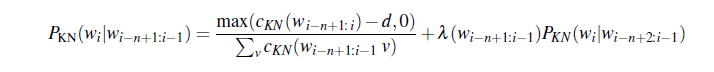
Therefore, we would be doing, for Interpolated Kneser-Ney smoothing for bigrams

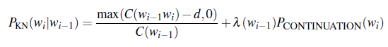
where:

the $\max$ is there since we might go negative in count if $d$ is large
$P_\text{CONTINUATION}$ would be our approximate of how “versatile” a word/phrase would be.

In the case of Bigram, $P_{ \text{CONTINUATION}}$ is formalized as

\[P_{ \text{CONTINUATION}}(w) \propto | \{ v: C(vw) > 0 \}|\]

which is basically the number of word types seen to precede $w$. Then, we need to normalize it, hence

\[P_{ \text{CONTINUATION}}(w) = \frac{ | \{ v: C(vw) > 0 \}|}{\sum_{w'} | \{ v: C(vw') > 0 \}|}\]

so that:

words such as $\text{Kong}$ would have a low continuation probability since it only appears after $\text{Hong}$.

Lastly, a formula for $\lambda$ is also provided

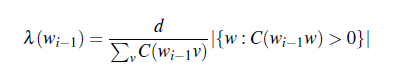
where the first term is basically a normalizing constant

General recursive formulation:

where the definition of the count $c_{KN}$ depends on whether we are

counting the highest-order n-gram being interpolated (for example trigram if we are interpolating trigram, bigram, and unigram)
or one of the lower-order n-grams (bigram or unigram if we are interpolating trigram, bigram, and unigram)

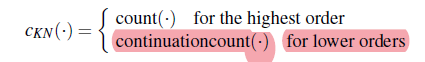
where remember that continuation count is the number of unique single word contexts for $\cdot$.

Huge Web-Scale N-grams

Essentially those huge web-scale data comes from the internet, so we often refer to them as huge web-scale models as well.

Now, efficiency considerations are important when building language models that use such large sets of n-grams

store each string as a 64-bit hash number
Probabilities are generally quantized using only 4-8 bits
n-grams are stored in reverse tries

Other techiniques are used to reduce the size of our model:

Pruning, for example only storing n-grams with counts greater than some threshold

count threshold of 40 used for the Google n-gram release

use entropy to prune less-important n-grams

Bloom filters: approximate language models

All of those are used to improve efficiency of our model when exposed to large corpus

Stupid Backoff

Although with these above toolkits it is possible to build web-scale language models using full Kneser-Ney smoothing, Brants et al. (2007) show that with very large language models a much simpler algorithm may be sufficient.

this algorithm for computing probability is called stupid backoff

Notice that all modifications of the basic N-gram language model is modifying this term:

\[P(w_i | w_{i-n+1:i-1})\]

Stupid backoff basically gives up the idea of trying to make the above quantity a true probability distribution (i.e. sums up to 1).

no discounting of the higher-order probabilities.
simply backoff to a lower order n-gram, weighed by a fixed (context-independent) weight

where, since this is no longer a probability distribution, $S$ instead of $P$ is used:

the upper term is essentially $P(w_i \vert w_{i-n+1:i-1})$
the lower term essentially is a decaying weight the lower n-gram you are using
using $\lambda = 0.4$ seems to work well

Summary

Here we mainly introduced the following techniques/modifications to the basic N-gram model:

smoothing: takes care of the case when word/phrase is unseen
- Add-1/Laplacian Smoothing is easy
- Kneser-Ney works well
backoff and interpolation
- use other probabilities of lower-order n-gram to fill up the gap when count is 0
- require discounting to create a probability distribution
- Kneser-Ney Smoothing: discounting + continuation probability
dealing with large corpus
- efficiency tricks
- stupid backoff: no longer a probability distribution

Spelling Correction

A big task in real life:

Estimates for the frequency of spelling errors in human-typed text vary from 1-2% for carefully retyping already printed text to 10-15% for web queries

The task idea is two fold:

how do you detect spelling errors?
how do you correct spelling errors?
- for correction, some common application uses either autocorrect, suggest a single correction, or suggest a list
together, we call them spelling correction

The task of spelling correction has two broad categories to work with:

non-word spelling correction
real-word spelling correction

Non-word spelling correction is the detection and correction of spelling errors that result in non-words (like graffe for giraffe).

Then, the task involves:

Non-word errors are detected by looking for any word not found in a dictionary. (modern systems often use enormous dictionaries derived from the web.)

corrected by first generate candidates: real words that have a similar letter sequence to the error

Real word spelling correction is the task of detecting and correcting spelling errors even if they accidentally result in an actual real word of English.

due to typographical errors, from insertion/deletion/transposition (e.g., there for three)

due to cognitive errors, substituted the wrong spelling of a homophone or near-homophone (e.g., dessert for desert, or piece for peace).

Then, the task involves:

detection is a much more difficult task, since any word in the input text could be an error

correction will use the noisy channel to find candidates for each word $w$ typed by the user, and rank the correction that is most likely to have been the user’s original intention

the trick is to include the word typed by the user itself in the candidate set

When correcting, both problems will involve the following component:

rank the candidates using a distance metric (e.g. edit distance)
but we also prefer corrections that are more frequent words, or more likely to occur in the context of the error.
- this can then be done by Noisy Channel Model

Noisy Channel

In this section we introduce the noisy channel model and show how to apply it to the task of detecting and correcting spelling errors. An image of what we need to do is the following:

basically the idea is similar to the probabilistic interpretation of logistic regression:

This channel introduces “noise” in the form of substitutions or other changes to the letters, making it hard to recognize the “true” word. i.e.
\[w' = w + \epsilon\]
where $w$ is the word we observe, $w$ is the true word, $\epsilon$ is some random noise we want to model
we need to find the word $w$ that generated this misspelled word $w’$.

Therefore, the idea is clear:

model this noisy channel $\epsilon$
pass every word of the language through our model of the noisy channel
pick the $w$ that comes closest to observed word $w’$

Then, we essentially consider the user input $x$ which is misspelled, but $w$ is the real intention so that:

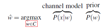
\[x \equiv w' = w + \epsilon\]

We want to find out $\hat{w}$ that is most probably generated $x$:

\[\begin{align*} \hat{w} &= \arg\max_{w \in V} P(w|x)\\ &= \arg\max_{w \in V} \frac{P(x | w)P(w)}{P(x)}\\ &= \arg\max_{w \in V} P(x | w)P(w) \end{align*}\]

then

$P(x\vert w)$ represents the probability a word $w$ generated misspelled $x$ from this noisy channel
- this would be approximated from the training corpus (which contains both a misspelled version and the correct version)
prior probability of a hidden word is modeled by $P(w)$. This represents the probability of seeing the word $w$ at that location/in place of $x$. This hints at us to use Language models such as Bigram, Trigram, etc.

Now, sometimes instead of going over the full dictionary $V$, we can

generating a list of candidate words from $x$, the user input (e.g. misspelled)
use them instead of $V$

Hence the noisy channel model is:

Then the overall algorithm is this:

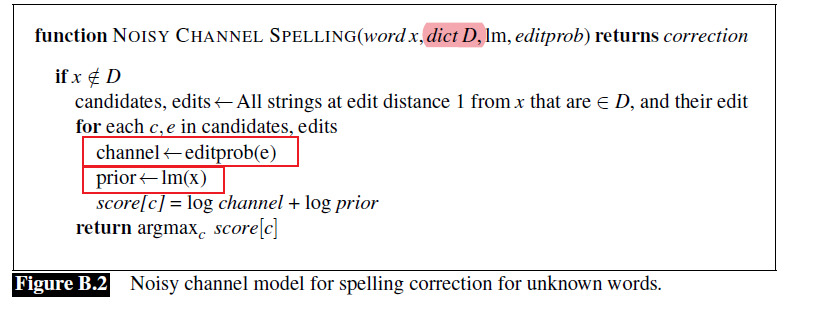
where:

the most important yet haven’t discussed part is how to estimate $P(x\vert w)$, nor $P(w)$ which potentially could depend on many factors such as word context, keyboard position, etc
- prior in general is computed using language model, such as unigram to trigram or 4-gram.
Analysis of spelling error data has shown that the majority of spelling errors consist of a single-letter change and so we often make the simplifying assumption that these candidates have an edit distance of $1$ from the error word
we use extended edit distance so that in addition to insertions, deletions, and substitutions, we’ll add a fourth type of edit, transpositions. This version is also called Damerau-Levenshtein edit distance

Now, we discuss how to estimate the two key probability. We will take the example of correcting the misspelled word “$\text{acress}$”

Estimating $P(x\vert w)$: Simple Model

A perfect model of the probability that a word will be mistyped would condition on all sorts of factors: who the typist was, whether the typist was lefthanded or right-handed, and so on. However, it turns out that we can do pretty well by just looking at the local context.

A simple model might estimate, for example, $P( \text{acress}\vert \text{across})$ just using the number of times that the letter $e$ was substituted for the letter $o$ in some large corpus of errors.

to compute the probability for each edit we’ll need a confusion matrix that contains counts of errors.
In general, a confusion matrix lists the matrix number of times one thing was confused with another.

Then, since we have four operations, we get four confusion matrix, each for:

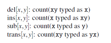
An example for substitution confusion matrix is:

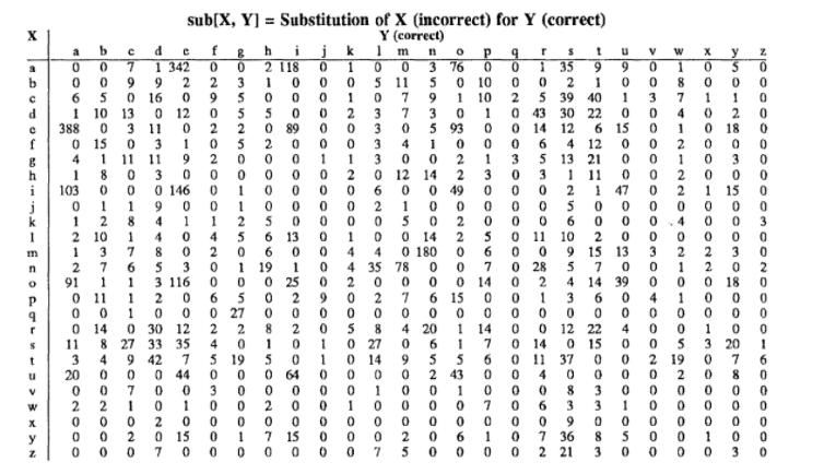
(technically the above is $\text{sub}(y,x)$ by our above definition, but the order is something you can decide by yourself)

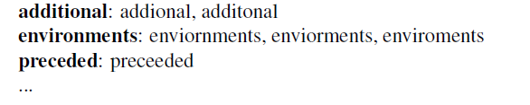
this type of data would be drawn from a list of misspellings like the following
There are lists available on Wikipedia and from Roger Mitton (http://www.dcs.bbk.ac.uk/~ROGER/corpora.html) and Peter Norvig (http://norvig.com/ngrams/).

Finally, with those counts, we can estimate $P(x\vert w)$ as follows:

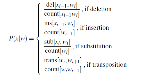
where:

$w_i$ is the $i$th character of the correct word $w$, $x_i$ is the $i$th character of the misspelled word
notice that we are assuming again a single character/operation error, as our candidates are only 1 edit-distance away
notice that we are not caring about the context in this part!

Example computations look like

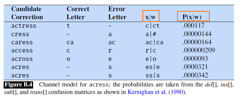
where make sure $x\vert w$ and $P(x\vert w)$ makes sense.

Estimating $P(x\vert w)$: Iterative model

An alternative approach used by Kernighan et al. (1990) is to compute the confusion matrices by iteratively using this very spelling error correction algorithm itself.

The iterative algorithm first initializes the matrices with equal values
- e.g. any character is equally likely to be deleted, etc.
spelling error correction algorithm is run on a set of spelling errors. Given the typos and corrections, update the confusion matrix
repeat step 1

Basically an EM algorithm. Then, once we have the confusion matrix, use the same equation

and the rest is the same.

Estimating $P(w)$: Unigram

Now, recall that our model is:

\[\begin{align*} \hat{w} &= \arg\max_{w \in V} P(w|x)\\ &= \arg\max_{w \in V} \frac{P(x | w)P(w)}{P(x)}\\ &= \arg\max_{w \in V} P(x | w)P(w) \end{align*}\]

so we still need $P(w)$.

If we choose to compute $P(w)$ as a unigram, then:

It turns out $\text{across}$ has a high value!

Unfortunately, this is the wrong choice as the writer’s intention becomes clear from the context:

\[\text{ . . was called a “stellar and versatile \textbf{acress} whose combination of sass and glamour has defined her. . . }\]

The surrounding words make it clear that $\text{actress }$ was the intended word. We are missing context data from unigram + simple model for $P(x\vert w)$ based on purely alphabets.

Estimating $P(w)$: Bigram

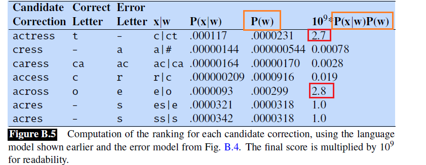
Now, with bigram, we can compute $P(\text{actress})$ and $P(\text{across})$ as:

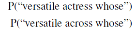
which then can be estimated using bigram because we know the following:

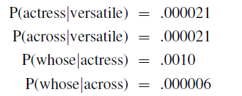
Finally:

which combining the the $P(x\vert w)$ prediction, we gave out the correct result that $\text{actress}$ is more likely.

Real-Word Spelling Errors

Recall that another class of problem is that we might have mistyped but those words exist.

The noisy channel approach can also be applied to detect and correct those errors as well! But we need a small tweak.
A number of studies suggest that between 25% and 40% of spelling errors are valid English words

For instance:

\[\text{This used to belong to \textbf{thew} queen. They are leaving in about fifteen \textbf{minuets} to go to her house.}\]

How do we use noisy channel that seems to be based on detecting error from misspelling?

Let’s begin with a version of the noisy channel model first proposed by Mays et al. (1991) to deal with these real-word spelling errors.

Idea:

takes the input sentence $X = {x1 , x_2 , …, x_n }$

Generates a large set of candidate correction sentences $C(X)$

start by generating a set of candidate words $C(x_i)$ for each input word $x_i$, e.g. within edit distance 1

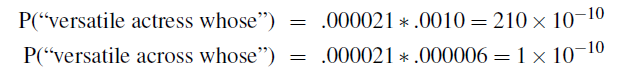
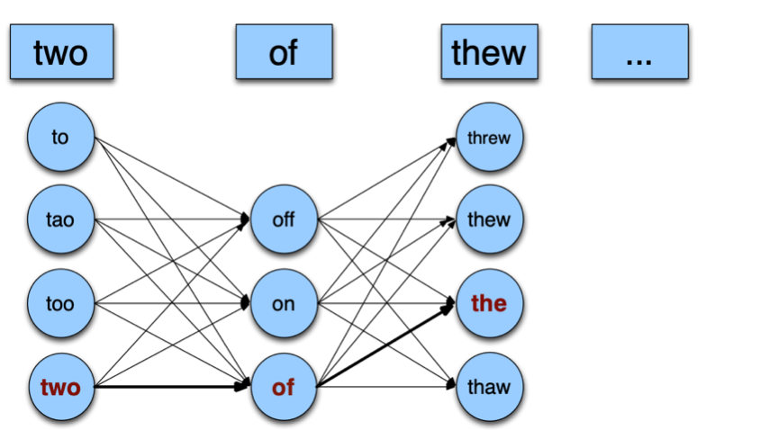
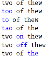
generate possible sentences from those words. For instance, if the input is $\text{two of thew}$:

where we already see a lot of possibility. To simplify, we assume that every sentence has only one error. Then we have:

picks the sentence with the highest language model probability
\[\hat{W} = \arg\max_{W \in C(X)} P(W|X)= \arg \max_{W \in C(X)} P(X|W)P(W)\]
where $W$ we know are generated by us.

Now, the problem is we need to estimate:

$P(X\vert W)$
$P(W)$ - this can be done using a language model, essentially like we are generating sentences from it. (e.g. use a Trigram)

Now, the problem is $P(X\vert W)$. Since we assume only one word error, then we can assume:

\[P(X|W) = P(x_1, ..., x_n | w_1, ..., w_n) = \prod_{i=1}^n P(x_i|w_i)\]

where we assumed each $x_i\vert w_i$ pair are uncorrelated to each other. Then, if correct, i.e. $x_i = w_i$, we assumed $\alpha$ (as shown below). Hence:

\[P(X|W) = \prod_{i=1}^n P(x_i|w_i) = \alpha^{n-1}P(x_k|w_k)\]

where:

we assumed there is only one error, and the error is on $x_k$.

since context information/positional information is encoded into $P(W)$. Then, we can use the simple model that

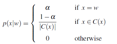
where notice that:

essentially $P(w\vert w)$, i.e. typed correctly, is probability $\alpha$. Often this is set to $\alpha = 0.95$
alternatively we can make the distribution proportional to the edit probability from the more sophisticated channel model. i.e. we use $P(x\vert w)$ estimation by look at the confusion matrices.

Lastly, since constants can be dropped during $\arg\max_W$:

\[\hat{W} =\arg \max_{W \in C(X)} P(X|W)P(W) = \text{arg\,max}_{W \in C(X), k\in[1,n]} P(x_k|w_k)P(W)\]

for the single wrong word being at position $k$.

For example, if we used the simple estimation for $P(x\vert w)$, then $P(X\vert W)$ essentially is:

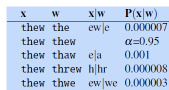
where here we only looked at the case when we want to correct $\text{thew}$ in the sentence, which again is a real word.

finally, don’t forget to multiply by $P(W)$ to get your final estimate for $P(W\vert X)$!

Noisy Channel Model: The State of the Art

State of the art implementations of noisy channel spelling correction make a number of extensions to the simple models we presented above. Here we go over a few

rather than make the assumption that the input sentence has only a single error, modern systems go through the input one word at a time, using the noisy channel to make a decision for that word.
we could suffer from overcorrecting, replacing correct but rare words with more frequent words
- Google solves this by using a blacklist, forbidding certain tokens (like numbers, punctuation, and single letter words) from being changed
- Instead of just choosing a candidate correction if it has a higher probability $P(w\vert x)$ than the word itself, these more careful systems choose to suggest a correction $w$ over keeping the non-correction $x$ only if the difference in probabilities is sufficiently great.
improve the performance of the noisy channel model by changing how the prior and the likelihood are combined
- we might trust one of the two models more, therefore we use a weighted combination
  \[\hat{w} = \arg\max_{w \in V} P(x|w)P(w)^\lambda\]
  for some constant $\lambda$
For specific confusion sets, such as peace/piece, affect/effect, weather/whether, we can train supervised classifiers to draw on many features of the context and make a choice between the two candidates
- achieve very high accuracy for these specific set
- but it requires some handcrafted feature extraction/work
Since many documents are typed, error by nearby keys include more weights
- for instance, used in weighing edit distance

Neural Networks in NLP

Basically the same content as ML: review Perceptron. This include:

how the does the update rule in a single perceptron work?
perceptron as a linear classifier
(maybe checkout SVM)

In DL, review the chapter of Neural Network and Backpropagation.

feed-forward network
activation functions
backpropagation
- this will be tested on Midterm

Architecture for Neural Language Model

Now, let’s talk about the architecture for training a neural language model

Comments on Model/Training

Comments on Training

Many epochs (thousands) may be required, hours or days of training for large networks.
To avoid local-minima problems, run several trials starting with different random weights (random restarts).
- Take results of trial with lowest training set error.
- Build a committee of results from multiple trials (possibly weighting votes by training set accuracy).
Keep a hold-out validation set and test accuracy on it after every epoch.
- Stop training when overfitting. Do callbacks/epoch saves

Comments on Model/Architecture choice:

Trained hidden units can be seen as newly constructed features that make the target concept linearly separable in the transformed space. (e.g. for CNNs, edges, textures, etc.)
- However, the hidden layer can also become a distributed representation of the input in which each individual unit is not easily interpretable as a meaningful feature.
Too few hidden units prevents the network from adequately fitting the data, but too many hidden units can result in over-fitting.
- Use internal cross-validation to empirically determine an optimal number of hidden units.

RNN and LSTM

For RNN:

review DL notes, on the section of Sequence Models.

Recall

The basic problem of RNN (e.g. Deep RNN or stacked RNN) is that backpropagation involves matrices multiple times. This will cause the problem of vanishing/exploding gradient

difficult to train a RNN

Some ideas to solve this problem:

LTSM
GRU

Both of which will also be able to model long term dependencies

Transformers

Essentially you have:

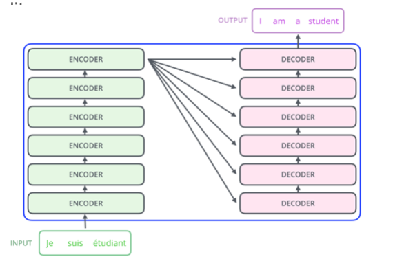
where:

many stacked layers of encoder and stacked layers of decoder
- an encoder essentially is a transformer block
input to the decoder only comes form the last layer

Within each encoder, essentially you will have:

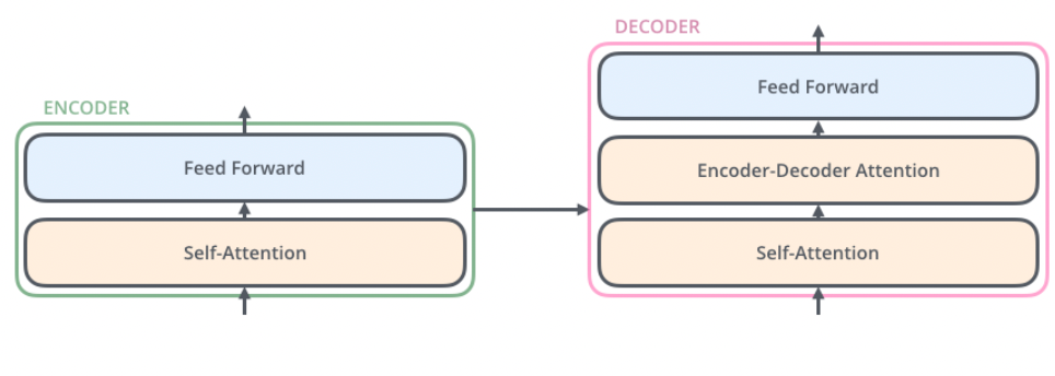
where:

feed forward layer basically is a NN that feeds forward (layers of linear + nonlinear activation)

Checkout the Transformer section in the DL notes.

Transformer Models

Essentially different models use different number of stacks for encoder/decoder/attention

Models are larger and larger
More computation resources are required
Models example: GPT, BERT, Roberta, T-5

Vector Semantics and Embeddings

This chapter essentially deals with how we represent texts as vectors.

In more detail, we will use the distributional hypothesis that “words that occur in similar contexts tend to have similar meanings.” to instantiate this linguistic hypothesis, we will see this done by learning representations of the meaning of words, called embeddings. We will cover:

static embeddings (e.g. SGNS Embedding from Word2Vec)
contextualized embeddings (e.g. BERT)

All of those are done by self-supervised ways to learn representations of the input.

Lexical Semantics

The idea is that we want to compute similarity between words, i.e. a vector representation that achieves this.

Lexical Semantics is the study of word meanings. It includes the study of how words structure their meaning, how they act in grammar and compositionality, and the relationships between the distinct senses

First of all, recall some terms commonly used in NLP include:

lemma, basically the “infinitive” form of words, such as “sing”
wordforms, the specific form of words, such as “sings, sang”
word sense: aspect of meaning of a word (e.g. a word could have many meanings)

Some of the important aspects we need to answer for representing words include:

Word Similarity: being able to measure similarity between two words is an important component of tasks like question answering, paraphrasing, and summarization
- e.g. synonyms would have high similarity
- but also words such as “cat/dog” would have high similarity
Word Relatedness: the meaning of two words can be related in the sense of association
- e.g. the word coffee and the word cup are very related yet have different meanings
- One common kind of relatedness between words is if they belong to the same semantic field
  - For example, words might be related by being in the semantic field of hospitals (surgeon, scalpel, nurse, anesthetic, hospital)
Semantic Frames and Roles: a set of words that denote perspectives or participants in a particular type of event
- e.g. understanding a sentence like Sam bought the book from Ling could be paraphrased as Ling sold the book to Sam, and that Sam has the role of the buyer in the frame and Ling the seller
Connotation: aspects of a word’s meaning that are related to a writer or reader’s emotions, sentiment, opinions, or evaluations. Hence very related to sentiment analysis of texts!

Early work on affective meaning (Osgood et al., 1957) found that words varied along three important dimensions of affective meaning:
- valence: the pleasantness of the stimulus
- arousal: the intensity of emotion provoked by the stimulus
- dominance: the degree of control exerted by the stimulus
Then, we can represent a word by a 3D vector, each component a score for each of the above. With this, we introduce the revolutionary idea of word embedding - represent words as vectors!

Vector Semantics

Vectors semantics is the standard way to represent word meaning in NLP, essentially helping us to build models that takes in texts.

In short, we will consider the merging the idea of:

representing a word as a vector (e.g. in 3D space)
define the meaning of a word by its distribution in language use, meaning its neighboring words or grammatical environments

Therefore, our task is to represent a word as a point in a multidimensional semantic space that is derived (in ways we’ll see) from the distributions of embeddings word neighbors.

Vectors for representing words are called embeddings (although the term is sometimes more strictly applied only to dense vectors like word2vec (Section 6.8), rather than sparse TF-IDF or PPMI vectors

In this chapter we will mainly discuss two commonly used models

TF-IDF, which is usually used as the baseline, consider the meaning of a word is defined by a simple function of the counts of nearby word
- hence, resulting in sparse vectors
Word2Vec, which is technically a family of algorithms that construct short, dense vectors that have useful semantic properties

(We’ll also introduce the cosine, the standard way to use embeddings to compute semantic similarity, between two words, two sentences, or two documents, an important tool in practical applications like question answering, summarization, or automatic essay grading)

Words and Vectors

Vector or distributional models of meaning (mentioned above) are generally based on a co-occurrence matrix, a way of representing how often words co-occur. Two popular matrices related to this is:

term-document matrix
term-term matrix

Vectors and Documents

In Term-document matrix, each row represents a word in the vocabulary and each column represents a document from some collection of documents

e.g. a document could be a book

Then, the value would be number of times a particular word (defined by the row) occurs in a particular document (defined by the column).

For example, term frequency would look like:

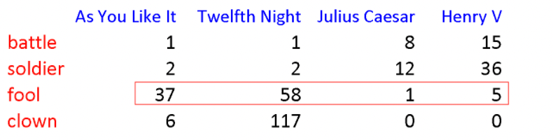
where:

notice that each row could be treated as a vector for the word!
similarly (but maybe not that useful for now), a document can then be represented as a column vector
- interestingly, this idea was introduced as as means of finding similar documents for the task of document information retrieval, i.e. having similar column vectors

This can be useful to determine similarity between word if their vector representation is similar

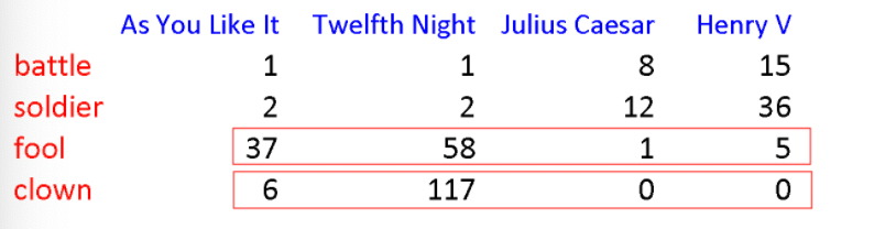
for instance, “fool” and “clown” would be more similar than others.

a problem with this is that we need lots of documents to represent more accurate information
vocabulary sizes are generally in the tens of thousands, and the number of documents can be enormous (think about all the pages on the web). Hence the size of the matrix will also be enormous!

Term-Context Matrix

An alternative to using the term-document matrix to represent words as vectors of document counts, is to use the term-term matrix, also called the word-word matrix or term-context matrix

In term-context matrix: columns are labeled by words rather matrix than documents.

This matrix is thus of dimensionality $\vert V\vert \times \vert V\vert$

each cell records the number of times the row (target) word and the column (context) word co-occur in some context in some training corpus

e.g. the context could be the document, in which case the cell represents the number of times the two words appear in the same document.

It is most common, however, to use smaller contexts, generally a window around the word, for example of 4 words to the left and 4 words to the right

For instance, consider the following training corpus:

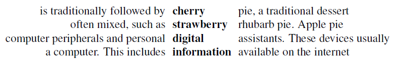
we want to compute the term-context matrix for the target word highlighted in bold.

where we are taking a window size of $\pm 7$ for context word.

Then, if we take every occurrence of each word (say strawberry) and count the context words around it, we get a word-word co-occurrence matrix:

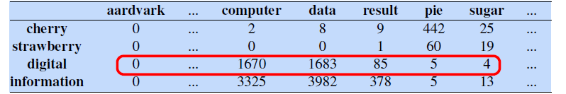
note that:

here, the words cherry and strawberry are more similar to each other, and the same goes for digital and information
therefore, if the vector for a word is close to each other, we would expect the row vector to look similar (the column vector would be a context vector, which we can choose to ignore in this case)
in general, the shorter the window size captures more syntactic representation, and the longer the window, the more semantic representation (e.g. $L=4\sim 10$)

However, this is problematic in reality because if we have vocabulary size of $50,000$, then this means that the matrix will have dimension $\mathbb{R}^{50,000 \times 50,000}$, and it will be sparse!

TF-IDF

The co-occurrence matrices above represent each cell by frequencies, either of words with documents (Fig. 6.5), or words with other word. But raw frequency does not work directly:

want to know what kinds of contexts are shared by cherry and strawberry but not by digital and information. But there are words that occur frequently with all sorts of words and aren’t informative about any particular word (e.g the, good, etc)
essentially, words that occur too frequent are sometimes unimportant, e.g. good

Therefore, the solution is to somehow add weighting (essentially the idea of TF-IDF and PPMI as well)

TF-IDF essentially consist of two components:

term frequency in log, essentially captures the frequency of words occurring in a document (i.e. the word-document matrix)

inverse document frequency, essentially giving a higher weight to words that occur only in a few documents (i.e. they would carry important discriminative meanings)

The term frequency in a document $d$ is computed by:

\[\text{tf}(t,d) = \log_{10}(\text{count}(t,d) + 1)\]

where:

we added $1$ so that we won’t do $\log 0$, which is negative infinity

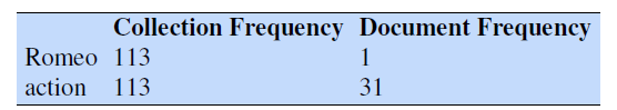
The document frequency of a term $t$ is the number of documents it occurs in.

note that this is different from collection frequency of a term, which is the total number of times the word appears in any document of the whole collection

For example: consider in the collection of Shakespeare’s 37 plays the two words Romeo and action

Therefore, we want to emphasize discriminative words like Romeo via the inverse document frequency or IDF term weight:

\[\text{idf}(t) = \log_{10}\left( \frac{N}{\text{df}(t) } \right)\]

where:

apparently $\text{df(t)}$ is the number of documents in which term t occurs and $N$ is the total number of documents in the collection
so essentially, the fewer documents in which a term occurs, the higher this weight.
notice that we don’t need $+1$ here because the minimum document frequency of a word in your corpus would be $1$
again, because the number could be large, we use a $\log$.

Here are some IDF values for some words in the Shakespeare corpus

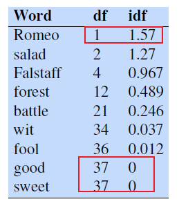
so we have:

extremely informative words which occur in only one play like Romeo
those that occur in a few like salad or Falstaff
those which are very common like fool
so common as to be completely non-discriminative since they occur in all 37 plays like good or sweet

Finally, the TF-IDF basically then does:

\[\text{TF-IDF}(t,d) = \text{tf}(t,d) \times \text{idf}(t)\]

An example would be:

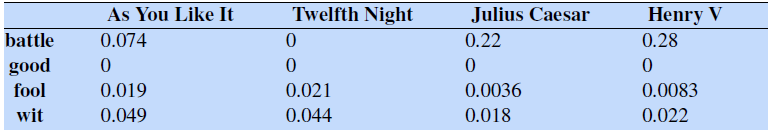
where notice that:

essentially it is still a term-document matrix, but it is weighted by IDF.
notice that because $\text{idf(good)}=0$, the row vector for good becomes all zero: this word appears in every document, the tf-idf weighting leads it to be ignored (as it is not very informative anymore)

Note

this is by far the most common weighting metric used when we are considering relationships of words to documents

however, not generally used for word-word similarity, which PPMI would be better at

PPMI

An alternative for TF-IDF would be PPMI (positive pointwise mutual information), which is essentially weightings for term-term-matrices.

Intuition:

PPMI considers the best way to weigh the association between two words is to ask how much more often the two words co-occur in our corpus than we would have a priori expected them to appear by chance

i.e. like a ratio of them appearing by chance v.s. actually appearing together in our corpus

Therefore, this is a measure of how often two events $x$ and $y$ occur, compared with what we would expect if they were independent:

\[I(x,y) = \log_2\left(\frac{P(x,y)}{P(x)P(y)}\right)\]

where essentially:

probability of them occurring jointly together over them occurring independently

Hence, the pointwise mutual information between a target word $w$ and a context word $c$ (Church and Hanks 1989, Church and Hanks 1990) is then defined as:

\[\text{PMI}(w,c) = \log_2\left(\frac{P(w,c)}{P(w)P(c)}\right)\]

where notice that:

since we are back with word-context matrix, we consider target words $w$ and context $c$
each probability would then be estimated by MLE, which basically are counts
the denominator computes the probability that the two words to co-occur assuming they each occurred independently, the numerator of will be them actually co-occurring
therefore, it is a useful tool whenever we need to find words that are strongly associated
PMI values ranges from negative to positive infinity

Now, in reality, the problem with PMI is that negative PMI values (which imply things are co-occurring less often than we would expect by chance) tend to be unreliable unless our corpora are enormous.

To distinguish whether two words whose individual probability is each $10^{-6}$ occur together less often than chance, we would need to be certain that the probability of the two occurring together is significantly different than $10^{-12}$, and this kind of granularity would require an enormous corpus.

Therefore, we often turn to the Positive PMI (PPMI), which replaces all negative PMI values with zero:

\[\text{PPMI}(w,c) = \max\left( \log_2 \frac{P(w,c)}{P(w)P(c)},0 \right)\]

More formally, for our word-context matrix $F$, if we have $W$ rows (words) and $C$ columns (contexts), and each element is represented by $f_{ij}$, we can estimate the probability by:

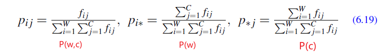
Therefore, the PPMI can be computed as:

\[\text{PPMI}(w,c) = \max\left( \log_2 \frac{p_{ij}}{p_{i*}p_{*j}},0 \right)\]

For Example

Consider the following given statistics:

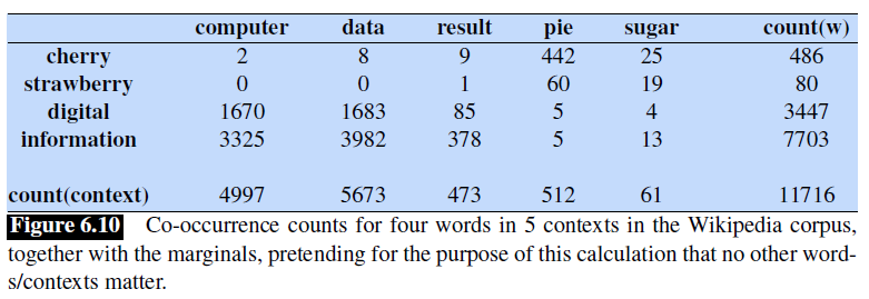
we could compute $\text{PPMI(information,data)}$, assuming we pretended that Fig. 6.6 encompassed all the relevant word contexts/dimensions, as follows:

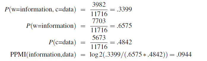
Alternatively, notice that essentially the above probabilities are joint and their marginal. So, we can compute the joint $P(w,c)$ with their marginal shown on the right/bottom:

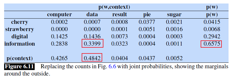
where you see the three values are exactly what we used before for PPMI.

Lastly, doing it for all pairs results in:

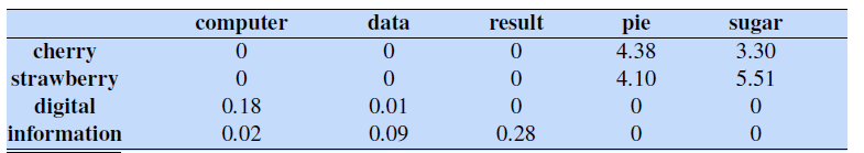
so we see that:

cherry and strawberry are highly associated with both pie and sugar
data is mildly associated with information

Weighted PMI

PMI is biased toward infrequent events

Very rare words have very high PMI values, as $P(c)$ could be low

Two solutions:

Give rare words slightly higher probabilities (covered here)
Use add-one smoothing (covered next)

Therefore, now we consider:

\[\text{PPMI}(w,c) = \max\left( \log_2 \frac{P(w,c)}{P(w)P_\alpha(c)},0 \right)\]

for:

\[P_\alpha (c) = \frac{\text{Count}(c)^\alpha}{\sum_c \text{Count}(c)^\alpha}\]

for some $\alpha < 1$, so that $P(c)$ is larger for rare words.

empirically using $\alpha = 0.75$ works pretty well

Laplace Smoothing

Another way to get rid of the problem is to do add-k smoothing:

Before computing PMI, a small constant $k$ (values of 0.1-3 are common) is added to each of the counts:

For instance

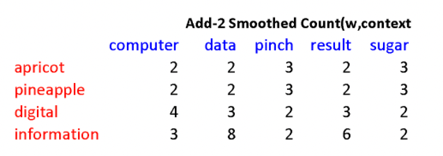
Then, the rest of the computation is the same:

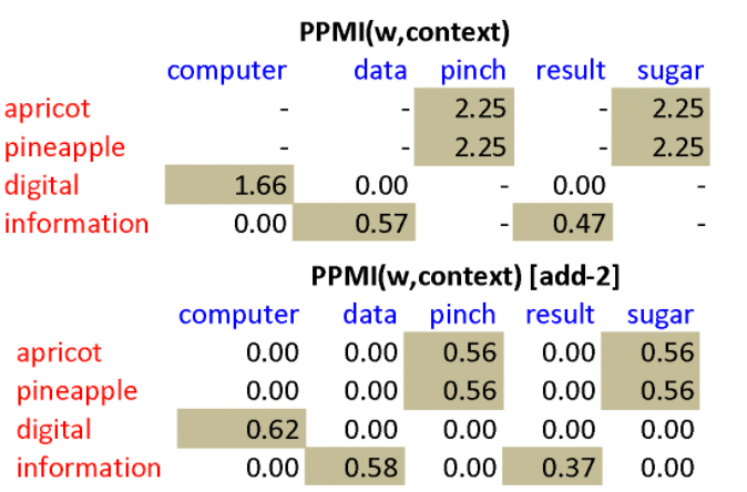
Cosine Distance

Now, after all the above of embedding, we return to the task of measuring properties such as similarities between two embeddings:

To measure similarity between two target words $v$ and $w$, we need a metric that takes two vectors and spit out some values
By far the most common similarity metric is the cosine of the angle between the vectors (i.e. normalized dot product)

Why can we not use raw dot product?

the raw dot product favors long vectors, or with high values in each dimension, as it is just a sum.

We do not want that because more frequent words have longer vectors, since they tend to co-occur with more words and have higher co-occurrence values with each of them

we’d like a similarity metric that tells us how similar two words are regardless of their frequency

Therefore, we would like to be able to normalize them. Then, essentially we get a cosine of the angle:

\[\frac{a \cdot b}{|a||b|} = \cos(\theta_{ab})\]

where:

we can use the $v,w$ vector being the PPMI vector for word $v$, or TF-IDF vectors, or whatever we want

For Example: Raw Frequency Count

If we have a raw frequency count word-context matrix, such that each word embedding is essentially a row vector:

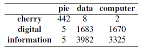
Then, we can compute, for instance the similarity between cheery and information v.s. digital and information

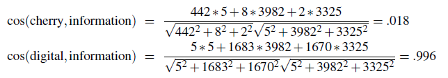
where the result here makes sense because information is indeed more similar to digital then cherry!

For Example: Document Similarity

One way to measure similarity between documents is to use the document vector (if you have), and consider the cosine similarity between them. However, here we introduce another idea:

for $k$ words in a document, consider the embedding for each word $w_i$
then, compute the centroid to be representing the document:
\[d = \frac{w_1 + w_2 + ... + w_k}{k}\]
compute $\cos(d_1,d_2)$ of the angles to measure similarly.

Other Similarity Measures

Besides cosine similarly, some other common ones are shown below:

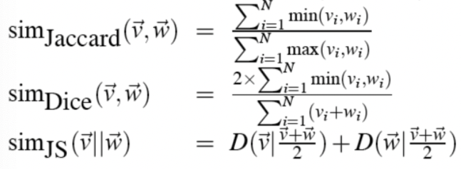
Using Syntax

Before, we cared more about semantics as a measure of similarity. Now, we consider words are similar if they have similar syntactic contexts.

for example, we can count syntax occurance instance of just word occurance:
\[\text{M(“cell”,”absorb”) = count(subj(cell,absorb)) + count(obj(cell,absorb)) + ...}\]

Then, we can also construct a frequency matrix where the values represent count syntax occurrence. With that, we can then compute quantities such as PMI:

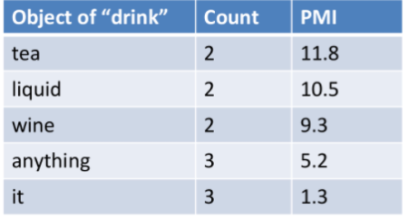
where in this example, we see that:

drink tea and drink liquid is more associated (syntactically) to each other than drink it, for instance

Word Embeddings

We see that the previous examples:

PPMI and context vectors are all sparse vectors
we want to save space/encode information by a dense vector - which is often called the word embedding

Some common techniques to obtain a dense representation would be:

SVD/PCA/Factor Analysis of the PPMI matrix, or TF-IDF embedding matrix
- since in SVD we can choose to only include the top $k$ eigenvalues, we can essentially reduce dimension to $k$
Neural Language Model, embedding using ML
- e.g. skip-gram, using Machine Learning models to train/output embedding matrix
Brown Clustering

SVD

will not be on the exam

Goal:

Approximate an N-dimensional co-occurrence matrix or whatever matrix you like using fewer dimensions.

Recall that:

Let $A \in \mathbb{R}^{n \times p}$. Then:

\[A = USV^T\]

is the singular value decomposition where:

$U^TU=I \in \mathbb{R}^{n \times n}$, and $V^TV=I \in \mathbb{R}^{p \times p}$
The eigenvectors of $A^TA$ make up the columns of $V$ , the eigenvectors of $AA^T$ make up the columns of $U$
singular values in $S$ are square roots of eigenvalues from $AA^T$ or $A^TA$

To begin with, consider the matrix we want to truncate is $X$:

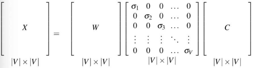
Then, since we want to truncate the dimension, we would like to have embedding matrix of size $\vert V\vert \times k$, hence we consider taking only the $k$ singular values

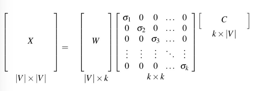
Then we can treat:

$W$ matrix for the embedding matrix, $C$ be the context matrix, both of which now has only vectors of dimension $k$
the reason why we take $W$ which is essentially the matrix $U$ in $A=USV^T$ is related to the PCA understanding covered next

PCA

The PCA viewpoint requires that one compute the eigenvalues and eigenvectors of the covariance matrix, which is the product:

\[\frac{1}{n-1} XX^T = \frac{1}{n-1}WDW^T\]

where recall that covariance matrices are symmetric.

$X$ is the matrix where we want to decompose
then, we will take the principle axis in $D$ to embed data

Its relation to SVD can be seen easily if we consider:

\[X= USV^T\]

then reconstructing the covariance:

\[\frac{1}{n-1}XX^T = \frac{1}{n-1}(USV^T)(USV^T) = \frac{1}{n-1}US^2U^T\]

where it is obvious that:

$U \to W$ is the correspondence between SVD and PCA, also related to why we are taking $W$ to be the word matrix in the above section.

Skip-Gram Embedding

Some advantage using ML related algorithms for embedding

much faster to train than methods such as SVD
better performance
(skip-gram algorithm is one word2vec of two algorithms in a software package called word2vec)

Intuition

We’re going to train a simple neural network with a single hidden layer to perform a certain task:

but then we’re not actually going to use that neural network for the task we trained it on!

Instead, the goal is actually just to learn the weights of the hidden layer - we’ll see that these weights are actually the “word embeddings” that we’re trying to learn.

Additionally:

this can be done in self-supervision, which avoids the need for any sort of hand-labeled supervision signal

this is static, in that it learns one fixed embedding for each word in the embeddings vocabulary.

In the Transformer chapter in DL notes, we will introduce methods for learning dynamic contextual embeddings like the popular family of BERT representations, in which the vector for each word is different in different contexts

This model then can be extended to include negative samplings, which is covered next.

The goal of our simple neural model is this (e.g. say out vocabulary size is $\vert V\vert$)

given an input target word (e.g. Soviet)
- also perhaps specify a window size (e.g. $L=5$)
- input will be a one-hot encoded vector of dimension $\vert V\vert$
output probability for each word $w_i \in V$ to be next to the input word, within the specified window
- e.g. output probabilities are going to be much higher for words like “Union” and “Russia” than for unrelated words like “watermelon” and “kangaroo”.
- output will also be vector of dimension $\vert V\vert$, but values are the probability that word will be inside the window
We’ll run the model once per context word within the window defined by $L$

Then, our architecture this the follows, say that $\vert V\vert =10,000$:

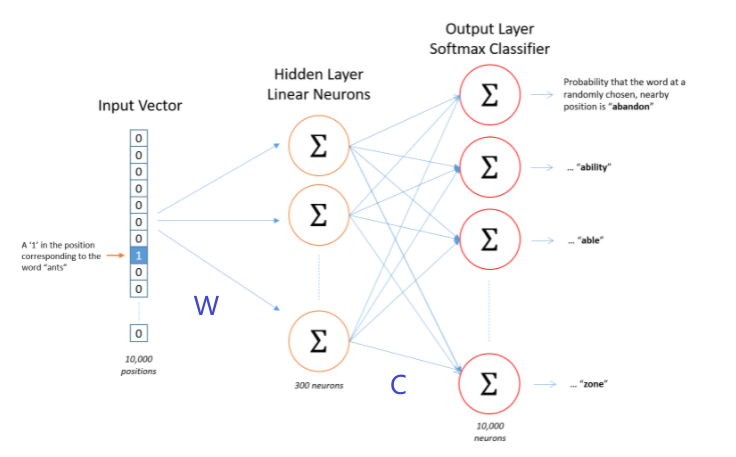
where we have:

$W \in \mathbb{R}^{\vert V\vert \times d}$ so that the first layer is $W^T x_t = e_t$ for the $t$-th word
$C \in \mathbb{R}^{d \times \vert V\vert }$ so that the output layer does:
\[o = \text{Softmax}(C^T e_t) \in \mathbb{R}^{|V|\times 1}\]
is essentially the probability for each word in the vocabulary as a neighbor to $w_t$
finally, since we need to output probability, we take SoftMax as the activation layer in the end
graphically, the two matrices loko like:

$W$ $C$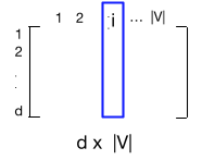

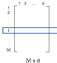
where we can see that:
- the $e_i = W^T x_i$ for one-hot vector $x_i$ shows that the $i$-th column of $W$ is the word/input embedding for word $w_i$
- then $o[k] \propto C^Te_i[k]$ for an embedded target word $w_i$ means the $k$-th row of $C$ is the context embedding of $w_k$ relative to $w_i$ being the target

Therefore, interpretation of the output would be:

\[p(w_k | w_t) = \frac{\exp(c_k \cdot e_t)}{\sum_{k \in |V|} \exp(c_k \cdot e_t)}\]

is like a bigram probability, but here it signified the probability of word $w_k$ being within the window of $w_t$.

Finally, we need to define a loss. Our objective is to maximize the probability of the entire sentence.

\[\begin{align*} &\quad\arg\max_\theta \prod_{t=1}^T P(w_{t-L},...,w_{t-1},w_{t+1},...,w_{t+L})\\ &=\arg\max_\theta \prod_{t=1}^T \prod_{-L \le j \le L, j \neq 0} P(w_{t+j}|w_t;\theta)\\ &=\arg\min_\theta -\sum_{t=1}^T \sum_{-L \le j \le L, j \neq 0} \log P(w_{t+j}|w_t;\theta) \end{align*}\]

note that:

$T$ is the length of the entire sequence/sentence, $L$ is the window size
essentially this is negative loss likelihood, which is the same as cross entropy loss, which recall is basically the loss if you used $q(x)$ to approximate $p(x)$:

\[H(p,q) = -\sum_x p(x)\log q(x)\]

Then, we abasically obtained two embedding matrix $W,C$:

either just use $W$ as our embedding matrix
use $W+C^T$
use $[W,C^T]$ by concatenating

Note

It turns out that this simple skipgram is very related to PPMI matrix

$WC^T \in \mathbb{R}^{\vert V\vert \times \vert V\vert }$ can be shown as:
\[WC^T = M_{PPMI}- \log k\]
so that each element in $WC^T$ is related to association between input $i$ and output word $j$.

Training:

Training data comes by feeding it word pairs found in our training documents

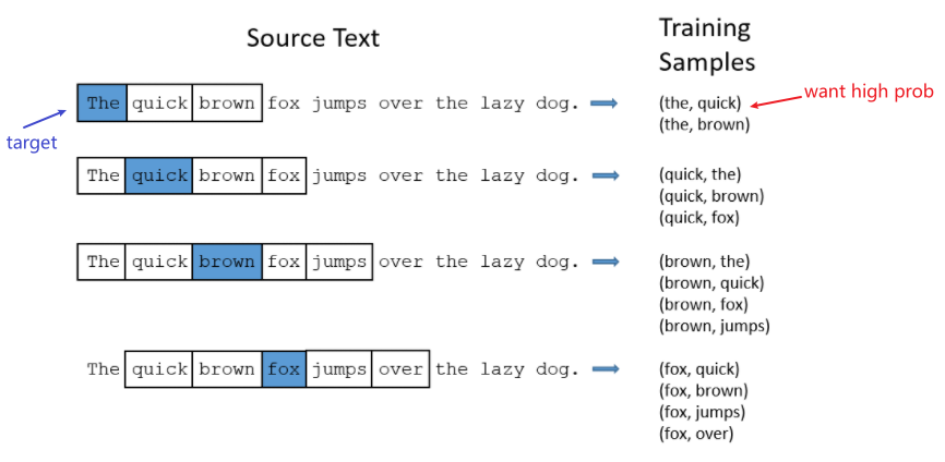
then use gradient descent to minimize the loss. In this example a window size of $L=2$ is used.

SGNS Embeddings

In this section we introduce one method for computing embeddings: skip-gram SGNS with negative sampling, sometimes called SGNS.

the previous version only included positive samples

Intuition

The intuition of word2vec is to train a classifier on a binary prediction task: given a word $w$, how likely is it to show up near another word $w_i$, e.g. apricot?

essentially training a logistic regression classifier

however, now we also try to include negative samples to make our model/embedding more robust

Then, while we are learning the likelihood, we would have needed/learnt some representation $\vec{w}$ for a word $w$, which will be our embedding!

Therefore, the model is simple:

Treat the target word $w$ and a neighboring context word as positive examples.
Randomly sample other words in the lexicon to get negative samples.
Use logistic regression to train a classifier to distinguish those two cases.
Use the learned weights $W$ as the embeddings, commonly represented as $E$

Note

This means that the embedding for word $w_i$ will be similar to $w_j$ if they are physically close to each other.

i.e. if phrases like “bitter sweet” will create problems in the embedding! (physically close but their meanings are different)

SGNS Classifier

Goal of Classifier:

Given a tuple $w,c$ being target word $w$ paired with a candidate word $c$, what is the probability that $c$ is a context word (i.e. physically next to it)?

To present such probability, we will use:
\[P(+|w,c) = \sigma(\vec{w}\cdot \vec{c}) =\frac{1}{1 + \exp(-\vec{w}\cdot \vec{c})}\]
for $\vec{w},\vec{c}$ being the embedding of word $w,c$.

so on our way to learn such classifier, we would have learnt $\vec{w},\vec{c}$ which will be used for embedding

Consider we want to find out the embedding of the word $\text{apricot}$, and we have the following data:

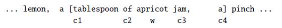
where:

let us take a window size of $2$, so that we view $[c_1, …, c_4]$ above as real context word for $\text{apricot}$.
our goal is to have a logistic regression such that:
\[P(+|w,c)\]
is high if $c$ is a real context word, and that:
\[P(-|w,c) = 1-P(+|w,c)\]
is high if $c$ is not a context word.

Then, the question is how do we model such probability? We assumed that words next to each other should have similar embeddings. This means that:

\[\text{Similarity}(w,c) \approx \vec{w} \cdot \vec{c}\]

for $\vec{w},\vec{c}$ being the embeddings for the word $w,c$. Then, to map this to probability that $c$ is a real context word for $w$ as:

\[P(+|w,c) = \sigma(\vec{w}\cdot \vec{c}) =\frac{1}{1 + \exp(-\vec{w}\cdot \vec{c})}\]

is high if high dot product = similar = next to each other. Then similarly, probability that $c$ is not a context word as:

\[P(-|w,c) = \sigma(-\vec{w}\cdot \vec{c}) =\frac{1}{1 + \exp(+\vec{w}\cdot \vec{c})}\]

for $c$ being negative samples (not context words).

Now, this means that we can also assign “similarity score” between a target word and a context window:

\[P(+|w, c_{1:L}) = \prod_{i=1}^L \sigma(\vec{c}_i \cdot \vec{w})\]

where:

we assumed all contexts words are independent
we can also compute the log probability to make it a sum

Now, we can think of what are are learning graphically:

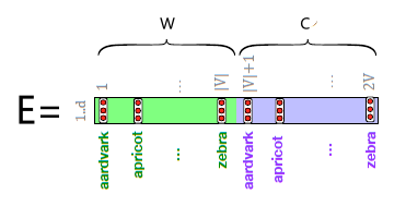
where essentially:

Embedding matrix $E$ contains two matrices, $W$ for word embedding and $C$ for context embedding
- i.e. for the $i$-th word (in the dictionary), its word embedding will be the $i$-th column of $W$, and similarly for context embedding
- i.e. every word will have two embeddings, one in $W$ and another in $C$. In reality people either only take $W$ or take $W+C$
- if your vocabulary size is $\vert V\vert$, and you want an embedding of dimension $d$, then $W,C \in \mathbb{R}^{d \times \vert V\vert }$ so that you can fetch the embedding from a one-hot vector.
we have two embeddings because a word $w$ could be treated as a target, but sometimes it might also be picked as a context $c$, in which we update the embedding separately.

Learning the Embedding

Our target is to learn the matrix:

Let us begin with an example text, where our target word currently is $w=\text{apricot}$.

Then taking a window size of $2$, we also want to have negative samples (in fact, more negative samples than positive ones per target word so that we are called SGNS):

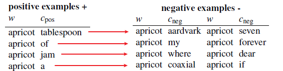
where here:

each of the training sample $(w, c_{pos})$ comes with $k=2$ negative samples, for $k$ being tunable
the negative samples are sampled randomly by:
\[\text{Prob of sampling $w$}= P_\alpha(w) = \frac{ \text{Count}(w)^\alpha }{\sum_{w'} \text{Count}(w')^\alpha}\]
where we usually take $\alpha = 0.75$ so that rare words have a better chance

e.g. if $P(a)=0.99,P(b)=0.01$, doing the power would give:

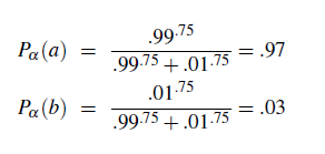
Then, given a positive pair and the $k$ negative pairs, our loss function to minimize would be

\[L_{CE} = -\log{\left[ P(+|w,c_{pos}) \cdot \prod_{i=1}^k P(- |w,c_{neg})\right]} = - \left[ \log \sigma(c_{pos} \cdot w) + \sum_{i=1}^k \log \sigma(-c_{neg} \cdot w) \right]\]

which we want to minimize by updating $\vec{w} \in W$ for the target word and $\vec{c} \in C$ for the context word.

Therefore, we need to take the derivatives:

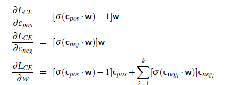
Then the update equations

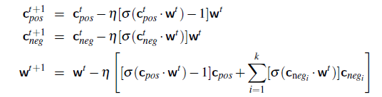
So graphically, we are doing:

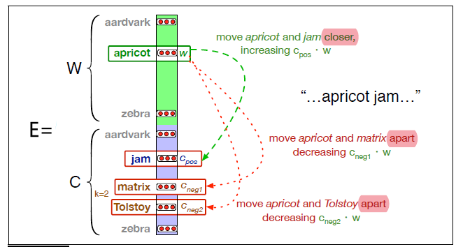
notice that we update target word embedding in $W$ but context words in $C$.

Then that is it! You now have leant two separate embeddings for each word $i$:

$\vec{w}_i = W[i]$ is the embedding target embedding for word $i$
$\vec{c}_i = C[i]$ is the embedding context embedding for word $i$

(then it is common to either just add them together as $\vec{e}_i = \vec{w}_i+\vec{c}_i$ as the embedding for word $i$, or just take $\vec{e}_i = \vec{w}_i$.)

CBOW Embedding

Essentially the reverse of Skip-Gram embedding

Intuition:

Given $2L$ context words, we need to predict the missing target word $w_t$. (we should be able to recover meaning from neighbors!)

then, while we train our model to do it, we can learn the context embedding $W,W’$ similar to the skip-gram model

hints at the idea that words physically close = words in same context is related to words being similar

Skip Gram	CBoW

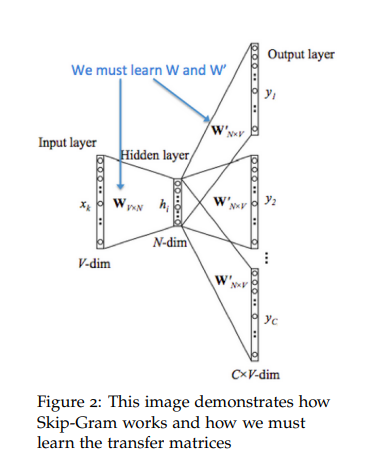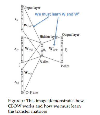where now, our idea becomes:

given our hot vectors for context words $x_{t-L},…,x_{t=1},x_{t+1}, …, x_{t+L}$
get the embedding for contexts $e_{t-L} = W^T x_{t-L}$, and etc for all the $2L$ vectors
take an average of the $2L$ embedded vectors:
\[h_t = \frac{1}{2L}(e_{t-L}+ ... + e_{t-1} + e_{t+1}+...+e_{t+L})\]
generates the output $z=W’^Th_t$
convert the output score to probability $\hat{y} = \text{Softmax}(z)$

Then, since the correct label we already know, let it be $y$. Then the loss is again cross entropy for each sample:

\[H(\hat{y},y) = -\sum_{i=1}^{|V|}y_i \log(\hat{y}_i)\]

where:

$\hat{y},y$ essentially represents probability distributions, and the above is loss for a single sample

Once done, $W,W’$ would be the embedding matrix for words and context words again.

Other Embeddings

Some problem with SGNS Embedding (Word2Vec) is:

what if we want to know the embedding of an unknown word (i.e. unseen in the training corpus)?
sparsity: in languages with rich morphology, where some of the many forms for each noun and verb may only occur rarely

There are many other kinds of word embeddings that could deal with those problems. Here we briefly cover two:

Fasttext: Fasttext deals with these problems by using subword models, representing each word as itself plus a bag of constituent n-grams, with special boundary symbols < and > added to each word

For example, with $n = 3$ the word where would be represented by the sequence <where> plus the character n-grams:
\[\text{<wh, whe, her, ere, re>}\]
then a skipgram embedding is learned for each constituent n-gram, and the word where is represented by the sum of all of the embeddings of its constituent n-grams. Therefore, Unknown words can then be presented only by the sum of the constituent n-grams!
GloVe: GloVe model is based on capturing global corpus statistics. GloVe is based on ratios of probabilities from the word-word cooccurrence matrix, combining the intuitions of count-based models like PPMI while also capturing the linear structures used by methods like word2vec.
and many more

Properties of Embedding

The embeddings learnt from machine learning related methods have the advantage of pair-wise similarity as well:

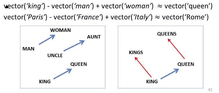
Sequence Labeling for POS and Named Entities

Parts of speech (also known as POS) and named entities are useful clues to sentence structure and meaning.

Knowing whether a word is a noun or a verb tells us about likely neighboring words (nouns in English are preceded by determiners and adjectives, verbs by nouns) and syntactic structure (verbs have dependency links to nouns), making part-of-speech tagging a key aspect of parsing
Knowing if a named entity like Washington is a name of a person, a place, or a university is important to many natural language processing tasks like question answering, stance detection, or information extraction:

Information Extraction Semantic Role Labeling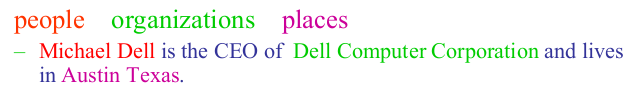

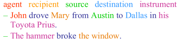
In this section, we will also introduce the

task of part-of-speech tagging, taking a sequence of words and assigning each word a part of speech like NOUN or VERB
task of named entity recognition (NER), assigning words or phrases tags like PERSON, LOCATION, or ORGANIZATION

In general

Such tasks in which we assign, to each word $x_i$ in an input word sequence, a label $y_i$, so that the output sequence $Y$ has the same length as the input sequence $X$ are called sequence labeling tasks.

This section covers models including:

generative: the Hidden Markov Model (HMM)
discriminative: Conditional Random Field (CRF), and using NN/Transformers
- ML based methods today outperform HMM

English POS

Until now we have been using part-of-speech terms like noun and verb rather freely. In this section we give more complete definitions.

In general, Part of Speech falls into two categories: open class and closed class.

Closed classes are those with relatively fixed membership, such as prepositions—new prepositions are rarely coined.

Open classes have new words within the class continually being created or borrowed.

e.g. nouns have new nouns and verbs like iPhone or to fax

Four major open classes occur in the languages of the world: nouns (including proper nouns), verbs, adjectives, and adverbs, as well as the smaller open class of interjections. English has all five, although not every language does

Now, there are also many POS tags used today. Two common ones are:

Universal Dependencies POS Tags	Penn Treebank POS Tags

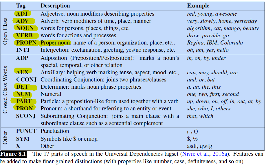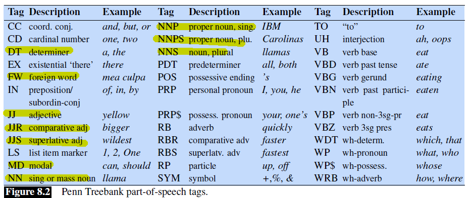where you will see some small subdivisions such as:

Common nouns include concrete terms like cat and mango, abstractions like algorithm, verb-like terms like pacing
- Many languages, including English, divide common nouns into count nouns and mass noun mass nouns.
- Count nouns can occur in the singular and plural (goat/goats, relationship/relationships) and can be counted (one goat, two goats).
- Mass nouns are used when something is conceptualized as a homogeneous group. So snow, salt, and communism are not counted
Proper nouns, like Regina, Colorado, and IBM, are names of specific persons or entities
Adverbs can also be subdivided:
- Directional adverbs or locative adverbs (home, here, downhill) specify the direction or location of some action;
- degree adverbs (extremely, very**, somewhat) specify the extent of some action, process, or manner property
etc.

Thrax’s set of eight parts of speech (results from liguistics) is the stem of many part of speech system today

noun, verb, pronoun, preposition, adverb, conjunction, participle, and article

An example of tagging would include (blue tagged with universal, red tagged with Penn Treebank):

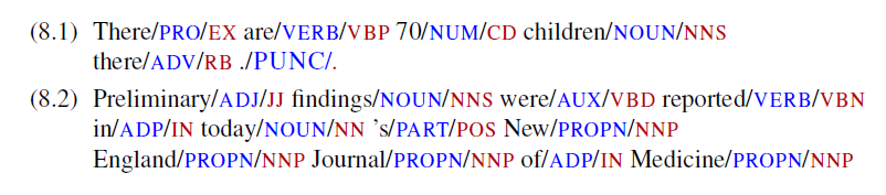
POS Tagging

Part-of-speech tagging is the process of assigning a part-of-speech tag $y_i$ to each word $x_i$ in tagging a text.

Recall

POS tagging would be useful for subsequent syntactic parsing and word sense disambiguation (i.e. knowing the correct meaning of the word in different contexts).

Tagging is a disambiguation task, because words are ambiguous—have more than one possible part-of-speech:

book can be a verb (book that flight) or a noun (hand me that book).

The goal of POS-tagging is to resolve these ambiguities, choosing the proper tag for the context

It turns out that the accuracy of part-of-speech tagging algorithms (the percentage of test set tags that match human gold labels) is extremely high.

One study found accuracies over 97% across 15 languages from the Universal Dependency (UD) treebank (Wu and Dredze, 2019).
Accuracies on various English treebanks are also 97% (no matter the algorithm; HMMs, CRFs, BERT perform similarly

But sometimes, it is the 3% that matters. But anyway here we want to know how it is done.

First, let us take a look at the task. In general:

most word types (85-86%) are unambiguous (Janet is always NNP, hesitantly is always RB)
ambiguous words, though accounting for only 14-15% of the vocabulary, are very common
- 55-67% of word tokens in running text are ambiguous

For instance, the word back can have 6 different POS in different contexts:

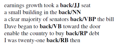
Nonetheless, many words are easy to disambiguate, because their different tags aren’t equally likely. For example, a can be a determiner or the letter a, but the determiner sense is much more likely.

Therefore, a baseline for POS tagging would be:

Most Frequent Class Baseline: given an ambiguous word (i.e. can have many tags), always assign it the tag which is most frequent in the training corpus.

this algorithm actually already have 92% accuracy

Some techniques applied today to beat the baseline include:

Rule-Based: Human crafted rules based on lexical and other linguistic knowledge.

e.g. token after a verb will be a noun

Learning-Based: Trained on human annotated corpora like the Penn Treebank.

Statistical models: Hidden Markov Model (HMM), Maximum Entropy Markov Model (MEMM), Conditional Random Field (CRF)
Rule learning: Transformation Based Learning (TBL)
Neural networks: Recurrent networks like Long Short Term Memory (LSTMs)

Note

Preprocessing, tokenization (e.g. we don’t tag punctuations) is assumed to have taken place before inputting to POS algorithms. This stage should separates and/or disambiguates punctuation, including detecting sentence boundaries.

Problems with Sequence Labeling

Some tasks that is faced with sequence labeling in general:

Not easy to integrate information from category of tokens on both sides.
- potential solution: bidirectional connections
Difficult to propagate uncertainty between decisions and “collectively” determine the most likely joint assignment of categories to all of the tokens in a sequence.
- potential solution: beam search in GNN, or probabilistic sequence models such as HMM

Tagging with HMM

Summary

An HMM is a probabilistic sequence model: given a sequence of units (words, letters, morphemes, sentences, whatever), it computes a probability distribution over possible sequences of labels and chooses the best label sequence.

Essentially it is a model based on finite state machine.

Markov Chain

A Markov chain makes a very strong assumption that if we want to predict the future in the sequence, all that matters is the current state.

Consider a sequence of state variables $q_1, …, q_i$:

\[\text{Markov Assumption}: P(q_i=a|q_1,...,q_{i-1}) = p(q_i=a|q_{i-1})\]

(basically the assumption used in bigram models)

It is then common to represent the states and probabilities as a directed graph:

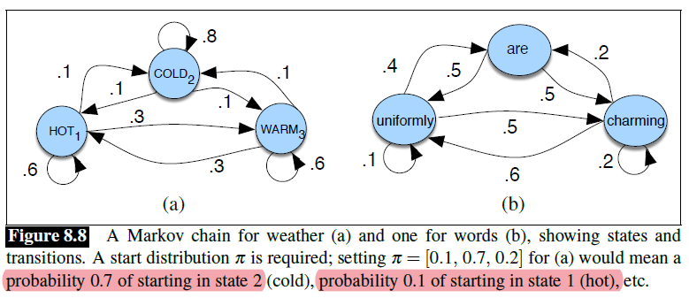
where:

The states are represented as nodes in the graph, and the transitions, with their probabilities, as edges.
A start distribution $\pi$ is required; setting $\pi = [0.1; 0.7; 0.2]$ for (a) would mean a probability $0.7$ of starting in state 2 (cold), probability $0.1$ of starting in state 1 (hot), etc.
Figure 8.8b shows a Markov chain for assigning a probability to a sequence of words $w_1,…,w_t$
- e.g. sequence hot hot hot would have a probability of $0.1 \times 0.6 \times 0.6$
- therefore, a Markov chain is useful when we need to compute a probability for a sequence of observable events

Therefore, key components in a Markov Chain include:

$Q=q_1,…,q_N$ being a set of $N$ states

$A=a_{11},a_{12},…,a_{NN}$ being a transition probability matrix $A$

each element $a_{ij}$ means probability of moving from state $i$ to state $j$

$\sum_{j=1}^Na_{ij}=1,\forall i$ so that the total probability of transitioning from state $i$ sums up to $1$

$\pi = \pi_1, …, \pi_N$ being an initial probability distribution over states.

$\pi_i$ is the probability that the Markov chain will start in state $i$.

Hidden Markov Model

The reason why we now want to consider hidden Markova model is that in reality, our observation are not states $q_i$. In fact, we observe words ($o_i$), but we will be interested in the sequence of states $q_i$ that most likely generated the sequence of words/observations.

then, essentially each state $q_i$ will be associated with a tag, then we would output a sequence of tags and our job is done
our goal would be to do:
\[\hat{t}_{1:n} = \arg\max_{t_1,...,t_n} P(t_1,...,t_n|w_1,...,w_n)\]
then we need to find away to calculate this.

Some components of hidden Markova model include:

Therefore, key components in a Hidden Markov Chain include:

$Q=q_1,…,q_N$ being a set of $N$ states

this will correspond to tags $t_i$ we need

$A=a_{11},a_{12},…,a_{NN}$ being a transition probability matrix $A$

$O=o_1,o_2,…o_T$: a sequence of $T$ observations

this will correspond to the word drawn from our vocabulary

$B=b_i(o_t)$: emission probabilities, each expressing the probability of an observation $o_t$ being generated from a state $q_i$

essentially, from a tag $t_i$, what is the probability a word $w_t$ will be generated

$\pi = \pi_1, …, \pi_N$ being an initial probability distribution over states.

$\pi_i$ is the probability that the Markov chain will start in state $i$.

(alternatively, you can also setup $q_0$ being the fixed start state, which has probabilities to other states being the $\pi$ specified above.)

First, we talk about how to construct a HMM graph and their values from some given tagged training corpus.

the transition $a_{ij}$ signifies the transition probability:
\[a_{ij}\to P(t_i |t_{i-1}) = \frac{\text{Count}(t_{i-1},t_i)}{\text{Count}(t_i)}\]
for instance, in WSJ corpus MD occurs 13124 times of which it is followed by VB 10471, for an MLE estimate then gives:
\[P(VB|MD) = \frac{10471}{13124}=0.8\]
the emission probability $b_i(o_t)$ represent the probability, given a tag (say MD), that it will be associated with a given word (say will).
\[b_i(o_t) \to P(w_i|t_i) = \frac{\text{Count}(t_{i},w_i)}{\text{Count}(t_i)}\]
For instance, of the 13124 occurrences of MD in the WSJ corpus, it is associated with will 4046 times:
\[P(will|MD) = \frac{4046}{13124} = 0.31\]

Together, we have essentially two probabilities $A,B$ to look at. Graphically:

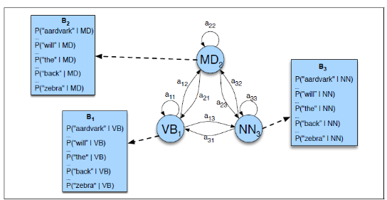
where:

the $A$ probability are the $a_{ij}\to P(t_i \vert t_{i-1})$, and the $B$ probability $P(w_i\vert t_i)$
therefore, the total number of parameters with $\lambda = {A,B}$
you might want to do smoothing techniques here as well, as you are doing counts
so essentially the hidden state $q_i=t_i$ is what we are interested in, and we want to find out the best sequence of hidden state, hence tagging, when given a sequence of observations

Formalizing this mathematically, given an observation of $n$ words:

\[\hat{t}_{1:n} = \arg\max_{t_1,...,t_n} P(t_1,...,t_n|w_1,...,w_n)\]

Then, we can simplify this by:

\[\begin{align*} \hat{t}_{1:n} &= \arg\max_{t_1,...,t_n} P(t_1,...,t_n|w_1,...,w_n)\\ &= \arg\max_{t_1,...,t_n} P(w_1,...,w_n|t_1,...,t_n)P(t_1,...,t_n)\\ &\approx \arg\max_{t_1,...,t_n} \prod_{i=1}^nP(w_i|t_i) P(t_1,...,t_n)\\ &\approx \arg\max_{t_1,...,t_n} \prod_{i=1}^n P(w_i|t_i) \prod_{j=1}^n P(t_j|t_{j-1})\\ &= \arg\max_{t_1,...,t_n} \prod_{i=1}^n P(w_i|t_i) P(t_i|t_{i-1})\\ \end{align*}\]

where:

the third equality assumed independence of neighboring words and tags
\[P(t_1,...,t_n|w_1,...,w_n) \approx \prod_{i=1}^nP(w_i|t_i)\]
the fourth equality assumed bigram for tags
\[P(t_1,...,t_n) \approx \prod_{i=1}^n P(t_i|t_{i-1})\]
the second last equality is not a nested product, hence we can simply rewrite it as a single product
now, notice that $P(w_i\vert t_i)$ and $P(t_i\vert t_{i-1})$ are known probabilities (emission and transition). So we can actually compute this task!

Before we talk about an algorithm that can solve this optimization problem, let us talk about the advantage of the this model as a generative model.

For Example: HMM Generation

Using this model, we can also generate a sequence of $T$ observations (i.e. words)

Start from some initial state $q_0$, specified by the $\pi$ distribution
For $t=1…T$
1. transit to another state $q_{t}$ from $q_{t-1}$ based on transition distribution $a_{ij}$
2. pick an observation $o_t$ (i.e. pick a word) based on the emission distribution $b_i(o_t)$

Additionally, this model can also perform the following tasks:

Observation Likelihood: To classify and order sequences.
- provide a probability score for a given sequence
- simply traverse the states and compute the probability
For example, given two sequences $O_1={o_1^1,o_2^1,…,o_n^1},O_2={o_1^2,o_2^2,…,o_n^2}$

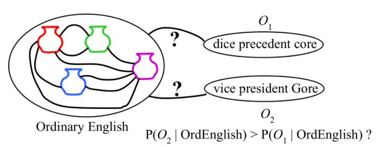
our HMM model could emit the probaility for each of them, and we can take the highest as our prediction. (similar to bigram, but more robust as we are also having syntax information)
Most likely state sequence (Decoding): To tag each token in a sequence with a label.
- the optimization task mentioned before
  \[\hat{t}_{1:n} = \arg\max_{t_1,...,t_n} P(t_1,...,t_n|w_1,...,w_n)\]
essentially spit out a sequence of hidden states (in this case, tags)

Observation Likelihood

Our first problem is to compute the likelihood of a particular observation sequence $O={o_1,…,o_n}$

Computing Likelihood: Given an HMM $\lambda = (A,B)$, i.e. the probabilities, and an observation sequence $O$, determine the likelihood $P(O\vert \lambda) \equiv P_\lambda(O)$.

this can then be used for classifying which sequence has a higher likelihood, for instance

Recall

For Markov Chain/Bigram model, we would simply say:

\[P(O|\lambda)=P_\lambda(O) = \prod_{i=1}^N P(o_i|o_{i-1})\]

however, in a HMM, emitting $o_i$ means we need to first know $q_i$, which we don’t know.

i.e. we don’t know the hidden sequence that generates the sequence $O$

To make the idea more concrete, consider the following HMM that computes how many ice-cream I will eat on each day, given a sequence of days:

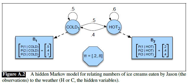
where:

the number of ice-cream I eat is the observed event $o_i$
but the number of ice-cream I eat depends on the hidden state $q_i$, which is the weather on a given day

Suppose we are given the observed sequence $O={o_1=3,o_2=1,o_3=3}$. The question is: what is the probability of this happening, i.e. $P_\lambda(O)$?

Since we only know $P(o_i\vert q_i)$, i.e. $P(1 \vert \text{hot})=0.2$, we do know the following:

\[P(O|Q) = P(o_1,...,o_T|q_1,...,q_t) = \prod_{i=1}^T P(o_i | q_i)\]

which is true due to markov’s assumption.

e.g. $P(3,1,3\vert \text{ hot,hot,cold}) = P(3\vert \text{hot})P(1\vert \text{hot})P(3\vert \text{cold})$

Then, we know that:

\[P(O) = \sum_Q P(O|Q)P(Q)\]

where $\sum_Q$ means summing over all possible sequences.

Therefore, notice that we now only need $P(Q)$:

\[P(Q)=P(q_1,...,q_t) = \prod_{i=1}^T P(q_i|q_{i-1})\]

Therefore, combining we get the probability of observing a sequence $O={o_1,…,o_T}$

\[P(O)=P(o_1,...,o_t) = \sum_Q P(O|Q)P(Q) =\sum_Q \left( \prod_{i=1}^T P(o_i | q_i)P(q_i|q_{i-1}) \right)\]

summing over all possible sequences $Q={q_1,…,q_T}$

for example, in the ice-cream case, we would have $2^3=8$ possible cases for our observation being length $T=3$:
\[P(3,1,3) = P(3,1,3, \text{cold, cold, cold})+P(3,1,3, \text{cold, cold, hot})+...\]
for an HMM with $N$ hidden states and an observation sequence of $T$ observations, there are $N^T$ possible observations. In practice this would be a pain to compute directly, so we have the following forward algorithm.

Forward Algorithm is a kind of dynamic programming algorithm that can compltet this task in $O(N^2T)$ by implicitly folding each of these paths into a single forward trellis

Essentially, realize that computing $P(3,1\vert \text{ hot hot})$ and $P(3,1\vert \text{ hot cold})$ results in:

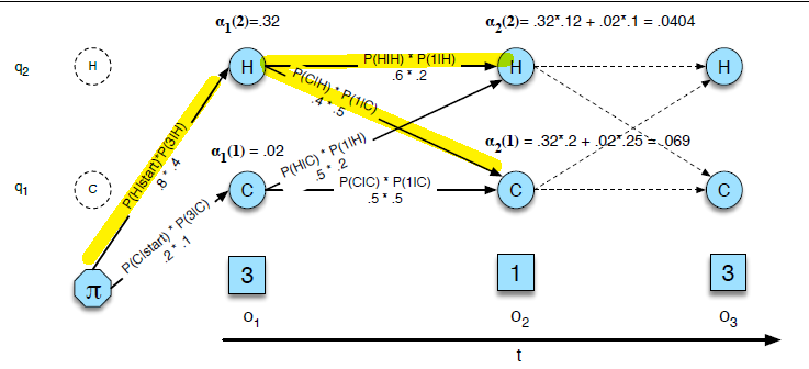
where the key idea is to realize that they are sharing the same path:

therefore, the key insight to speed up computation is to realize that each cell at $t=2$ only depends on the previous cells $t=1$.

Let us represent:

$\alpha_{t}(j)$ being the probability of being in state $j$ after the first $t$ observations = emitting $o_t$ at $q_t=j$ This means that:
\[\alpha_{t}(j) = P_\lambda(o_1,...,o_t,q_t = j)\]
e.g. probability of being in $q_2 = \text{hot}$ after seeing the first $1$ observation $o_1=3$. Hence graphically:
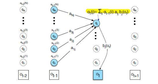
Therefore, the we can compute it by:
\[\alpha_t(j) = \sum_{i=1}^N \underbrace{\alpha_{t-1}(i)a_{ij}}_{\text{get to state $q_j$}}\quad \underbrace{b_j(o_t)}_{\text{emit $o_t$ at $q_t$}}\]
whic should be pretty clear form the graph, so that:
- $\alpha_{t-1}(i)$ is previous forward path probability from the previous time step
- $a_{ij}$ is the transitioni probability to state $q_t=j$, i.e. the current focus
- $b_j(o_t)$ is the state observation likelihood/emission probability to emit $o_t$ when you are at state $q_t=j$
  - i.e. emitting $P(o_t=3\vert q_t = \text{hot})$

For Example. Given the following HMM, and $O={3,1,3}$

what would be $\alpha_2(2)$?

Solution: Essentially this means $t=2,j=2$, that we are emitting $o_2=1$ at state $q_t=2=\text{hot}$. Hence:

\[\alpha_2(a)=\alpha_{1}(1)\cdot P(H|C)\cdot P(1|H) + \alpha_{1}(2)\cdot P(H|H)\cdot P(1|H)\]

The answer is essentially

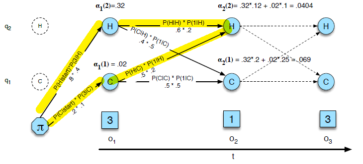
With that, the algorithm basically does:

Given a sequence of observation $o_1,…,o_t$

Initialization:
\[\alpha_1(j)=P(o_1,q_1=j) = \pi_j b_j(o_1),\quad 1 \le j \le N\]
i.e. probability of emitting $o_1$ at each state
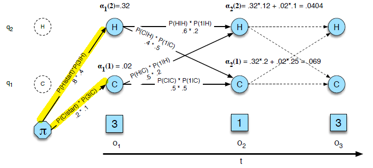
Recursion. Iterate for $t=2…T$:
\[\alpha_t(j) = \sum_{i=1}^N \alpha_{t-1}(i)a_{ij}b_j(o_t),\quad 1 \le j \le N\]
graphically:

$t=2$ $t=3$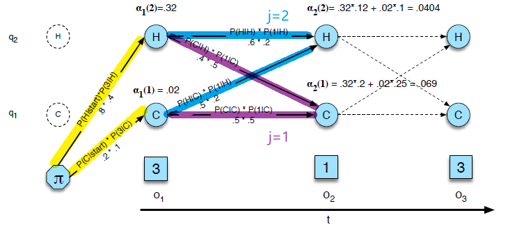
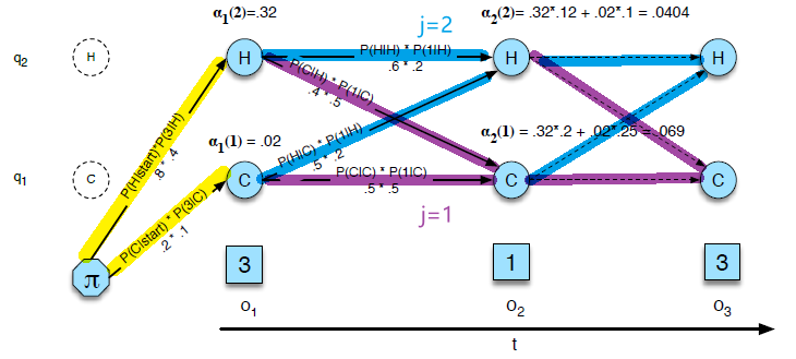
Termination: Sum over the last cells:
\[P(O|\lambda) = \sum_{i=1}^N \alpha_T(i)\]
graphically:

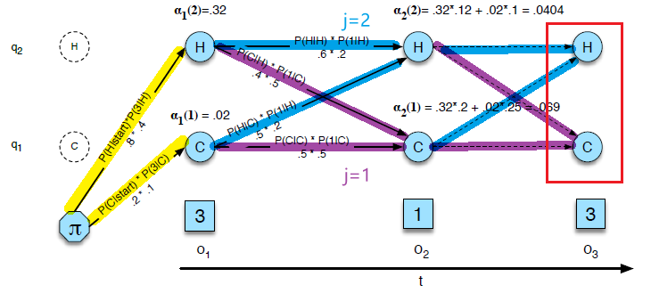
Then the actual algorithm pseudo-code:

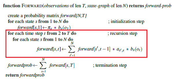
which you can see the main loops goes to $T\cdot N \cdot N$, hence we have $O(TN^2)$

Decoding: The Viterbi Algorithm

Now, we consider performing POS Tagging for a given observation $O$. This means essentially we need to compute:

\[\hat{t}_{1:n} = \arg\max_{t_1,...,t_n} P(t_1,...,t_n|w_1,...,w_n)\]

which can be generalized to the task of sequence labeling/most likely sequence

Decoding: Given as input an HMM $\lambda = (A,B)$ and a sequence of observations $O = o_1,…,o_T$ , find the most probable sequence of states $Q=q_1,...,q_T$ .

Consider again the example of number of ice-cream eaten per day:

give a sequence $3,1,3$, what is the best likely weather sequence? e.g. $P(H,H,H\vert 3,1,3)=?$
For each possible sequence, e.g. $(HHH, HHC, HCH)$, we could run the forward algorithm and compute the likelihood of the observation sequence given that hidden state sequence. This is brute force and takes an exponentially large number of state sequences.

Then, the idea is as follows:

at each time step $t$, for each state $q_t=j,1 \le j \le N$, we can store a best path that arrived there:
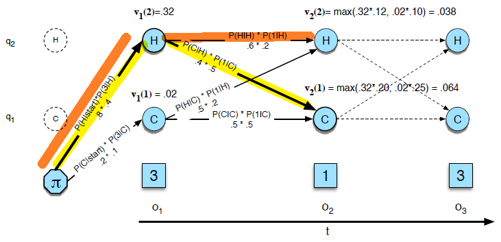
Then, once we have computed the probability and propagated to the end, we can backtrace and get the optimal path

Therefore, the viterbi algorithm essentially does:

consider at each time step $t$, we want to know:
\[v_{t}(j) = \max_{q_1,...,q_{t-1}}P_\lambda(o_1,...,o_t,q_t = j)\]
This can be computed from iterating over the previous best scores $v_{t-1}$, taking the best, and save a “checkpoint/back pointer”.
\[v_t(j) = \max_{q_1,...,q_{t-1}}\,\, \underbrace{v_{t-1}(i)a_{ij}}_{\text{get to state $q_j$}}\quad \underbrace{b_j(o_t)}_{\text{emit $o_t$ at $q_t$}}\]
note that
- the only difference of this with the forward algorithm is that it was 1. taking the sum; 2. no need to store a back pointer/checkpoint
- The reason is that while the forward algorithm needs to produce an observation likelihood, the Viterbi algorithm must produce a probability and also the most likely state sequence.
When we have the back pointers, it look like:

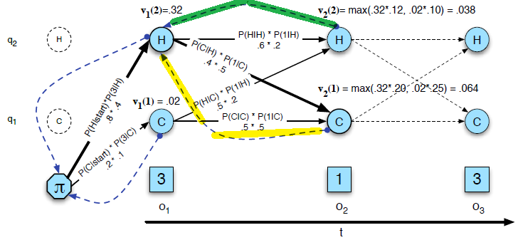
which we only need to backtrack one step per node.
Then, all yuo need to do is to backtracing the best path to the beginning using the saved back pointers

So the algorithm looks like Given a sequence of observation $o_1,…,o_t$

Initialization:
\[\begin{align*} v_1(j) &= \pi_j b_j(o_1),&1 \le j \le N\\ bt_1(j) &= 0, & 1 \le j \le N \end{align*}\]
where $bt_1(j)$ means the back pointer of state $q_1=j$ is $q_0$,
Recursion. Iterate for $t=2…T$:
\[\begin{align*} \alpha_t(j) &= \max_{i=1...N}\,\,v_{t-1}(i)a_{ij}b_j(o_t),\quad 1 \le j \le N\\ bt_t(j)& = \arg\max_{i=1...N}\,\, v_{t-1}(i)a_{ij}b_j(o_t),\quad 1 \le j \le N \end{align*}\]
so in addition to moving forward, we are saving the best back pointer of $q_t=j$ being $q_{t-1}=i$
Termination: The best score by comparing over the last cells:
\[\begin{align*} \text{Best Score}: \quad &P^* = \max_{i=1...N} v_T(i)\\ \text{Start of Backtrace}: \quad &q_T^* = \arg\max_{i=1...N} v_T(i) \end{align*}\]

Hence the algorithm pseudo-code looks like:

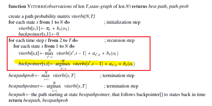
which is again $O(N^2T)$ as it is almost the same as the forward algorithm.

Unsupervised HMM

Recall that

for supervised learning, there is a problem that we may not have those tagged dataset/becomes useless if we want to do it in an different language
it turns out that we can train a HMM even in an unsupervised setting.

Given an observation sequence, $O={o_1, o_2, …, 0n}$, what set of parameters, $λ=(A,B)$, for a given model maximizes the probability that this data was generated from this model $P(O\vert \lambda)=P\lambda(O)$?

but now, data ara unlabelled so we cannot use counts.

Reminder: EM algorithm

The idea of EM algorithm is basically as follows:

computing an initial estimate for the probabilities
using those estimates to computing a better estimate
repeat

In more details:

Initialize the parameters arbitrarily
Given the current setting of parameters find the best (soft) assignment of data samples to the clusters (Expectation-step)
- this soft partition basically means, we assign proportion of the data to each Gaussian mountain
  
  e.g. if we have four mountains represented by X in the below figure, each has a $P_i$ estimate of the data $\vec{x}$ in the circle,
  
  then, e.g. mountain 3 will get the proportion
  \[\frac{P_1}{P_1+P_2+P_3+P_4}\]
- in the Lloyd’s Algorithm for the K-means, the idea is similar in that we assign the data point completely (hard) to the closest cluster (closest to the mean)
Update all the parameters $\theta$ with respect to the current (soft) assignment that maximizes the likelihood (Maximization-step)
- same idea as Lloyd’s algorithm
- this is now basically MLE
Repeat until no more progress is made.

An example of what it looked like:

Arbitrary Initialization	E-Step, Soft Assignment	M-Step, Optimize	After 5 Rounds	After 20 rounds
		!

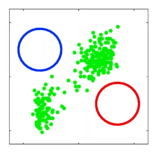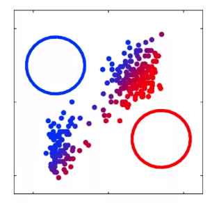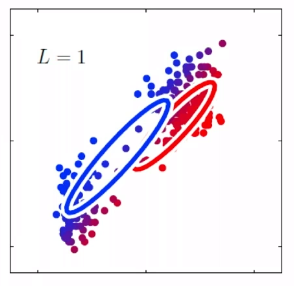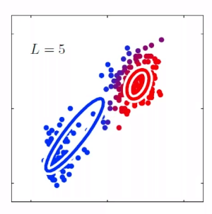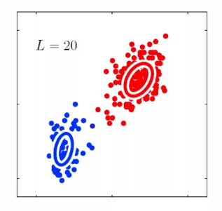The standard algorithm for HMM training is the forward-backward, or Baum Welch algorithm (Baum, 1972), a special case of the Expectation-Maximization or EM algorithm

A brief sketch of the algorithm is provided below.

Assume an HMM with $N$ states.

Randomly set its parameters $\lambda = (A,B)$
- (making sure they represent legal distributions)
Do until converge (i.e. $\lambda$ no longer changes):
- E Step: Use the forward/backward procedure to determine the probability of various possible state sequences for generating the training data
- M Step: Use these probability estimates to re-estimate values for all of the parameters $λ$

Note that in general, for EM type algorithms:

Each iteration changes the parameters in a way that is guaranteed to increase the likelihood of the data: $P(O\vert \lambda )=P_\lambda (O)$.
Converges to a local maximum.

Semi-Supervised HMM

EM Algorithm can be exploited to deal with:

a mix of labeled and unlabeled data

even purely supervised data

When you have a mix of labeled and unlabeled data.

Use supervised learning on labeled data to initialize the parameters (instead of initializing them randomly).
Essentially soft label for unlabelled data, but hard assignments for labelled data.

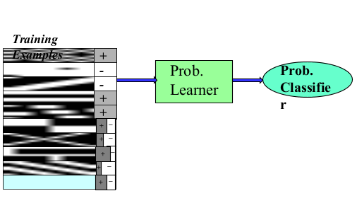
Note

Use of additional unlabeled data improves on supervised learning when amount of labeled data is very small and amount of unlabeled data is large.

otherwise, if unlabelled data is small, it could degrade performance when there is sufficient when unsupervised learning tends to create labels that are incompatible with the labelled/desired ones.

When you have supervised data and you want to use EM

Use supervised learning on labeled data to initialize the parameters (instead of initializing them randomly).
Use known labels for supervised data instead of predicting soft labels for these examples during retraining iterations.

Constituency Grammar and Parsing

Essentially we discuss how syntax/grammar works, by exploring the idea of context-free grammar which is the backbone of many formal models of the syntax of natural languages.

Syntactic constituency is the idea that groups of words can behave as single units, or constituents.

e.g. a noun phrase NP, a sequence of words surrounding at least one noun

A more specific example would be:

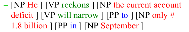
Context Free Grammar

The most widely used formal system for modeling constituent structure in English and other natural languages is the Context-Free Grammar, CFG. Essentially:

A context-free grammar consists of a set of rules or productions, each of which expresses the ways that symbols of the language can be grouped and ordered together, and a lexicon of words and symbols

Goal: The problem of mapping from a string of words to its parse tree is called syntactic parsing

Definition of Context Free Grammar:

A context-free grammar is a tuple $(N, \Sigma, R, S)$, where

$N$ is a finite set of non-terminal symbols/single variables

it is exactly because it only allow a single variable, it is context free because it only depends on that variable without context

$\Sigma$ is a set of terminal symbols/an alphabet (finite). This is disjoint from $N$.

$R$ is a finite set of rules of the form:
\[A \to w;\,\,A\in N;\,\,w\in(V\cup\Sigma)^*\]
so basically, you can have more than one variables, and each variable points to either a string or a string+another variable.

In general, for generating an non-empty language, you need to have at least one rule that points to a symbol only.

$S \in N$ is the start variable

We will use the following notation for CFG in this case:

Capital letters such as $A,B,S$ represents non-terminals
Lower-case roman letters such as $u,v,w$ are strings of terminals
$S$ is the start symbol
Lower-case letters such as $\alpha, \beta, \gamma$ are strings from $(\Sigma \cup N)^*$

Recap from CS Theory

If two string $\alpha, \gamma \in (N \cup \Sigma)^*$, and there is a rule $A \to \beta \in R$, then we can write:
\[\alpha A \gamma \Rightarrow \alpha \beta \gamma\]
which reads: $\alpha A\gamma$ yields $\alpha \beta \gamma$.

If two string $\alpha_1, \alpha_m \in (N \cup \Sigma)^$, we say that $\alpha_1 \Rightarrow^* \alpha_m$ if some $\alpha_2, …,\alpha_{m-1} \in (N \cup \Sigma)^$ we have:
\[\alpha_1 \Rightarrow \alpha_2 \Rightarrow \alpha_3 \Rightarrow ... \Rightarrow \alpha_m\]
where:

$\alpha_1,\alpha_2, …,\alpha_m$ are just strings that you can reach from its previous string.

This basically means that $\alpha_1$ generates to $\alpha_m$ if there is an arbitrary number of step that can make we start with $u$ and end in $v$.

e.g. $S \Rightarrow^* 0011$ in the example above

Notice that:

when you specify rules, you use $\to$, when you show derivations, you use $\Rightarrow$

And correspondingly:

Context Free Language Def:

A language $L$ is a context-free language if there exists a context free grammar $G$ such that $L(G)=L$.

i.e. set of strings composed of terminal symbols that can be derived from the designated start symbol $S$

Syntax and CFG

Now, we can illustrate some examples how this relates to syntax in reality.

terminal $\Sigma$: The symbols that correspond to words in the language (“the”, “nightclub”) are called terminal symbol
nonterminal $N$: The symbols that express abstractions over these terminals are called non-terminals
start symbol $S$: can be thought of as a sentence node

For instance, the ATIS English corpus provides the following CFG definitions for English

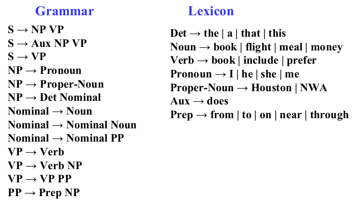
where we can see all rules/productions that are possible, and that:

PP is a prepositional phrase
notice that the terminals cannot be on the LHS of the rule, whereas non-terminals such as VP can be on both LHS and RHS of a grammar rule.
Lexicons are basically rules that generate terminals/words

And we can use CFG in two ways:

generating sentences/derivation.
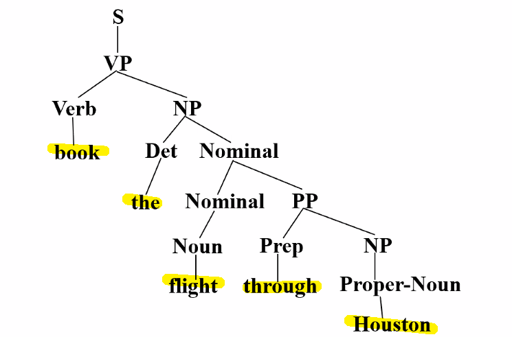
as a device for assigning a structure to a given sentence (i.e. output a parse tree)

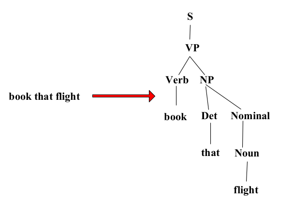
where sometimes you are asked to
- return a parse tree for the string
- or return all possible parse trees for the string

Both can be represented as a parse tree. For instance:

Parse Tree	Bracketed Notation

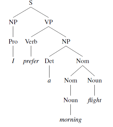Grammar Equivalence and Normal Form

In fact, it is possible to have two distinct context-free grammars generate the same language.

Two grammars are strongly equivalent if they generate the same set of strings and if they assign the same phrase structure to each sentence (allowing merely for renaming of the non-terminal symbols).

Two grammars are weakly equivalent if they generate the same set of strings but do not assign the same phrase structure to each sentence.

Additionally, a single sentence can have multiple parse trees, which means ambiguity in structure, and this will be covered in a another section.

It is sometimes useful to have a normal form for grammars, in which each of the productions takes a particular form. For example, a common context-free grammar form used is Chomsky normal form (CNF) (Chomsky, 1963)

Chomsky normal form (CNF)

A CFG is in Chomsky normal form it is

$\epsilon$-free, i.e. no empty string

each production is either of the form $A\to BC$ or $A\to a$. That is, the right-hand side of each rule either has two non-terminal symbols or one terminal symbol

Therefore, CNF parse trees are binary branching.

For instance, you can convert $A \to BCD$ to CNF by:

\[\begin{cases} A \to BX\\ X \to CD \end{cases}\]

where you added a non-terminal $X$.

Partial Parsing

Before going right into finding a parse tree given a sentence, we first consider some other simpler yet related task.

Many language processing tasks do not require complex, complete parse trees for all inputs. For these tasks, a partial parse, or shallow parse, of input sentences may be sufficient.
one kind of partial parsing is chunking

Chunking is a process of extracting flat phrases from unstructured text.

e.g. identifying phrases such as “South Africa” as a single phrase instead of ‘South’ and ‘Africa’ as two tokens

there is no hierarchical structure in the result, hence less informative than tree parsing

Since chunked texts lack a hierarchical structure, a simple bracketing notation is sufficient to denote the location and the type of the chunks in a given example:

\[\text{$[_{NP}$ The morning flight] $[_{PP}$ from] $[_{NP}$ Denver] $[_{VP}$ has arrived.]}\]

this makes clear that chunking invovles two tasks:

segmenting (finding the non-overlapping extents of the chunks)
labeling (assigning the correct tag to the discovered chunks).
in different applications, some input words may not be part of any chunk. For example, if you consider base $NP$ chunking:
\[\text{$[_{NP}$ The morning flight] from $[_{NP}$ Denver] has arrived.}\]

In most approaches, base phrases include the headword of the phrase, along with any pre-head material within the constituent, while crucially excluding any post-head material.

For instance:
\[\text{$[_{NP}$ a flight] $[_{PP}$ from] $[_{NP}$ Indianapolis]$[_{PP}$ to]$[_{NP}$ Houston]}\]
has:

$[_{NP} \text{ a flight}]$ for flight being the headwords of the NP, and a being the pre-head.

Chunking Algorithms

Chunking is generally done via supervised learning, training a BIO sequence labeler. In BIO tagging, we have

a tag for the beginning (B)
inside (I) of each chunk type,
tokens outside (O) any chunk

For instance:

All	Base NP

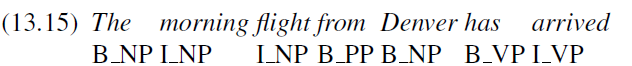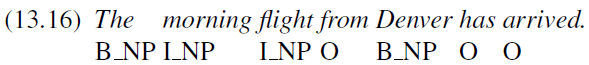where notice that:

for all base phrase, we don’t need O tags
for base NP only, we need O tag to show the boundaries

Then, given a training set, any sequence model can be used to chunk: CRF, RNN, Transformer, etc

To evaluate our performance, we are strict in that:

\[\begin{align*} \text{Precision}&=P=\frac{\text{Number of correct chunks found}}{\text{Total number of chunks found}}\\ \text{Recall}&=R=\frac{\text{Number of correct chunks found}}{\text{Total number of chunks}} \end{align*}\]

note that if one part of the phrase is labeled as wrong, the entire chunk is wrong

Take harmonic mean to produce a single evaluation metric called F measure.:

\[F_\beta = \frac{(\beta^2 + 1)P\cdot R}{\beta^2 P + R}\]

and mostly commonly $F_1$ is used:

\[F_1 = \frac{2PR}{P+2} = \frac{1}{2[(1/P) + (1/R)]}\]

current best system for NP chunking: F1=96%
most other models also have around F1=92-94%

Brute Force Parsing

Our task of parsing a give sentence is essentially:

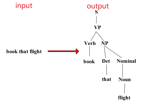
Intuition

This means we need to search space of derivations for one that derives the given string.

Top-Down Parsing: Start searching space of derivations from the start symbol.

Bottom-up Parsing: Start search space of reverse deviations from the terminal symbols in the string.

Top-Down Parsing

Essentially trial and errors, with backtracking once an error is made

if a mistake is made, backtrack one step
if no more tries are left, backtrack one step

Consider parsing the sentence $\text{book that flight}$:

Start with top and try to fit book:

Try NP -> Pronoun NP -> ProperNoun Aux Success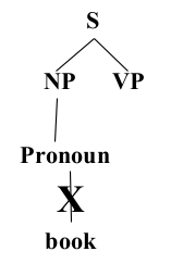

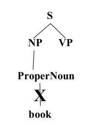
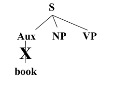
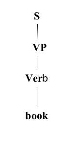
Try fitting that:

No more options/production	Backtrack One Step	Failed	Success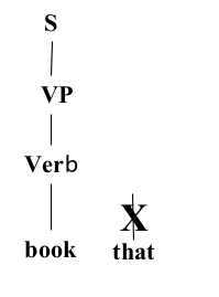

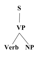
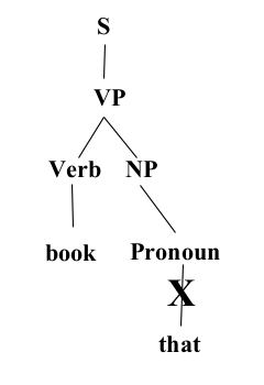
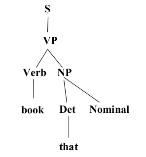
notice that you only backtracked to fix previous problems when you ran out of current options.

Finally:

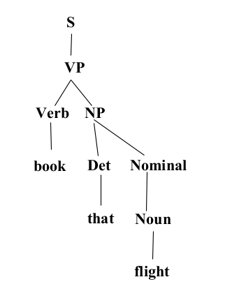
Bottom-Up Parsing

The same idea, but now you start with bottom/tokens

Start with book, and try to fit that and flight

Failed Backtrack, no more options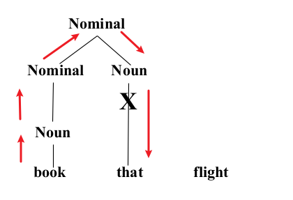
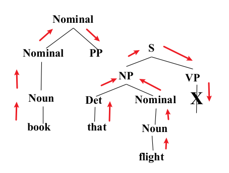
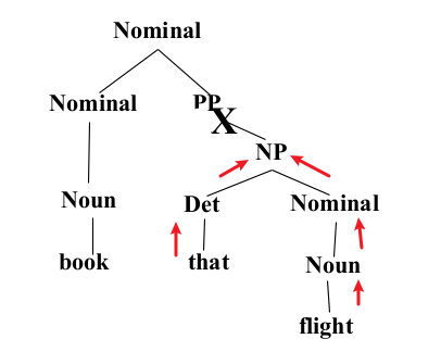
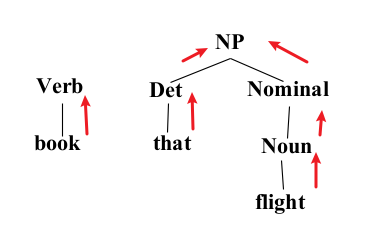
Try other options with book by backtracking this

Failed Success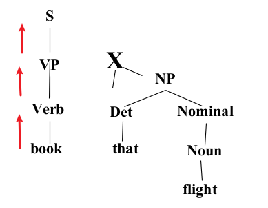

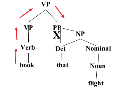
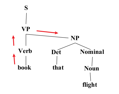
notice that we cached/saved what has been working on the right branch as we backtrack the “deepest” step one at a time

Top-down Bottom-Up Comparison

Top down never explores options that will not lead to a full parse, but can explore many options that never connect to the actual sentence.
Bottom up never explores options that do not connect to the actual sentence but can explore options that can never lead to a full parse.
Relative amounts of wasted search depend on how much the grammar branches in each direction.

Therefore, the idea is to use dynamic programming to save those wasted computations (though still $O(n^3)$ for $n$ is the length of input string)

CKY Algorithm - based on bottom-up parsing
Earley Parser - based on top-down parsing
Chart Parsers - combine top-down and bottom-up search.

CKY Algorithm

The CKY algorithm requires grammars to first be in Chomsky Normal Form (CNF).

productions must have either exactly 2 non-terminal symbols on the RHS or 1 terminal symbol (lexicon rules).

Note: converting to CNF form.

In general, we have three cases to deal with:

Rules with a single non-terminal on the right are called unit productions.

if $A \Rightarrow^* B$ by a chain of one or more unit productions and $B \to \gamma$ is a non-unit production in our grammar, then we add $A \to \gamma$ for each such rule int he grammar and discard all the intervening unit productions.

Rules with right-hand sides longer than 2 are normalized through the introduction of new non-terminals

This is simple, if you have $A \to BC\gamma$, then:
\[A \to X\gamma\\ X \to BC\]
would work.

A full example looks like:

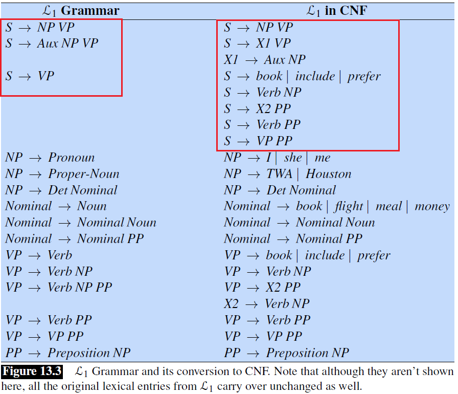
as an exercise you can try to reproduce the red highlighted parts.

CKY Recognition

The CKY algorithm can do two things/have two versions:

recognizer: ell us whether a valid parse exists for a given sentence
parser: in addition to recognizer, provide all possible parse trees

Here, we start with the simple base model of recognizer. In essence, the algorithm considers a two dimensional matrix

our index start with $0$
each cell $[i,j]$ means the set of non-terminals that represent all the constituents that span positions $i$ through $j$ of the input
since it is a CNF form, we can think of a node $[i,j]$ having branched to a node below it $[i+,j]$** and a **node left of it $[i,j-]$. This works because each non-terminal production has exactly two children.

An example of recognizing the sentence $\text{Book the flight through Houston}$ looks like:

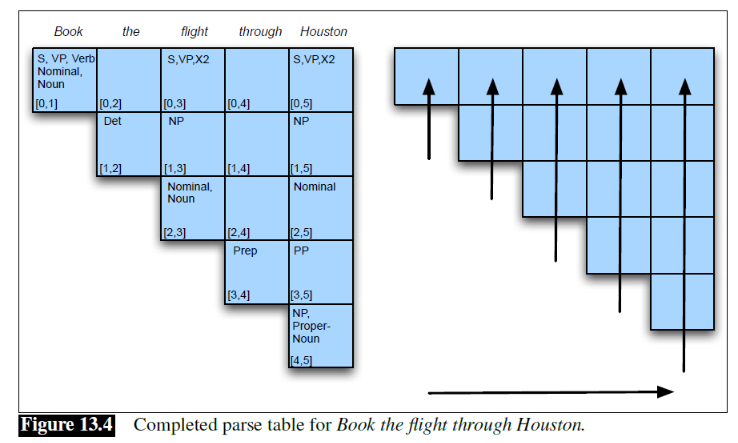
notice that:

the cell that represents the entire input resides in position $[0,n]$ in the matrix
the right figure demonstrates the order the non-terminals are filled. This order guarantees that at the point where we are filling any cell $[i, j]$, the cells containing the parts that could contribute to this entry (i.e. the cells to the left and the cells below) have already been filled.
The superdiagonal row (lowest diagonal) in the matrix contains the parts of speech for each word in the input. The subsequent diagonals above that superdiagonal contain constituents with increasing length
finally, all we need to check is if there is a $S$ in the $[0,n]$-th cell of the matrix. If there is, then there exists a valid parsing, otherwise there isn’t.

In specific, each cell $[i,j]$ is filled by considering all the following possibilities:

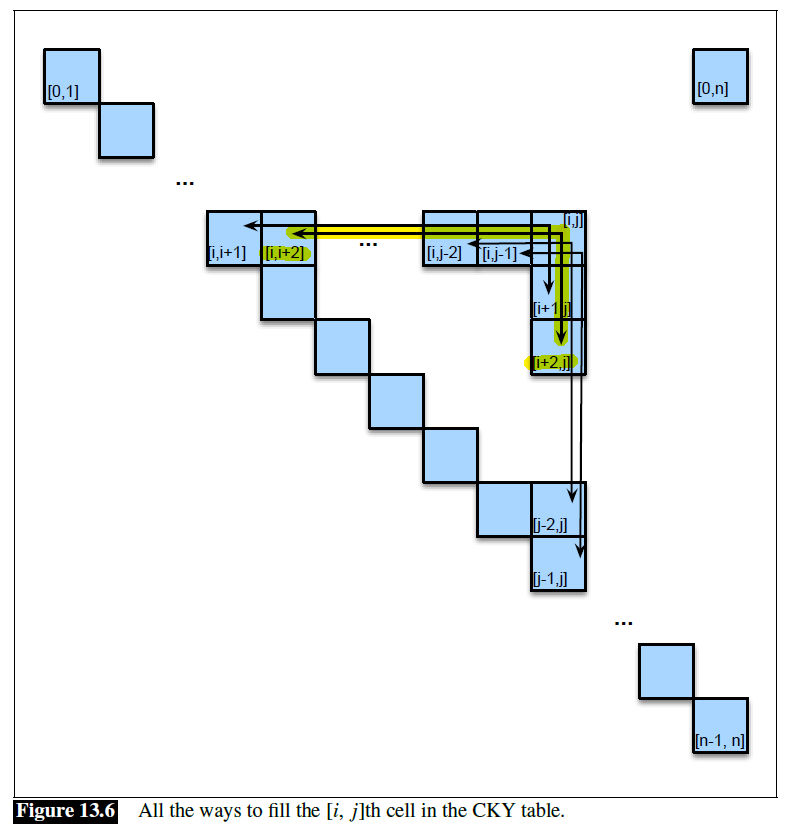
where for instance:

the cell $[i,j+2]$ and $[i+2,j]$ represents parsing for combining first 2 blocks starting from $i$, and the 3rd block to current block respectively.

Hence, the algorithm looks like:

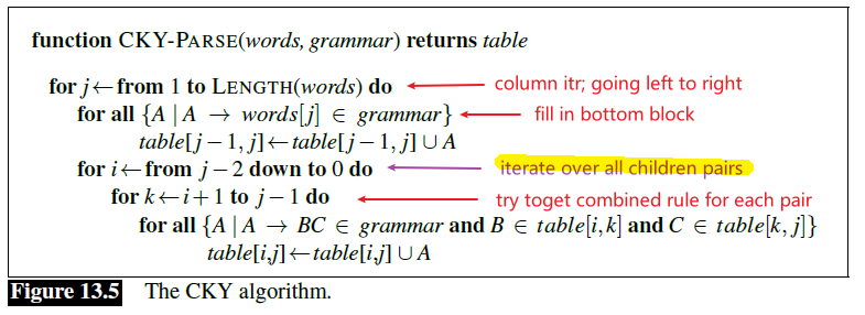
where it is important to note that the highlighted loop is essentially trying the combined pairs in the above figure (13.6).

The algorithm given in Fig. 13.5 is a recognizer, not a parser.

CKY Parser

Though the above algorithm is not a parser, it can be easily modified into a parser by doing the following:

we need to store, for each non-terminal, pointers to the table entries from which it was derived

For example:

No Match, Next Works, Save Pointer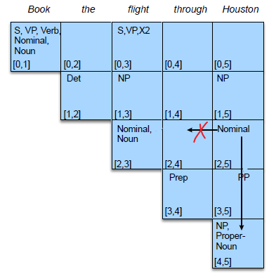
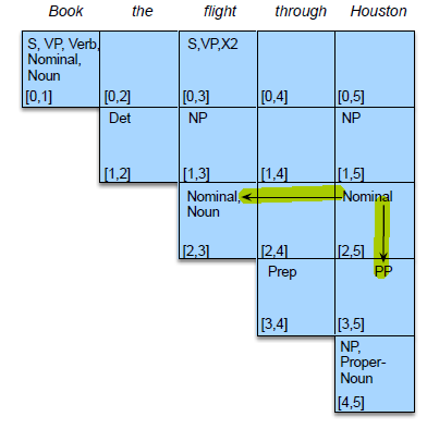
permit multiple versions of the same non-terminal to be entered into the table (e.g. we can have multiple possible parse trees)

For example:

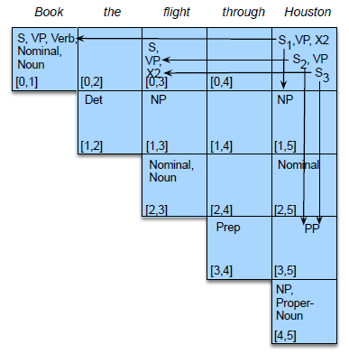
Then, returning

an arbitrary single parse consists of choosing an $S$ from cell $[0,n]$, i.e. the last cell on top right.
then recursively retrieving its component constituents from the table

would give us all possible parse trees.

The problem now is it doesn’t tell us which parse is the correct one! That is, it doesn’t disambiguate among the possible parses.

the intuition to fix this would be to use a simple neural network extension to provide scores to each parse tree

or use PCFG, i.e. each rule will have an associated probability, hence parse tree has a score/probability!

Lastly, we consider the complexity.

we need to iterate over $O(n^2)$ cells
for each cell, look at all possible splits/combinations. There are $O(n)$ of them

Hence, we have:

\[O(n^3)\]

as the time complexity.

Problems with CFG

Is CFG practical to represent rules under the language we speak?

In reality, those are not complete as there could be so many more specific grammar rules within a single language
additionally, the conversion to CNF will complicate any syntax-driven approach to semantic analysis

For Example: Word Agreement:

we need subject-verb agreement such as:
\[\text{I am cold.} \quad vs \quad \text{*I are cold}\]
both of which will be parsed by the CKY, as both am and are are verb.

To fix issues like this, we need separate production rules for each combination
- S -> NP1stPersonSing VP1stPersonSing
- S → NP2ndPersonSing VP2ndPersonSing
- NP1stPersonSing → …
- VP1stPersonSing → …
- etc
pronoun agreement:
\[\text{I gave him the book.} \quad vs \quad \text{*I gave he the book}\]
again, we need more rules that what we have to correctly deal with them.

For Example: Subcategorization

Specific verbs have specific rules for words after them. For example:

\[\text{John wants to buy a car.} \quad vs \quad \text{*John wants buy a car.}\]

Again, more specific rules are needed for different tokens, this cannot be characterized by our current CFG.

In short, even if the CKY runtime will be $O(N^3)$, it depends on having prepared the grammar, which could be exponential in size. Hence this could be a bottleneck one has to deal with.

Statistical Parsing

A PCFG is a probabilistic version of a CFG where each production has a probability. By adding a probability to production rules, one can an approach to resolving syntactic ambiguity, i.e. it produces a score for each parse tree.

Definition of Probabalistic Context Free Grammar:

A context-free grammar is a tuple $(N, \Sigma, R, S)$, where

$N$ is a finite set of non-terminal symbols/single variables

it is exactly because it only allow a single variable, it is context free because it only depends on that variable without context

$\Sigma$ is a set of terminal symbols/an alphabet (finite). This is disjoint from $N$.

$R$ is a finite set of probabalistic rules of the form:
\[A \to \beta[p],\, p\equiv p(A \to \beta |A); \quad \,A\in N;\,\,\beta \in(V\cup\Sigma)^*\]
which is probabalistic, meaning the probability of expanding to $\beta$ when given the non-terminal $A$. Therefore necessarily we need:
\[\sum_\beta p(A \to \beta| A)=1\]

$S \in N$ is the start variable

So a probabilistic context-free grammar is also defined by four parameters, with a slight augmentation to each of the rules in $R$.

For Example

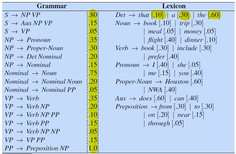
and notice that, for instance $\sum_\beta p(S \to \beta \vert S)=1$ is the first three rows of the table.

This would be useful because we can define the probability of a particular parse tree $T$ of a setnence $S$ being:

\[P(T,S)=P(T)=\prod_{i=1}^nP(\text{RHS}_i|\text{LHS}_i)\]

where each rule $i$ is being expressed as $\text{LHS}_i \to \text{RHS}_i$.

$P(T,S)=P(S\vert T)P(T)=P(T)$ since given the tree $P(S\vert T)=1$ includes all words of the sentence.
so all we need to do it to multiply probabilities of each of the rules used in the derivation, to get a score/probability of a parse tree $P(T)$!.

An example would be:

Parse Tree	Probability CFG

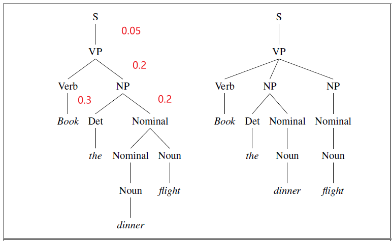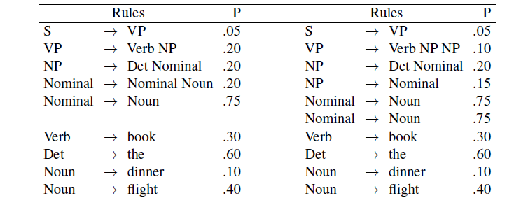And as an exercise, make sure the following is correct:

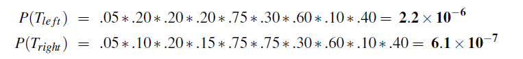
Then, with the single capability of providing a score to a parse tree, we can do:

Observation likelihood: To classify and order sentences.
Most likely derivation: To determine the most likely parse tree for a sentence.
(Finding the probability for the rules) Maximum likelihood training: To train a PCFG to fit empirical training data.

PCFG Most Likely Derivation

With the ability to assign a score to a tree $T$, we can basically do disambiguation by picking the most probable:

\[\hat{T}(S) = \arg\max_T P(T|S)=\arg\max_T P(T,S)=\arg\max_T P(T)\]

since $P(S)$ is a constant, and $P(T,S)=P(T)$. Baically we just choose the parse with highest probability.

Then, the algorithms for computing the most likely parse are simple extensions of the standard algorithms for parsing, i.e. augmenting CKY algorithm with probabilities.

Therefore, the idea is basically:

Convert the rules to CNF, so that right-hand side of each rule must expand to either two non-terminals or to a single terminal. This is non-trivial as it involves also converting probabilities while breaking into CNF.
For probabilistic CKY, it’s slightly simpler to think of the each cell in the matrix $M[i,j,A]$ as constituting a third dimension of maximum length $V$: corresponds to each non-terminal that can be placed in this cell, e.g. $A_1 \to BC$ being a cell in the third dimension, then next $A_2 \to DE$, etc.

The value of the cell is then a probability for that nonterminal/constituent (then of course many of those cells in the third dimension will have value $0$ since most rules cannot produce the constituent $S[i:j]$).
Lastly, the entire CKY algorithm is the same, except at each step we update the probability

For example:

Computation Matrix	PCFG

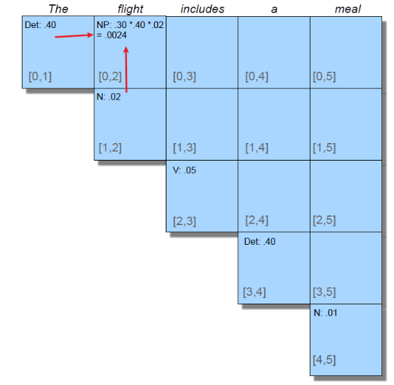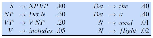And the algorithm is simply:

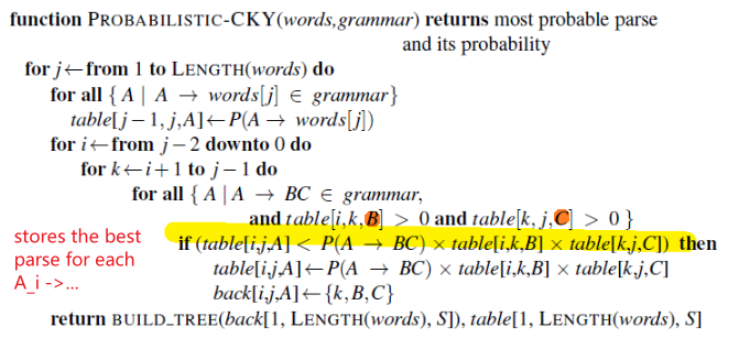
as compared to the original CKY, which is basically concatenating each rule $A_i$ at the cell $T[i,j]$.

and again, since in the end we need to spit out a tree, we also need to keep a backtrack matrix which is the last step in the innermost loop of the algorithm.

For a better visualization, at cell $T[1,4]$, the will do:

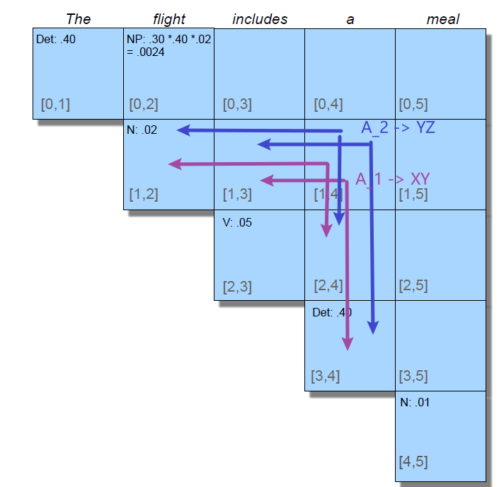
for every possible rule $A_i \to …$, and each cell $T[1,4,A_i]$ records the best arrow combination for rule $A_i$ (e.g. which of the two purple is better for rule $A_1$ is recorded at $T[1,4,A_1]$, and so on for $A_2$…)

For Example: Convert CFG Probability

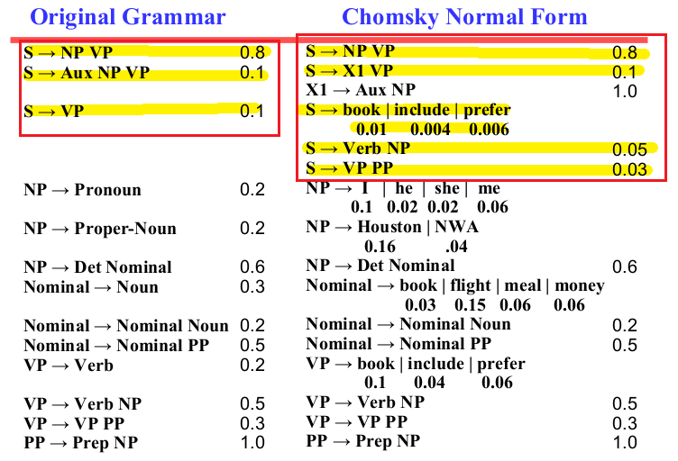
Notice how the red boxes is converted to the red boxes on the right, while the yellow highlighted part obeyed that:

\[\sum_\beta P(A\to \beta |A)=1\]

PCFG Observation Likelihood

If we can quantify the probability of a parse tree, we can also quantify the probability of a sentence. Hence we can directly assign scores to a sentence!

The probability of an ambiguous sentence is the sum of the probabilities of all the parse trees for the sentence

\[P(S) = \sum_{T} P(T,S) = \sum_T P(T)\]

Therefore, since in this case we only needs to spit out a score, we do:

for each possible rule $A_i \to XY$, we want to combine all the probability of all possible parse instead of only taking the max
do CKY while keeping the sum for each cell in the third dimension
return the sum of the third dimension on the last cell $\text{sum}_i(T[0,N,A_i])$ to spit out the final score

Therefore, the algorithm is:

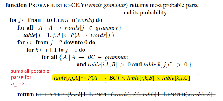
where notice that:

we don’t need to only store the max, we are summing over all possible ones for each parse $A_i$
we don’t need to store backtrack matrix because we are only spitting out a score

PCFG Learning

Lastly, we talk about how to learn those probabilities in the CFG rule in the first place. In general, there are two approaches:

when given some labelled training corpus (i.e. Treebank corpus, where parse trees are given), we just need to do counts. This is as simple as:
\[P(A \to \beta |A) = \frac{\text{Count}(A \to \beta)}{\text{Count}(A)}\]
again, since it is counts, we will need smoothing techniques.
if we don’t have a treebank but we do have a (non-probabilistic) parser, we can generate the counts and probabilities we need by
1. parsing a corpus of sentences with some nonprobabalistic parser to generate all possible parses (given the CNF productions)
  - of if only the set of non-terminals are provided, first generate all possible CFG rules and treat them as given
2. count for each parse of a sentence and weight each of these counts by the probability of the parse it appears in. But we dont’ have the probability to begin with! Hence the idea is then to use a EM like algorithm at this step.
  
  So we begin with a parser with equal rule probabilities.
3. Use EM to iteratively train the probabilities of these productions to locally maximize the likelihood of the data.
  1. parse the sentence, compute a probability for each parse
  2. use these probabilities to weight the counts, re-estimate the rule probabilities
  3. repeat until convergence

Note: If you don’t even have the set of non-terminals to start with, i.e. without the set of non-terminal fixed, the learning of CFG itself might be exponential as you need to try every possible non-terminals + every possible productions.

Problems with PCFG

While probabilistic context-free grammars are a natural extension to context-free grammars, they have two main problems as probability estimators:

Poor independence assumptions: CFG rules impose an independence assumption on probabilities (i.e. Markov) that leads to poor modeling of structural dependencies across the parse tree
- Recall that in a CFG the expansion of a non-terminal is independent of the context
Lack of lexical conditioning: CFG rules don’t model syntactic facts about specific words, leading to problems with subcategorization ambiguities, preposition attachment, and coordinate structure ambiguities.
- basically the problem in section Problems with CFG comes back here.

Because of these problems, probabilistic constituent parsing models use some augmented version of PCFGs, or modify the Treebank-based grammar in some way.

PCFG Independence Assumptions

Recall that in a CFG the expansion of a non-terminal is independent of the context, but in English the choice of how a node expands can after all depend on the location of the node in the parse tree.

For example, in English it turns out that NPs that are syntactic subjects are far more likely to be pronouns, and NPs that are syntactic objects are far more likely to be non-pronominal:

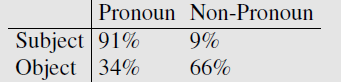
and there is no way to represent this in CFG as it is context free, so all we can do is:

\[\text{NP} \to \text{DT NN}, \quad 0.28 \\ \text{NP} \to \text{PN}, \quad 0.25\]

instead of something like “$\text{NP} \to \text{DT NN}= 0.91$ if it is in subject position”.

PCFG Lexical Dependencies Problem

A second class of problems with PCFGs is their lack of sensitivity to the words in the parse tree.

For example, consider the following problem of PP attachment: should it be to VP or NP? We have the following rules:

\[VP \to VBD\,\,NP\,\,PP\]

and

\[VP \to VBD \,\, NP\\ NP \to NP \,\, PP\]

It turns out that in some specific cases, the correct answer is with VP, but in other cases, the correct answer is with NP:

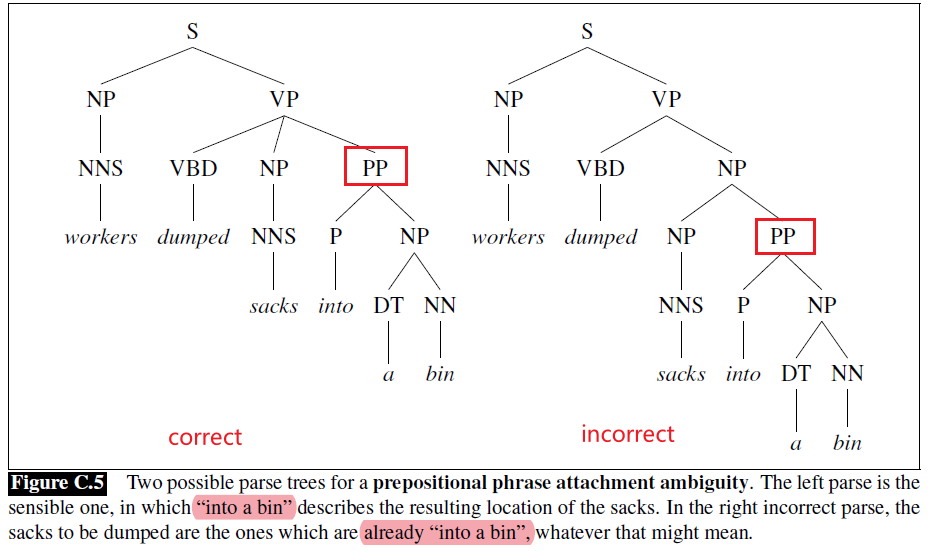
And with correct answer being with NP is when you analyze the sentence “fishermen caught tons of herring”, so that of is attached to tons, which is NP instead of attaching to caught.

Depending on how these probabilities are set, a PCFG will always either prefer NP attachment or VP attachment, hence missing one of the two correct parsing.

What information in the input sentence lets us know that when we need NP attachment while the other needs VP attachment? These preferences come from the identities of the verbs, nouns, and prepositions.

affinity between the verb dumped and the preposition into is greater, hence VP is preferred

affinity between the noun ton and ofis greater, hence NP is preferred

Thus, to get the correct parse for these kinds of examples, we need a model that somehow augments the PCFG probabilities to deal with these lexical dependency statistics for different verbs and prepositions in addition to what we have. (this will be done by using productions specialized to specific words by including their head-word in their LHS non-terminals)

PCFG with Splitting Non-terminals

Recall that the problem is CFG is context-free: what if NPs in subject position tend to be pronouns, whereas NPs in object position tend to have full lexical (non-pronominal) form.

One idea would be to split the NP non-terminal into two versions: one for subjects, one for objects: $NP_{\text{subject}}$ and $NP_{\text{object}}$. Then we can have:
\[NP_{\text{subject}} \to PR\\ NP_{\text{object}} \to PR\]
with two probability.

One way to implement this would be to do parent annotation

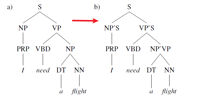
where, except for pre-terminal nodes, each non-terminal is labelled by X^Y where Y is the parent.

In addition to splitting these phrasal nodes, we can also improve a PCFG by splitting the pre-terminal part-of-speech nodes.

However, node-splitting is not without problems; it increases the size of the grammar and hence reduces the amount of training data available for each grammar rule, leading to overfitting. Thus, it is important to split to just the correct level of granularity for a particular training set.

PCFG with Lexicalization

Recall that another problem is to capture the fact that which production rule is better (disambiguation) also depends on the specific tokens/words/phrase, e.g. whether if PP should follow NP or VP.

Instead of using the above idea of splitting non-terminals = adding more syntax rules, here we add/allow for lexicalized rules.

The resulting family of lexicalized parsers includes the Collins parser (Collins, 1999) and the Charniak parser (Charniak, 1997).

Here the idea is that, since syntactic constituents could be associated with a lexical head, and we defined a lexicalized grammar in which each non-terminal in the grammar tree is annotated with its lexical head,

lexical head: one word which represents the crux of the underlying constituent

For instance, instead of $VP \to VBD \,\, NP\,\,PP$ we have:

\[VP(\text{dumped}) \to VBD(\text{dumped}) \,\, NP(\text{sacks})\,\,PP(\text{into})\]

for the following tree:

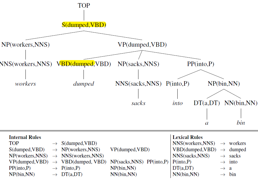
which also made a further extension to include the head word tag, e.g.

\[VP(\text{dumped}, VBD) \to VBD(\text{dumped}, VBD) \,\, NP(\text{sacks},NNS)\,\,PP(\text{into},P)\]

notice that the rules here have to be split into two sets:

lexical rules will be deterministic, since $p[DT(\text{a},DT) \to \text{a}] = 1$
internal rules with be probabilistic as usual. Those are the parameters we need to train.

Then, to train it, we can imagine this as a simple context-free grammar with many copies of each rule, one copy for each possible headword/head tag for each constituent. For instance, the rule:

\[VP(\text{dumped}, VBD) \to VBD(\text{dumped}, VBD) \,\, NP(\text{sacks},NNS)\,\,PP(\text{into},P)\]

should be estimated by:

\[\frac{\text{Count}[VP(\text{dumped}, VBD) \to VBD(\text{dumped}, VBD) \,\, NP(\text{sacks},NNS)\,\,PP(\text{into},P)]}{\text{Count}[VP(\text{dumped}, VBD) ]}\]

but obviously this is too specific. The idea of lexicalized parsing is to make some further independence assumptions to break down each rule so that we would estimate the probability, and an example would be the Collins Parser.

Although this can make disambiguation between parses work even better, accurately estimating parameters (i.e. probability of each of those production rules) on such a large number of very specialized productions could require enormous amounts of treebank data.

Simplified Collins Parser

In short, there we consider estimating the probability using some generative rules. This new generative story is that given the left-hand side:

We also add a special STOP non-terminal at the left and right edges of the rule;
we first generate the head of the rule
generate dependents on the left side of the head until we’ve generated on the left side of the head STOP
move to the right side of the head and start generating dependents there until we generate STOP.

Therefore, consider estimating:

\[P[VP(\text{dumped}, VBD) \to \text{STOP}\,\,\,\, VBD(\text{dumped}, VBD) \,\, NP(\text{sacks},NNS)\,\,PP(\text{into},P)\,\,\,\, \text{STOP}]\]

Then the generative procedure is:

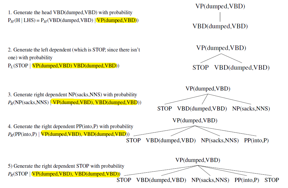
where notice that

except from the first node, all nodes are generated conditioning on $LHS,H$.
being left of the tree or right of the tree also matters!

Then, we can estimate the probability by a product:

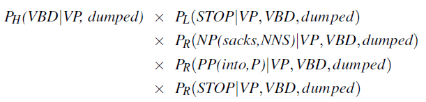
and each smaller probability can be estimated using counts, for example $P_R[NP(\text{sacks}) \vert VP,VBD, \text{dumped}]$ will be estimated by:

which is much less specific.

Evaluating Parsers

The standard tool for evaluating parsers that assign a single parse tree to a sentence is the PARSEVAL metrics

The PARSEVAL metric measures how much the constituents in the hypothesis parse tree (returned by your parser) look like the constituents in a hand-labeled, reference parse (given label).

Constituent in a hypothesis parse $C_h$ of a sentence $s$ is labeled correct if there is a constituent in the reference parse $C_r$ with the same starting point, ending point, and non-terminal symbol

For instance:

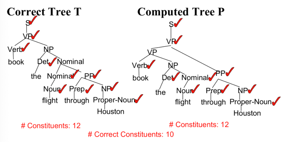
so in short a constituent basically corresponds to the word/leaves it entails + the label itself. Then, we can measure precision and recall

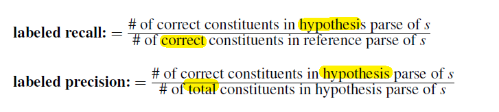
This is essentially related to the evaluation metric used in Chunking Algorithms. Therefore, the in this example will have:

\[\text{Recall} = 10/12\\ \text{Precision} = 10/12\]

And normally we report the $F_1$ score being:

\[F_1 = \frac{2P\cdot R}{P+R}\]

Results of current state-of-the-art systems on the English Penn WSJ treebank are $91\%-92\%$ labeled $F_1$.

We may also additionally use a new metric, crossing brackets, for each sentence $s$.

cross-brackets: the number of constituents for which the reference parse has a bracketing such as $((A B) C)$ but the hypothesis parse has a bracketing such as $(A (B C))$.

Human Parsing

Another idea for building a parser would be to think about how human parses a sentence.

Psycholinguistic studies show that words that are more probable given the preceding lexical and syntactic context are read faster. For instance:
\[\text{John put the dog inthe pen with a \textbf{lock}}.\]
where the last word should come pretty fast.

Then, modeling these effects requires an incremental statistical parser that incorporates one word at a time into a continuously growing parse tree.

Some additional problems that we need to consider due to “human effects” are:

garden path sentences: people are confused by sentences that seem to have a particular syntactic structure but then suddenly violate this structure: a grammatically correct sentence that starts in such a way that a reader’s most likely interpretation will be incorrect. For instance:
\[\text{The old man the boat.}\]
When we read old followed by man they assume that the phrase the old man is to be interpreted as determiner – adjective – noun. When readers encounter another the following the supposed noun man (rather than the expected verb, as in e.g. The old man washed the boat),[a] they are forced to re-analyze the sentence.

Incremental computational parsers can try to predict and explain the problems encountered parsing such sentences.
nested expressions: nested expressions are hard for humans to process beyond 1 or 2 levels of nesting, for instance:
\[\text{The rat the cat the dog the boy owned bit chased died.}\]
to solve this, one way is to use center embedding, which is computing the equivalent “tail embedded” (tail recursive) versions are easier to understand:
\[\text{The boy owned a dog that bit a cat that chased a rat that died.}\]

Other Grammars

Other constituent parsers that use an alternative to CFG grammar:

Mildly Context-Sensitive Grammars:
- parses that use Combinatory Categorial Grammar (CCG)
- parsers that use Tree Adjoining Grammar (TAG)
Unification Grammars: in order to handle word-agreements better, each constituent has a list of features such as number, person, gender, etc, and the constraint is that combining two constituents mean their features must unify as well
- Expressive grammars and parses (HPSG)

Midterm

Material up to and including the PCFG section.

Four big questions in midterm, on:

LM, Spell Correction
Neural Networks, concepts and some basic optimization methods
POS tagging (HMMs)
Syntactic Parsing, Statistical Parsing

Can bring cheat sheet. a double paged A4 paper.

Can bring a calculator.

Dependency Parsing

The focus of the two previous chapters has been on context-free grammars and constituent-based representations. Here we present another important family of grammar formalisms called dependency grammars.

Here, syntactic structure of a sentence is described solely in terms of directed binary grammatical relations between the words, as in the following dependency parse:

Relations among the words are illustrated above the sentence with directed, labeled arcs from heads to dependents.

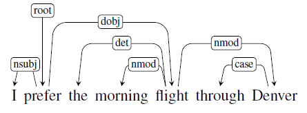
A major advantage of dependency grammars is their ability to deal with languages that are morphologically rich and have a relatively free word order. Though you can of course convert from a constituency parse tree to dependency tree, so they are related in some way.

For example:

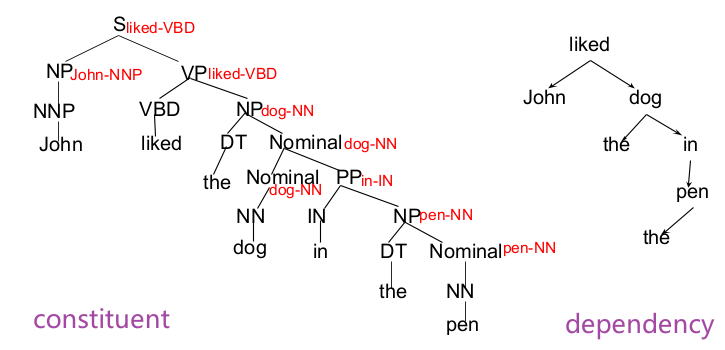
notice that:

the absence of nodes corresponding to phrasal constituents or lexical categories in the dependency parse; the internal/real structure of the dependency parse consists solely of directed relations between lexical items in the sentence.
so you can convert a phrase structure parse to a dependency tree by
- take each non-head child of a node
- make its parent to be the node with the head

Neural Shift-Reduce Parser

Deterministically builds a parse incrementally, bottom up, and left to right, without backtracking.

Shift Reduce Parsing

TODO

When each verb is encountered in the stack,

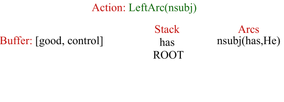
Neural Dependency Parser

Train a neural net to choose the best shift-reduce parser action to take at each step.

e.g. whether if you shoud left reduce or right reduce

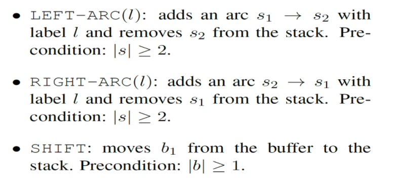
Use features (words, POS tags, arc labels) extracted from the current stack, buffer, and arcs as context.