Continuation from: NLP_part_1

Semantic Role Labeling

Here we consider solving the problem of, for each clause, determine the semantic role played by each noun phrase that is an argument to the verb.

We’ll introduce

semantic role labeling, the task of assigning roles to spans in sentences, and
selectional restrictions, the preferences that predicates express about their arguments, such as the fact that the theme of eat is generally something edible.

Examples would be:

Then, this would be useful as it can act as a shallow meaning representation that can let us make simple inferences that aren’t possible from the pure surface string of words:

Question Answering, e.g. “Who” questions usually use Agents
Machine Translation Generation

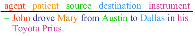
Semantic Roles

A variety of semantic role labels have been proposed, common ones are:

Agent: Actor of an action
Patient: Entity affected by the action
Instrument: Tool used in performing action.
Beneficiary: Entity for whom action is performed
Source: Origin of the affected entity
Destination: Destination of the affected entity

Although there is no universally agreed-upon set of roles, the above list some thematic roles that have been used in various computational papers

However, there are many problems with using those as-as. For instance, consider these possible realizations of the thematic arguments of the verb break:

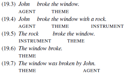
These examples suggest that break has (at least) the possible arguments AGENT, THEME, and INSTRUMENT.

The set of thematic role arguments taken by a verb is often called the thematic grid, q-grid, or case frame

An example would be for break:

Additionally, researchers attempting to define role sets often find they need to fragment a role like AGENT or THEME into many specific roles. And it has proved difficult to formally define the thematic roles. This essentially leads to two class of models for solution

define generalized semantic roles that abstract over the specific thematic roles.

For example, PROTO-AGENT and PROTO-PATIENT are generalized roles that express roughly agent-like and roughly patient-like meanings, and those roles are not defined by some “necessary tabular conditions”, but rather by a set of heuristic features that accompany more agent-like or more patient-like meanings.

Then the more an argument displays agent-like properties (e.g. being volitionally involved in the event), the more likely it is to be classified as PROTO-AGENT.
define semantic roles that are specific to a particular verb or a particular group of semantically related verbs or nouns

The first of them leads to the PropBank dataset, which uses both proto-roles and verb-specific semantic roles.

The second leads to FrameNet dataset, which uses semantic roles that are specific to a general semantic idea called a frame.

PropBank is a verb-oriented resource, while FrameNet is centered on the more abstract notion of frames, which generalizes descriptions across similar verbs.

Of course, both of which have sentences annotated with semantic roles.

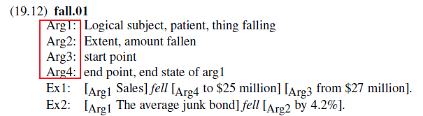
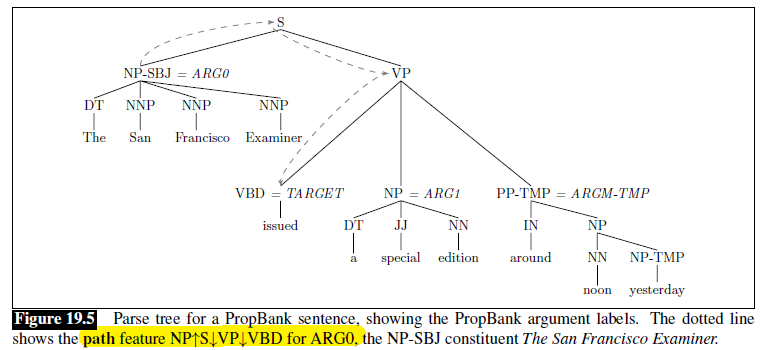
The Proposition Bank

Because of the difficulty of defining a universal set of thematic roles, the semantic roles in PropBank are defined with respect to an individual verb sense. Basically we have verb sense-specific labels (i.e. depending on the verb-sense, we will have different labels for arguments.)

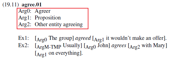
In general, we will use labels names: Arg0, Arg1, Arg2, and so on:

Arg0 represents the PROTO-AGENT
Arg1, the PROTO-PATIENT
Arg2 is often the benefactive, instrument, attribute, or end state
Arg3 the start point, benefactive, instrument, or attribute,
Arg4 the end point

Examples include:

| | | | ———————————————————– | ———————————— |

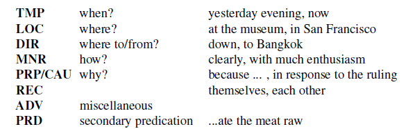
Additionally, PropBank also has a number of non-numbered arguments called ArgMs, (ArgMTMP, ArgM-LOC, etc.) which represent modification or adjunct meanings. As those are pretty much the same across verb senses, they are not listed with each frame file. However, they could be useful for training systems. Some examples of ArgM’s include:

FrameNet

Whereas roles in the PropBank project are specific to an individual verb, roles in the FrameNet project are specific to a frame.

A frame is basically the holistic background knowledge that unites these words, such as:

\[\text{reservation, flight, travel, buy, price, cost, fare}\]

all defined with respect to a coherent chunk of common-sense background information concerning air travel.

Therefore, FrameNet defines a set of frame-specific semantic roles, called frame elements, and includes a set of predicates that use these roles. (i.e. those roles of a word will be different across different frames)

additionally, FrameNet also codes relationships between frames, allowing frames to inherit from each other, or representing relations between frames like causation

For example, the change_position_on_a_scale frame is defined as follows:

This frame consists of words that indicate the change of an Item’s position on a scale (the Attribute) from a starting point (Initial value) to an end point (Final value).

And example sentences with their labels include:

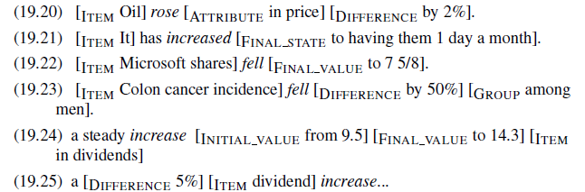
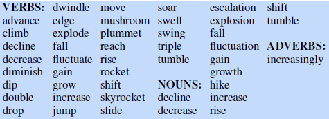
so if a word/verb (predicate) is in this frame, the above would be the labels. Verbs/predicates used in this frame looks like:

Semantic Role Labeling Models

Now we get to the task of Semantic role labeling (sometimes shortened as SRL): automatically finding the semantic roles of each argument of each predicate in a sentence. This is often done by:

supervised machine learning
using FrameNet and PropBank to specify predicates, define roles, and provide training and test sets.

Feature-based Algorithm for SRL

A simplified feature-based semantic role labeling algorithm basically do:

assign a parse (e.g. constituency parsing) of an input string
traverse the tree to find all predicates
for each node that is a predicate:
1. do a classification on that node, any standard classification algorithms can be used.
2. this can be done either by finding some feature representation of it, or using idea such as GNN

This results in a 1-of-$N$ classifier, i.e. where basically choosing one out of $N$ potential semantic roles (plus 1 for an extra None role for non-role constituents). The algorithm hence looks like:

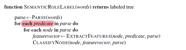
And the parse we did in step one could look like:

The general idea of those algorithms can be summarized into the following steps:

Pruning: Since only a small number of the constituents in a sentence are arguments of any given predicate, many systems use simple heuristics to prune unlikely constituents.
Identification: a binary classification of each node as an argument to be labeled or a NONE.
Classification: a 1-of-N classification of all the constituents that were labeled as arguments by the previous stage

However, since this labels each argument of a predicate independently, it is ingoing interactions between arguments, as we know the semantic roles are not independent.

Therefore, thus often add a fourth step to deal with global consistency across the labels in a sentence. This can be done by:

local classifiers can return a list of possible labels associated with probabilities for each constituent,
a second-pass Viterbi decoding or re-ranking approach can be used to choose the best consensus label.

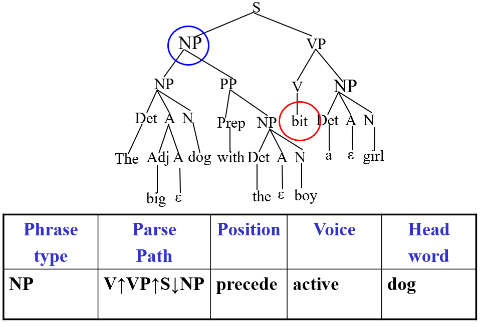
Features for Semantic Labelling Nodes

Common basic features templates mentioned above include

Phrase type: The syntactic label of the candidate role, the filler (e.g. NP).
Parse tree path: The path in the parse tree between the predicate and the candidate role filler.
Position: Does candidate role filler precede or follow the predicate in the sentence?
Voice: Is the predicate an active or passive verb?
Head Word: What is the head word of the candidate role filler?

An example would be for the predicate bit:

Problems that this method will suffer:

Due to errors in syntactic parsing, the parse tree is likely to be incorrect.
Can have many other useful features.

Neural Algorithm for SRL

A simple neural approach to SRL is to treat it as a sequence labeling task like named-entity recognition, using the BIO approach.

Assume that we are given the predicate and the task is just detecting and labeling spans. This means that we will have:

Input: sentence + the predicate, which will be separated by the SEP tag as shown in the example below
Output: semantic labels + BIO tags, as each label is a constituent (can span over more than one word)
- recall that BIO tags are: beginning, inside, outside.

An example architecture would be feeding it into a transformer:

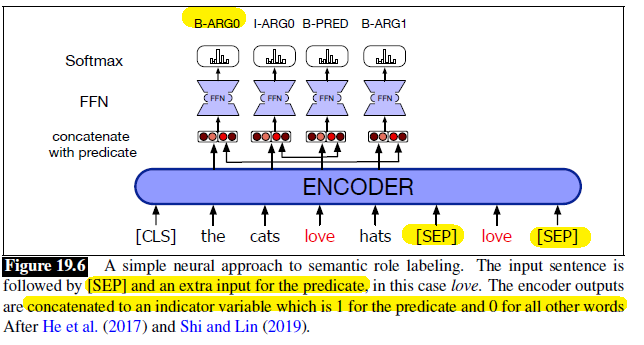
where of course those input word is mapped to pretrained embeddings.

Some problems that this method would encounter would be:

Results may violate constraints like “an action has at most one agent”?

Evaluation Metric for SRL

Since essentially we have Identification (should label or not) and Classification (which label), their performance can be evaluated separately:

each argument label must be assigned to the exact same parse constituent as in the ground truth
then, accuracy and recall can be used, for combined to look at F-score.

Selectional Restrictions

We turn in this section to another way to represent facts about the relationship between predicates and arguments.

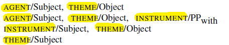
Frequently semantic role is indicated by a particular syntactic position . Examples include:

Agent: subject

Patient: direct object

Instrument: object of “with” PP

Beneficiary: object of “for” PP

Source: object of “from” PP

Destination: object of “to” PP

However, obviously this is not always correct.

\[\text{The hammer hit the window.}\]

then by the above logic hammer would be the AGENT, but it is actually an INSTRUMENT since it is not active.

Therefore, this means we also need to add Selectional Restrictions.

A selectional restriction is a semantic type constraint that a verb imposes on the kind of concepts that are allowed to fill its argument roles.

For instance, consider the following two sentences:

\[\text{I want to eat someplace nearby.}\\ \text{I want to eat Malaysian food.}\]

where both involve the predicate eat:

in the first case, we would want someplace nearby is an adjunct that gives the location of the eating event, instead of direct object
in the second case, we would want Malaysian food to be direct object, instead of adjunct

Therefore, we see that:

selectional restrictions are associated with senses, not entire lexemes
yet another way is to instead specify preference, i.e. which one is preferred instead of which one is deferred, which we will see soon.

This can be very useful in that it can rule out many ambiguities include:

Syntactic Ambiguity: “John ate the spaghetti with chopsticks.” would be wrong as PATIENTS of eat must be edible
Word Sense Disambiguation: “John fired the secretary.” vs “John fired the rifle.”

But of course, it is difficult to acquire all of the selectional restrictions and taxonomic knowledge and applying them is also a problem.

In reality, taxanomic abstraction hierarchies or ontologies (e.g. hypernym links in WordNet) can be used to determine if such constraints are met.

e.g. “John” is a “Human” which is a “Mammal” which is a “Vertebrate” which is an “Animate”

Selectional Preferences

Early word sense disambiguation systems used this idea to rule out senses that violated the selectional restrictions of their governing predicates. However, soon it became clear that these selectional restrictions were better represented as preferences rather than strict constraints.

Basically there will be measurements being a probabilistic measure of the strength of association between a predicate and a class dominating the argument to the predicate. More details see the book.

Advanced Semantics

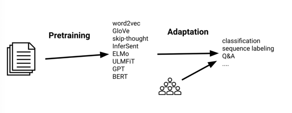
This section aims to give a quick recap of why we are using Pre-trained Language Models today for so many tasks.

A quick recap. We used pre-trained Embeddings to do:

e.g. skipgram word embeddings, compact dense representation for words
captures static semantic information of a word

Yet in reality, tasks we need to consider usually includes doing things after you got some embeddings. This means having NN such as RNN/transformer for downstream tasks such as sentiment analysis. However, there we also face problems if we want to train a model from scratch:

need a collection of data + manual labeling
often end up doing transfer learning: the training dataset is for move reviews, but for test we are working on Amazon product review

Simple Transfer Learning

The idea with word embedding to have a model learning some task agnostic data, and then fine tune it to task specific data.

This has been commonly used for fine-tuning word embeddings, but you will see that we can also have a model learn task agonistic objective (e.g. a language model), and then fine tune it for downstream task:

Then the advantage of pre-trained model in this setting would be:

no need of large corpus, only a few for fine-tuning
Can plug learned embeddings into the first layer

Additionally, for learning the task agnostic model, often:

No labelled data required – just a large text corpus and do self-learning such as masked word prediction or next word prediction

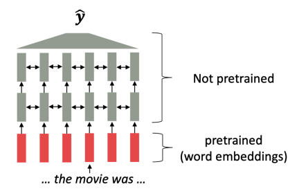
Problems with Pre-trained Word Embeddings

Why can we not just use the pretrained embeddings? (but use pretrained language models)

One assumption/property we had so far for a word embedding include:

they are static, hence does not care about the context, meaning the following would have the same
- “She broke the windshield with a bat.”
- “He was driving like a bat out of hell.”
word embedding before learnt from co-occurrence, which does not care about order!

However, for an entire network trained only tasks such as language model related ones:

Pretrained Word Embeddings	Pretrained Language Model

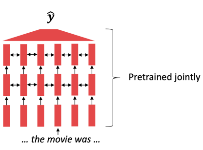then you basically remove the $\hat{y}$ layer and add a linear layer at the end for transfer learning.

e.g. include recurrent or Transformer layers to incorporate context
Better parameter initializations, for make it fine-tunable

Now, we discuss language model as a effective pretrain task (e.g. next word prediction, masked word prediction, etc)

It’s self-supervised, so there’s no need for labelled data. e.g. Large text collections are readily available on the web
it’s actually a difficult task, even for humans
- A model would need to learn about syntax, semantics, and even some world knowledge in order to do well at this task
- Luckily with a large number of parameters, large corpora, and lots of GPUs (or TPUs), we can do a pretty reasonable job

Neural Language Model

Recall: N-gram Language Model

The N-gram language model (e.g. for next word prediction) has limitations:

Sparsity (e.g. bigram matrix)
Need to store ngrams (and counts)
- Increases with n and corpus size
Don’t take into account word similarity

The solution to use Neural Language Model: predict the next word given the current context window

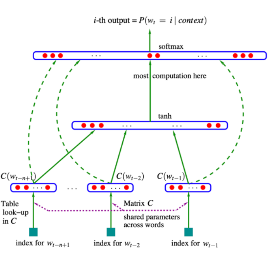
where the architecture is simply:

input -> embedding layer to start with
one or more intermediate layers, e.g. Linear, RNN, etc
output $\vec{h}$ and attach a SoftMax layer
- for fine-tuning the entire model, consider removing the softmax and attach another linear layer on top of $\vec{h}$ for your downstream task

This model solved several issues from N-gram models such as:

we have no sparsity problem
no need to store n-grams
can capture word-similarity via embeddings

However, several unsolved problems include:

Context window is limited (cannot just put in the entire document)
- Still can’t capture long range dependencies
Increasing context window == increasing parameters

LMs and Transfer Learning

Then the idea is that the LM task could be useful for any downstream task.

intuition: predict the next word positive fromthe sentence: the movie is great; positive”. Then we can use it as sentiment analysis

Therefore, you basically take the entire pre-trained model before the softmax layer as initialization, or as fine-tuning, or your downstream task. For instance:

use an pretrained LSTM LM on a large corpus
Use weights of embeddings and LSTM layers as initialization for the target task

Nowadays, besides LSTM LM, we have many pretrained architectures to choose from.

Architecture Choices

In NLP we have a lot of pretained language models. For each, be careful to consider the following aspects:

Model Architecture
Pre-training Objective
Pre-training Data
Adaptation to downstream tasks

Architecture Examples

In reality, since the pretained model has a lot of parameters, it is common to freeze those weights for the following models and add a linear/NN layer on top for your downstream task.

GPT

Transformer decoder with 12 layers
- 768 hidden units, 12 heads, 3072-dim feed forward layer (117M params)
Pre-training objective: next word prediction
Data:
- BooksCorpus
- 7K unpublished books covering a variety of genres (800M words)
- Allows model to condition on long-range dependencies
For GPT-2 and GPT-3
- Larger models + more data = stronger LMs

then, the paper tested this model and applied to a variety of different downstream tasks.

BERT

Pre-training objective: masked word prediction + next sentence prediction
- LMs are unidirectional, but language understanding is bidirectional.
- next sentence prediction: whether if the next sentence follows from the previous sentence
12 layer transformer encoder, 768 hidden units, 12 attention heads = 110M parameters
Data
- BooksCorpus (800M words)
- English Wikipedia (2,500M words)
  - Text passages only
Training time
- 4 days on 4x4 or 8x8 TPU v2 slices
- ~$7K to train BERT Large

Input architecture looks like

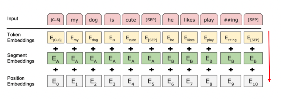
where:

segment embedding is to denote where we are putting the separator.

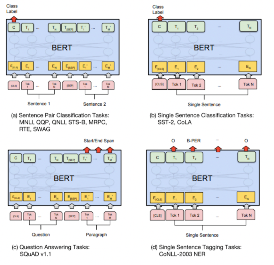
Then, using this model for other downstream tasks include

Some importnat variants of BERT:

RoBERTa
- Next sentence prediction not necessary as objective
- BERT + data + training steps
SpanBERT
- Mask out spans instead
  - e.g. which span of the reading/resource relates to the question that was asked
- Significant improvements on span selection tasks (such as QA)

It turns out that this also can be tuned for other languages: https://github.com/google-research/bert/blob/master/multilingual.md

Future of Pretrained Models

Currently the trend is

to have an increasing size of model and data:
consider zero/one/few-shot learning instead of transfer learning

Model size

BERT/GPT (2018) -> ~100M params
GPT-2 (2019) -> 1.5B params
T5 (2020) -> 11B param
GPT-3 (2020) -> 175B params

Dataset sizes

GPT (2018) -> 800M words
BERT (2018) -> 3B words
GPT-2 (2019) -> 40B words
GPT-3 (2020) -> 500B words

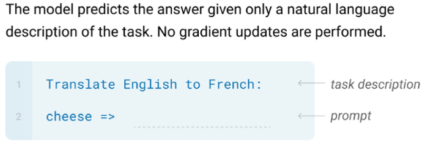
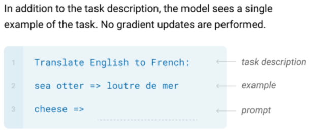
Additionally, different from the transfer learning paradigm, recently we have been looking at zero/one/few-shot learning

Zero-shot	One-shot	Few-hot

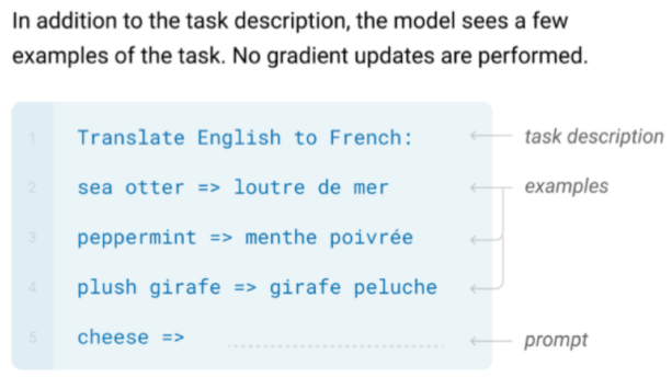one key difference here is that we do NOT update weights, we are only providing exmaples = providing a context.

Machine Translation

The task here is to translate one natural language into another. Some common usages include:

pure translation: Google translate

computer-aided translation: used to produce a draft translation that is fixed up in a post-editing phase by a human translator. This is commonly used as part of localization: the task of adapting content or a product to a particular language community

incremental translation: translating speech on-the-fly before the entire sentence is complete

Image-centric translation: use OCR of the text on a phone camera image as input to an MT system to translate menus or street signs

The standard algorithm for MT:

statistical methods (not used a lot today)
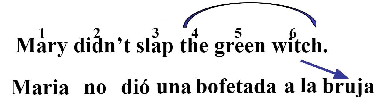
the encoder-decoder network, also called the decoder sequence to sequence network, an architecture that can be implemented with RNNs or with Transformers. Why can we not just use an encoder/just an decoder?

Machine Translation needs a map from a sequence of input words or tokens to a sequence of tags that are not merely direct mappings from individual words, which is exactly what such an architecture is doing.

An example of MT task would be:

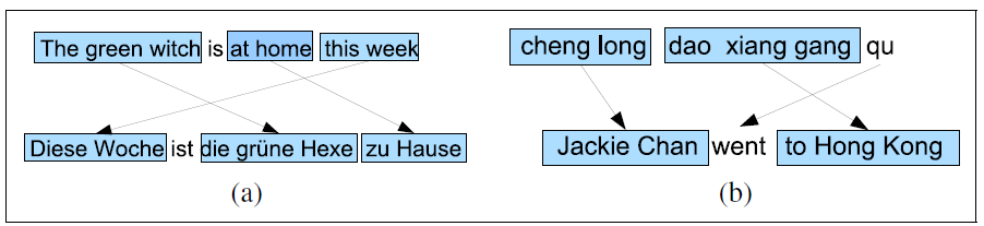
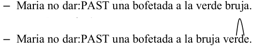
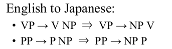
\[\text{English}: \quad \text{He wrote a letter to a friend}\\ \text{Japanese}: \quad \underbrace{\text{tomodachi}}_{\text{friend}}\,\,\underbrace{\text{ni tegami-o}}_{\text{to letter}}\,\,\underbrace{\text{kaita}}_{\text{wrote}}\]

which evinces some key challenges that makes the task difficult:

syntactical difference amongst languages: in English, verb is in the middle while in Japanese, verb is at the end.
- e.g. word ordering difference: SVO (e.g. English), SOV (e.g. Hindi), and VSO (e.g. Arabic) languages.
- e.g. In some SVO languages (like English and Mandarin) adjectives tend to appear before verbs, while in others languages like Spanish and Modern Hebrew, adjectives appear after the noun
Pro-drop languages: regularly omit subjects that must be inferred.
- e.g. Chinese sometimes drop subjects
Morphological difference
Lexical gaps: there might not exist a one to one mapping for a word in foreign languages

Encoder-decoder networks are very successful at handling these sorts of complicated cases of sequence mappings.

Indeed, the encoder-decoder algorithm is not just for MT; it’s the state of the art for many other tasks where complex mappings between two sequences are involved:

summarization (where we map from a long text to its summary, like a title or an abstract)
dialogue (where we map from what the user said to what our dialogue system should respond)
semantic parsing (where we map from a string of words to a semantic representation like logic or SQL)
and many others.

However, the current translation quality is not perfect:

Existing MT systems can generate rough translations that at least convey the gist of a document
High quality translations possible when specialized to narrow domains, e.g. weather forecasts.

Language Divergence

This section discusses a bit more on the differences between languages that makes the task of MT difficult

Languages differ in many ways, and an understanding of what causes translation such divergences will help us build better MT models. The study of these systematic cross-linguistic similarities and differences is called linguistic typology

Word Order Typology

As we hinted it in our example above comparing English and Japanese, languages differ in the basic word order:

Subject-Verb-Object order
In some SVO languages (like English and Mandarin) adjectives tend to appear before verbs, while in others languages like Spanish and Modern Hebrew, adjectives appear after the noun

Visual example of word order difference hence complex mapping:

Lexical Divergences

Here we need to deal with problems such as:

appropriate word/translation can vary depending on the context.
- e.g. German uses two distinct words for what in English would be called a wall: Wand for walls inside a building, and Mauer for walls outside a building.
Sometimes one language places more grammatical constraints on word choice than another.
lexical gap: no word or phrase, short of an explanatory footnote, can express the exact meaning of a word in the other language.

Morphological Typology

Recall that a morpheme is the smallest unit of meaning that a word can be divided into.

Then, in many languages we have:

difference in the number of morphemes per word
- isolating languages like Vietnamese and Cantonese, one morpheme per word
- polysynthetic languages like Siberian Yupik (“Eskimo”), in which a single word may have very many morphemes, corresponding to a whole sentence in English
difference in the degree a morpheme is separable
- agglutinative languages like Turkish, in which morphemes have relatively clean boundaries
- fusion languages like Russian, in which a single affix may conflate multiple morphemes

This means that translating between languages with rich morphology requires dealing with structure below the word level, .e.g. use subword models such as BPE.

Rule-Based MT Model

Rules-based machine translation (RBMT) is a machine translation approach based on hardcoded linguistic rules. The rules used here would include:

lexical transfer
lexical reordering
etc.

Direct Transfer

The task is to use rules to translate between, e.g. English to Spanish:

Use morphological analysis
Use lexical transfer rules to find syntactic one to many mapping of the translation of each word:

notice that here we did two things: do the translation per word (e.g. using a dictionary) + translated into basic grammar structure in Spanish
Lexical Reordering: fixing some more detailed word orders
Morphological generation: generate the morphology back from the first step

But of course even this rule-based approach has shortcomings in quality:

lexical reordering does not adequately handle more dramatic reordering such as that required to translate from an SVO to an SOV language. This means we need syntactic transfer rules that map parse tree for one language into one for another.

For example:
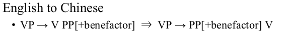
some transfer requires semantic information. For example, in Chinese PP expressing a goal semantically should occur before verb, but in English, it occurs after the verb.

Hence we need rules such as

Statistical MT

Of course rule-based approach have big problems

difficult to come up with good rules between two languages
it does not scale as it requires hand-written rules.

Instead of rule based direct transfer, consider a statistical model which at least scales

SMT acquires knowledge needed for translation from a parallel corpus or bitext that contains the same set of documents in two languages.

Noisy Channel Model

The idea is to consider, for example translating French to English:

Source sentence (e.g. French) was generated from some noisy transformation of the target sentence (e.g. English), as we have done in Spelling Correction.

Therefore, we consider finding the translation $\hat{E}$:

\[\hat{E} = \arg\max P(E |F)\]

for $F=f_1,f_2…,f_m$ being a sentence in French composing $m$ words, and $E = e_1,e_2,…,e_n$ being a sentence in English composed of $n$ words. Then using Bayesian rules:

\[\hat{E} = \arg\max_E P(E|F) = \arg\max_E \underbrace{P(F|E)}_{\text{likelihood of $E$}}\quad\underbrace{P(E)}_{\text{prior of $E$ occuring}}\]

where $P(F\vert E)$ would then be computed by a translation model and $P(E)$ by a language model.

e.g. $P(E)$ could come form a n-gram model. or a PCFG which captures syntactic structure as well, etc.
to compute $P(F\vert E)$, we would ideally want to do:
- find phrase alignments from a given $E$ to $F$ and translate each phrase
- but this is hard to do, so in reality we consider word alignment $A=a_1,…,a_k$ then translation
\[P(F|E) = \sum_A P(F|E,A)P(A|E)\]
more details on how this works is covered in the next section.

Word Alignment for MT

Recall that our task is to compute $P(F\vert E)$, for $F$ being a random variable and $E$ of length $n$.

To simplify the problem, typically assume the following:

where notice that:

given a $E$, each word in $E$ aligns to one or more words in $F$

each word in $F$ aligns to 1 word in $E$ (so it is a vector, as shown below)

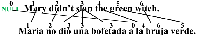
Then, an alignment in basically becomes a size $9$ vector which looks like:
\[[1,2,3,3,3,0,4,6,5]^T\]
which is for each word in $F$, the index of the word in $E$ which generated it. (then you can apply word-word level translation)

In general, such an alignment can be learnt from

supervised word alignments, but human-aligned bitexts are rare and expensive to construct.
so typically obtained using an unsupervised EM-based approach to compute a word alignment from unannotated parallel corpus.

IBM Model 1

Now, assume that $P(F\vert E,A)$ is computable. The IBM model for SMT can generated a single $F$ from $E=e_1,…,e_n$ of length $n$ by:

choose length $k$, so that we would have $F=f_1,…,f_k$
choose an alignment $A=a_1,…,a_k$ which represents which English word it should comes from
For each position of word in $F$, generated a word $f_j$ from the aligned English version $e_{a_j}$

Next, we can define how to compute $P(F\vert E)$ of $E$ having length $n$ by:

given some length distribution $P(K=k\vert E)$
assuming all alignments are qually likely, then there are $(n+1)^k$ possible alignments. Hence:
\[P(A=a_1,...,a_k|E=e_1,...,e_n) = \frac{P(K=k|E)}{(n+1)^k},\quad \forall a_i\]
i.e. same probability if given the same length. e.g. $P(A=0,1,2\vert E)=P(A=1,0,2\vert E)$
Given some translation probability per word from $e_y \to f_x$, let it be $t(f_x\vert e_y)$ we then have:
\[P(F|E,A) = \prod_{j=1}^kt(f_j|e_{a_j})\]
where the alignment would be given by previous step
Finally, we sum over all possible alignments:
\[P(F|E) = \sum_A P(F|E,A)P(A|E) = \sum_A \frac{P(k|E)}{(n+1)^k} \prod_{j=1}^kt(f_j|e_{a_j})\]
where the alignments $A$ would vary both in length $k$ and in the elements/indices within an alignment of same length.

Typically use an unsupervised EM-based approach to compute a word alignment from unannotated parallel corpus, e.g. you could have $A=0,1,2$, $A=1,0,2$, $A=1,0,0,2$, etc.

notice that this is only a forward algorithm, so if we need to decode, this would be not very computational efficient.

Lastly, the decoding produce for finding the best alignment can be done by:

\[\hat{A} = \arg\max_A \frac{P(k|E)}{(n+1)^k} \prod_{j=1}^kt(f_j|e_{a_j}) = \arg\max_A \prod_{j=1}^kt(f_j|e_{a_j})\]

then, how do we maximize a product of terms? Since each term is independent, we can maximize it by maximizing each term independently. Hence:

\[\hat{a}_j = \arg\max_{i} t(f_j,e_i),\quad \forall j\]

which tells you which English word $f_j$ should align to.

of course you can compute this once you know all the probabilities $P(k\vert E), t(f_y\vert e_x)$.

HMM-Based Word Alignment

Obviously, one problem with IBM Model 1 is that it assumes all alignments are equally likely and does not take into account locality, e.g. next to each other words are likely to be next to each other in another language as well.

To solve this issue, HMM models can be used which models the jump width as hidden state, i.e. :

translate current word

decide which next word to jump to for translation

repeat from step 1

First, an example would be

Iteration 1	Iteration 3	Iteration 4

notice that:

the jump could jump to the current word itself, as there could be one-to-many mapping
the jump could jump both forward and backward discontinuously. E.g.

Therefore, now we can define what this model really is

Hidden states are current English word $e_i$ being translated

State transition would be modelling the jumps for the next word, which is $a_{ij}=P(s_i \to s_j)$

Observations are the translated French word $f_j$

Emission probability is therefore $b_j(f_i)=P(f_i\vert e_j)$, which is basically probability of translation from $e_j \to f_i$

Then this means that:

Observation likelihood $P(F\vert E)$ can be computed by the forward algorithm with HMM
Decoding $\hat{E}=\arg\max_E P(E\vert F)$ can be computed by Viterbi algorithm with HMM

Training Word Alignment Models

Both the IBM model 1 and HMM model require the following parameters

$P(f_i\vert e_j)$ probability of individual word translation (shown in the example below)
$P(K=k\vert E)$, length of target translation sentence

which can be obtained/trained on a parallel corpus to set the required parameters, including the specific ones such as:

for HMM Model, we also need $P(e_i)$ and $P(e_i \to e_j)$ being transition probabilities

In general

if we have a labelled/supervised (hand-aligned) training data, parameters can be estimated directly using frequency counts; e.g. sentence alignment. Which sentence in a corpus corresponds to which sentence is another corpus.

most often we have an unsupervised piece of parallel corpus. Then we need to estimate the probabilities using EM type algorithm.

A sketch of the algorithm looks like

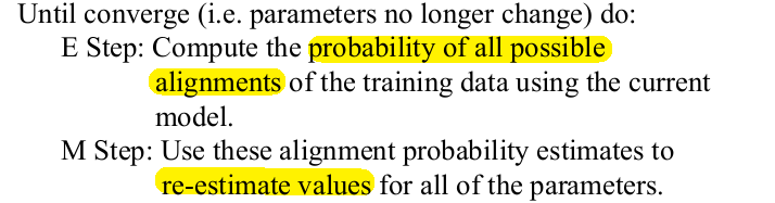
For example, given two data in the training corpus:

\[\text{green house} \iff \text{casa verde}\\ \text{the house} \iff \text{la casa}\]

Our aim is to be able to compute $P(s_i\vert e_j)$ for $s_i$ being a Spanish word, and perhaps vice versa.

notice that you should expect $\text{house} \iff \text{casa}$ to have a higher probability as this pair occurs more often

this is exactly what the EM algorithm tries to do

Step one: initialization. Here we can assume a uniform distribution such that each row/column sums to one

notice that each cell would represent $P(s_i\vert e_j)$ and vice versa.
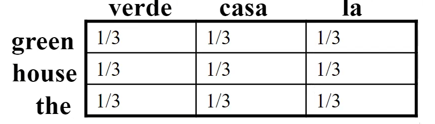
Expectation Step: we impute the missing data, which is to consider all possible alignments/individual translations. Here we have four possible cases:
\[\text{green} \iff \text{casa}\quad \text{AND} \quad \text{house} \iff \text{verde};\quad p=\frac{1/9}{2/9}=\frac{1}{2}\\ \text{green} \iff \text{verde}\quad \text{AND} \quad \text{house} \iff \text{casa};\quad p=\frac{1/9}{2/9}=\frac{1}{2}\]
and that
\[\text{the} \iff \text{la}\quad \text{AND} \quad \text{house} \iff \text{casa};\quad p=\frac{1/9}{2/9}=\frac{1}{2}\\ \text{the} \iff \text{casa}\quad \text{AND} \quad \text{house} \iff \text{la};\quad p=\frac{1/9}{2/9}=\frac{1}{2}\]
Maximization Step: then we fill in the table using the previous probabilities

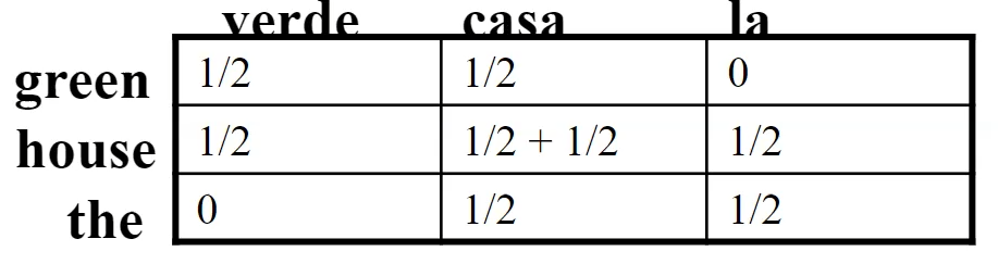
And normalizing to sum to one:
Repeat step 2-3 until convergence. Here just to be clear we show one more iteration of step 2. Possible alignments and their probability:

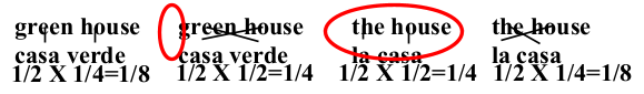
Hence
\[\text{green} \iff \text{casa}\quad \text{AND} \quad \text{house} \iff \text{verde};\quad p=\frac{1/8}{3/8}=\frac{1}{3}\\ \text{green} \iff \text{verde}\quad \text{AND} \quad \text{house} \iff \text{casa};\quad p=\frac{1/4}{3/8}=\frac{2}{3}\]
and
\[\text{the} \iff \text{la}\quad \text{AND} \quad \text{house} \iff \text{casa};\quad p=\frac{1/4}{3/8}=\frac{2}{3}\\ \text{the} \iff \text{casa}\quad \text{AND} \quad \text{house} \iff \text{la};\quad p=\frac{1/8}{3/8}=\frac{1}{3}\]

Note that the above works by the assumption that many words will be repeated.

Neural Machine Translation

As mentioned before, translation often involves a complex map between two sequences, hence usually we do

encoder-decoder model (e.g. LSTM blocks)

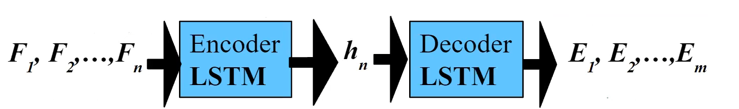
e.g. transformer based encoder-decoder
integrate an LSTM with language model using “deep fusion.”

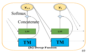
which basically is for decoder to predict the next word from a concatenation of the hidden states of both the translation and language LSTM models.

Evaluating MT

Translations are evaluated along two dimensions:

adequacy: how well the translation captures the exact meaning of the source sentence. Sometimes called faithfulness or fidelity.
fluency: how fluent the translation is in the target language (is it grammatical, clear, readable, natural).

The most accurate metric is to have human to score the translations based on the above criterion, but that is inefficient and expensive. This in reality is done often in the following manner:

Collect one or more human reference translations of the source, i.e. gold standard
Compare MT output to these reference translations.
Score result based on similarity to the reference translations.

Some automatic scoring system implemented today include BLEU, NIST, TER, etc.

BLEU

BLEU (Bilingual Evaluation Understudy): scores based on the following criteria:

What percentage of machine n-grams can be found in the reference translation?

Brevity Penalty: if translated sentence is too short, e.g. the., it matches/precision $1.0$ but it is cheating!

To answer the first question, an example would be:

finding shared unigrams:

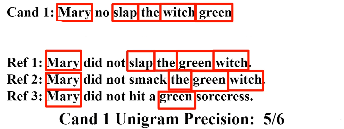
where basically we count a match if the unigram appears in at least one of the reference translation
finding shared bigrams
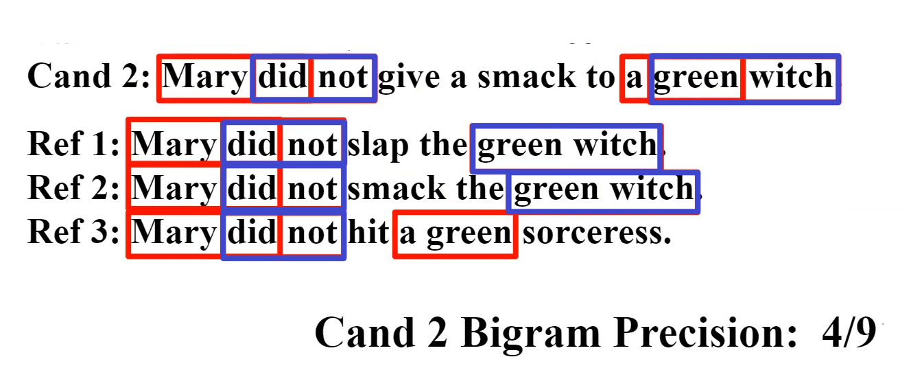
until some fixed size $N$, typically $4$.

Finally, scoring the first criteria involves finding a geometric mean:

\[\text{Precision}_{gm} = \sqrt[N]{\prod_{n=1}^NPr_n}\]

However, this alone will not work, because you can have a shorter sentence which would give a higher score. Therefore, we also need a brevity penalty/the second criteria:

ideally, we might compute $\text{Recall}$. which could solve the problem. But this is problematic since there are multiple alternative gold-standard references.
therefore, we cook up with the following metric:

Define effective reference length, $r$, as the length of the reference sentence with the largest number of n-gram matches. Then, if $c$ is the candidate sentence length:
\[BP = \begin{cases} 1,& \text{if }c > r\\ e^{1-(r/c)},& \text{if }c \le r \end{cases}\]

So that the final score is:

\[BLUE = \text{Precision}_{gm} \times BP\]

Challenges and Futures in MT

Certain challenges in MT include:

OOV word in test set. We need smoothing or other techniques, such as subword.
domain mismatch: e.g. corpus in movie but test in Amazon product review
translating long context is hard, even with attention it is not completely solved
low-resource language pairs
NMT can pick up biases (e.g. gender bias)

Some future directions include:

unsupervised MT attempts to learn language laignment form monolinguial data
multilingual NMT, learn shared representation across all languages (which can solve low resource problem)
Neural LSTM methods are currently the state-of-the-art.

Sentiment Analysis and Classification

In this chapter we introduce the algorithms such as Naïve text Bayes algorithm and apply it to text categorization, the task of assigning a label or category to an entire text or document. In particular, we focus on categorizing text based on its sentiments, i.e. sentiment analysis.

e.g. positive or negative orientation that a writer expresses toward some object.

simplest version of sentiment analysis is a binary classification task

Other commonly used names for sentiment analysis include: Opinion extraction; Opinion mining; Sentiment mining; Subjectivity analysis.

So now are are dealing with classification task, which is to be set in contrast to Seq2Seq task. Here we only need to output a single label/or a small fixed set for the entire document, e.g. a single written product review.

Other text categorization other than sentiment include:

Spam detection: another important commercial application, the binary classification task of assigning an email to one of the two classes spam or not-spam
Authorship attribution: whether if a given text is written by the person
Subject category classification: which library category does a piece of text belong to? Science? Humanities? etc.

The goal of classification is to take a single observation, i.e. a test sample, extract some useful features, and thereby classify the observation into one of a set of discrete classes.

And again recall that there are two broad class of classification algorithms:

Generative classifiers like Naïve Bayes
Discriminative classifiers like logistic regression

Real Life Example: Twitter posts sentiment analysis

For posts from Twitter:

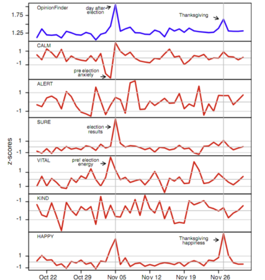
where we see “Happiness” surges around Election day and Thanksgiving. Other commonly used cases include:

Movie: is this review positive or negative?
Products: what do people think about the new iPhone?
Politics: what do people think about this candidate or issue?
Used as an input/feature to other task, such as predicting market trends from sentiment
etc.

Scherer Typology of Affective States

Some labels you can have for affective states human have:

Emotion: brief organically synchronized … evaluation of a major event
- angry, sad, joyful, fearful, ashamed, proud, elated
Mood: diffuse non-caused low-intensity long-duration change in subjective feeling
- cheerful, gloomy, irritable, listless, depressed, buoyant
- more for longer term predictions
Interpersonal stances: affective stance toward another person in a specific interaction
- friendly, flirtatious, distant, cold, warm, supportive, contemptuous
- used often for Social Media analysis, how users interact online between each other
Attitudes: enduring, affectively colored beliefs, dispositions towards objects or persons
- liking, loving, hating, valuing, desiring
- used a lot for product reviews and sentiment analysis
Personality Traits
- nervous, anxious, reckless, morose, hostile, jealous
- not very commonly used, but related to those personality test you take

Of course, which ones to use depends on the particular application.

Sentiment Analysis and Attitudes

Often sentiment analysis is framed as the detection of attitudes. In particular, we want to find out

Holder (source) of attitude
Target (aspect) of attitude
Type of attitude
- From a set of types: Like, love, hate, value, desire, etc.
- Or (more commonly) simple weighted polarity: positive, negative, neutral, together with strength
Text containing this attitude: which sentence/document

In reality:

Simplest task: Is the attitude of this text positive or negative? This will be our focus in this chapter as a classification task.
More complex: Rank the attitude of this text from 1 to 5, i.e. include strength
Advanced: all the 4 subtasks.

Sentiment Classification

Here we take on the simplest task: Is an IMDB movie review positive or negative?

For instance, we could have

Positive	Negative
When Han solo goes light speed , the stars change to bright lines, going towards the viewer in lines that converge at an invisible point . Cool.	“snake eyes” is the most aggravating kind of movie : the kind that shows so much potential then becomes unbelievably disappointing

In general, the steps we need to go through before and at classification time include:

Tokenization:
- Deal with HTML and XML markup
- Deal with Emoticons
- Deal with Twitter mark-up (names, hash tags), e.g. @xxx
Feature Extraction
- Some how handle negation, which could flip the meaning of a sentence:
  \[\text{I didn’t like this movie.}\quad v.s.\quad \text{I did like this movie.}\]
  one idea is to convert the former to:
  \[\text{I didn’t NOT\_like NOT\_this NOT\_movie}.\]
  basically adding NOT to every word between negative and the following punctuation.
- Then perhaps we don’t need all words? Only need the adjectives? (It turns out using All words work better)
Classification using different classifiers:
\[\text{class} = \arg\max_{c_j \in C} P(C|W=w_1,...,w_n)\]
- Naive Bayes
- MaxEntropy
- SVM

We will first introduce some baseline algorithms that works at least.

Baseline: Multinomial Naïve Bayes

Multinomial Naïve Bayes is essentially a Naive Bayes classifier that is able to output a class among many classes (more than two). This is essentially done by:

(assumption: Naive Bayes) probabilities $P(w_i\vert c)$ are independent given the class $c$. Therefore it allows

\[P(w_1,...,w_n|c_j) = \prod_i P(w_i|c_j)\]
hence
\[c = \arg\max_{c_j \in C} P(c_j) P(w_1,...,w_n |c_j) =\arg\max_{c_j \in C} P(c_j)\prod_i P(w_i |c_j)\]

So for Naive Bayes, we consider:

\[c = \arg\max_{c_j \in C} P(W|c_j)P(c_j) =\arg\max_{c_j \in C} P(c_j)\prod_i P(w_i |c_j)\]

meaning that we assume each word to be independently contributing to $c_j$. Note that

this is a generative model because this equation can be understood as:
1. generate a class $P(c_j)$
2. generate the words from the class $P(w_i\vert c_j)$
in many cases Naive Bayes is a linear classifier

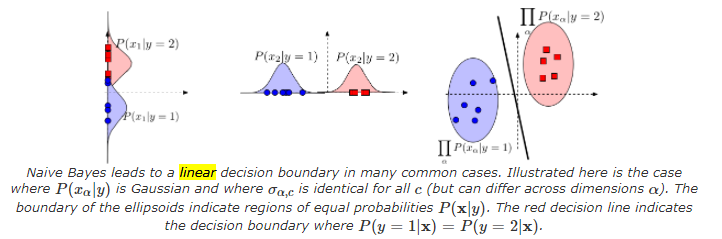
where you see the decision boundary for $P(c_1\vert x)=P(c_2\vert x)$ is a line.

To avoid numeric underflow, we would convert the estimate to log space:

\[c_{NB} = \arg\max_{c_j \in C} \,\,\log P(c_j) + \sum_i \log P(w_i|c_j)\]

But how do we learn $P(c_j)$ and $P(w_i\vert c_j)$?

learning the prior $P(c_j)$ is easy. Given $N_{doc}$ documents (e.g. posts), let $N_{c_j}$ be the number of document with sentiment class $c_j$. Then:
\[\hat{P}(c_j) = \frac{N_{c_j}}{N_{doc}}\]
learning the likelihood means counting how often is $w_i$ associated with class $c_j$. Hence we consider:
\[\hat{P}(w_i|c_j) = \frac{\text{Count}(w_i, c_j)}{\sum_{w\in V}\text{Count}(w_i, c_j)}\]
where:
- $\text{Count}(w_i, c_j)$ represent the number of times the word $w_i$ appears among all words in all documents of class $c_j$.
- In other words, we first concatenate all documents with class $c_j$ together, then count the number of occurrence of $w_i$.
- since eventually we need this for all words, $V$ presents the entire vocabulary instead of vocabulary in class $c_j$.

Since we are using count, consider smoothing as well for unmet $w_i,c_j$ pair:

\[\hat{P}(w_i|c_j) = \frac{\text{Count}(w_i, c_j)+1}{\sum_{w\in V}\text{Count}(w_i, c_j)+1}=\frac{\text{Count}(w_i, c_j)+1}{\text{Count(total words in $c_j$)}+|V|}\]

which is critically needed as the likelihood term is a multiplication.

for OOV words, we can use the technique introduced before by inducing OOV vocab in the training set. However, for Naive Bayes, it is more common to ignore those words completely (as if you didn’t see it)
other processing step include removing stop words such as a and the for both train and test sets. Though the performance gain from this is not significant.

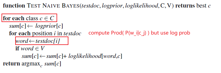
Therefore, the algorithm for learning is

Then for testing, we simply perform:

\[\hat{c} = \arg\max_{c_j \in C} P(c_j)\prod_i P(w_i |c_j)\]

Hence the algorithm for test is

Example

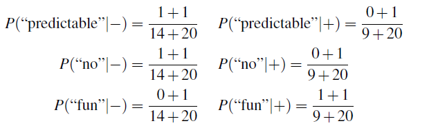
We’ll use a sentiment analysis domain with the two classes positive (+) and negative (-). The train and test set is provided below

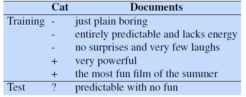
What are the parameters $P(c_j)$ and $P(w_i\vert c_j)$ in this case?

the prior $P(c_j)$ is simply counts:
\[P(-) = \frac{3}{5},\quad P(+) = \frac{2}{5}\]
then the smoothed likelihood essentially is
\[\hat{P}(w_i|c_j) = \frac{\text{Count}(w_i, c_j)+1}{\sum_{w\in V}\text{Count}(w_i, c_j)+1}=\frac{\text{Count}(w_i, c_j)+1}{\text{Count(total words in $c_j$)}+|V|}\]
where $\vert V\vert =20$ and we see that $\text{Count(total words in$+$)}=14$ and $\text{Count(total words in$-$)}=9$. Hence some examples:

and the rest is trivial.

For estimation, first we realize that the word with is OOV. Hence we ignored it as we are doing Naive Bayes. Then we are basically predicting $\text{“Prediction no fun”}$:

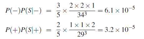
hence the result is $-$ as it has a higher probability.

Improvements From Baseline

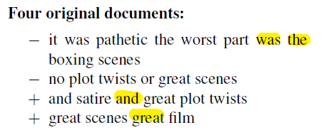
While standard naive Bayes text classification can work well for sentiment analysis, some small changes are generally employed that improve performance.

does the $\text{Count}(w_i,c_j)$ really matters? Maybe all it matters is that fact that it occurred in $c_j$ document at least once!
dealing with negation improves Naive Bayes accuracy as well:
\[\text{I didn’t like this movie.}\quad v.s.\quad \text{I did like this movie.}\]
notice that the negation of didn’t completely changed $P(\text{like}\vert c_j)$, for instance. The baseline that deals with this is mentioned before by converting them to
\[\text{I didn’t NOT\_like NOT\_this NOT\_movie}.\]
where newly formed words such as $\text{NOT_like}$ will be treated as a word.
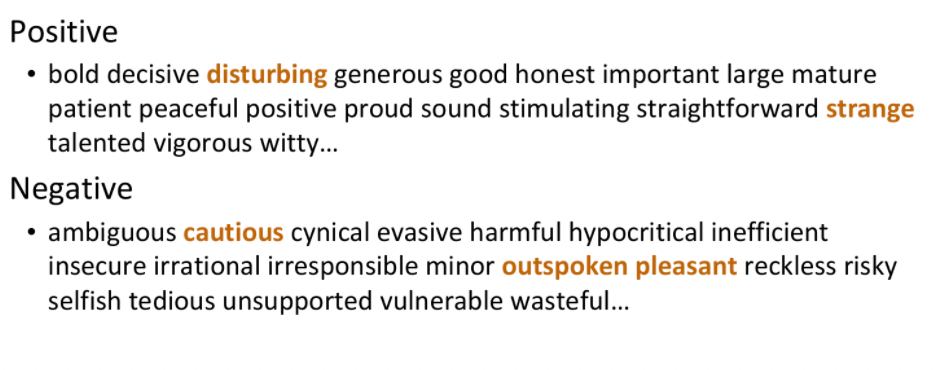
insufficient labeled training data to train accurate naive Bayes classifiers using all words in the training set. In those cases we will have to derive word features (e.g. labelled emotion carried in a word) using sentiment lexicons. Some popular ones online include:
- General Inquirer, LIWC, The Opinion Lexicon, MPQA
- example of annotated words from MPQA include:
  \[+ : admirable, \,\,beautiful, \,\,confident, \,\,dazzling, \,\,ecstatic,\,\, favor,\,\, glee,\,\, great\\ - : awful,\,\, bad,\,\, bias,\,\, catastrophe, \,\,cheat, \,\,deny,\,\, envious,\,\, foul,\,\, harsh, \,\,hate\]
  A common way to use lexicons in a naive Bayes classifier is to add a feature that is counted whenever a word from that lexicon occurs.

Here we will go over details on how to implement the Binary NB variant.

If we believe that word occurrence may matter more than word frequency: then we can do “Binary Naive Bayes”, which clips all the word counts in each document at $1$. (i.e. it’s like a Boolean switch for each word)

this results in binary multimodal naive Bayes, or binary NB

in practice this seems to be true, that performance is better.

In algorithm, basically you can first reduce all duplicate words in each document to one occurrence, and then perform the same algorithm.

For example:

Raw Naive Bayes	Boolean Naive Bayes

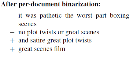where the highlighted words are duplicates within the document. Hence the counts become:

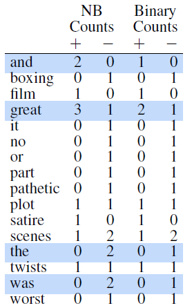
Then for testing, the we do not remove words as this is just for making the probability work better.

Problems in Sentiment Classification

Some cases where Naive Bayes’ assumption essentially fails:

Subtlety in words: each word itself is neutral, but overall there is a sentiment:

“If you are reading this because it is your darling fragrance, please wear it at home exclusively, and tape the windows shut.”
Thwarted Expectations and Ordering Effects: where words such as However would suddenly change the sentiment

“This film should be brilliant. It sounds like a great plot, the actors are first grade, and the supporting cast is good as well, and Stallone is attempting to deliver a good performance. However, it can’t hold up.”

In those cases just modelling $P(w_i\vert c_j)$ won’t work. Neural Models that remember/see contexts would work better.

Polarity in Sentiment Analysis

Here, the idea is that each word/phrase themselves could have polarity, meaning that they themselves could be indicative of the sentiment of the sentence/document.

Polarity is float which lies in the range of $[-1,1]$ where $1$ means positive statement and $-1$ means a negative statement.

Some simple measurement of such is to consider:

how likely each word is to appear in each sentiment class (discussed here)
use some form of embedding, which could be learnt in a Word2Vec approach

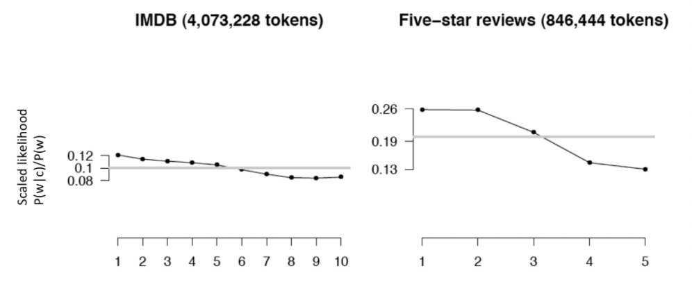
For instance, consider the polarity of the word “bad”:

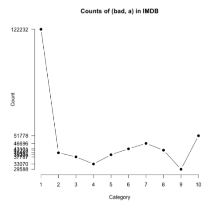
where

each category $c$ would represent the word “bad” appearing in a 1-star, 2-star, 3-star review, etc
notice that even in 10-star comments, we still see the word “bad” quite often. This could happen due to negations.

Then, since we have the counts, we can compute the likelihood

\[P(w|c) = \frac{\text{Count}(w,c)}{\sum_{w}\text{Count}(w,c)}\]

where $c$ would represent 1-star, 2-star, … Then we could scale it so it is comparable between words

\[\frac{P(w|c)}{P(w)}\]

for $P(w)$ would be a the probability of observing the word at all.

Exmaple: Polarity of each word in IMDB

Plotting the scaled likelihood for some common words in the 1-10 star IMDB reviews look like:

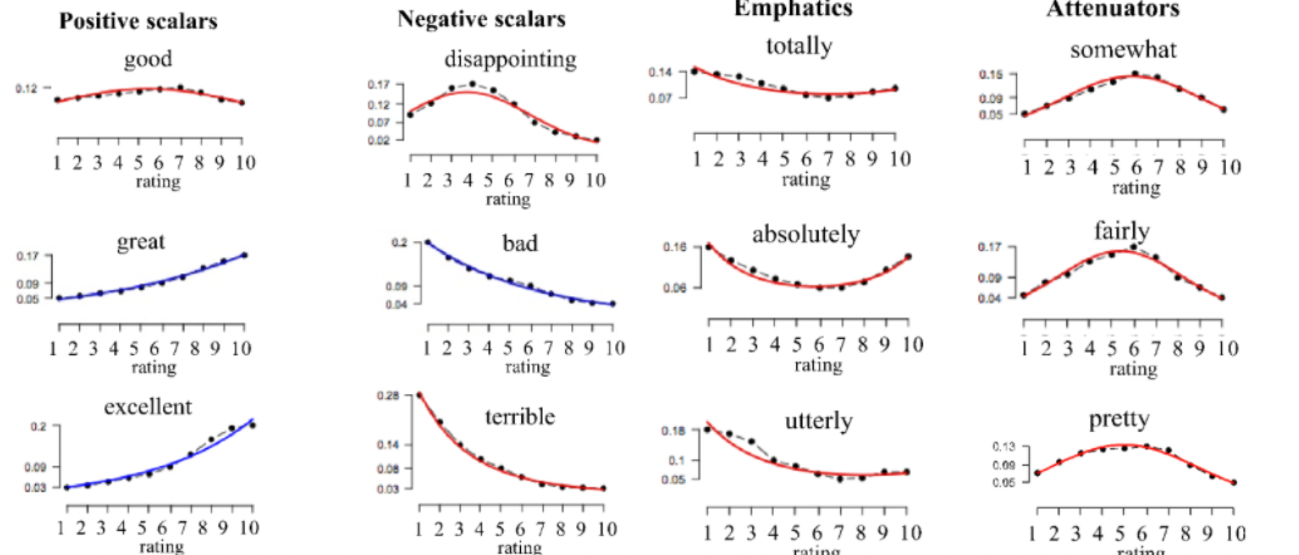
where:

notice that “good” looks relatively flat across ratings (perhaps due to negations). This means “good” is not a good indicator for positive sentiment/rather neutral polarity.
words such as “great” and “excellent” would be a better “metric” for the positive rating of the movie/positive polarity.
words such as “somewhat” and “fairly” are attenuators as they most happen in th middle of the rating; they dampen extremely positive/negative reviews
the upshot is that even seemingly positive/negative words could happen in all contexts

Logical Negation and Polarity

Is logical negation (no, not) associated with negative sentiment? (we know there are problematic cases such as “I don’t hate this movie” is a positive review with double negative.)

In general, there are slightly more negation in negative sentiments. For word such as “no/not”, the plot looks like:

where notice that:

the scaled likelihood is slightly higher for low ratings for negation word such as “no/not”
so even if we have double negatives such as “I don’t hate this movie”, this is still a useful feature

Learning Sentiment Lexicons

Here we consider the case that you want to have some sort of word polarity for your domain task, but there is no dataset with lexicons and ratings so that you cannot really know which words are more positive/negative.

e.g. maybe dealing with a academic domain, where polarity of words would be different from well-established datasets such as movie reviews

Can we use a few hand-built patterns/lexicons to bootstrap and build a larger lexicon list?

more lexicons learnt means your model could be more robust to test set

useful for domain transfer

The general idea/a simple rule:

adjectives conjointed by “and” tend to have same/similar polarity. e.g. “fair and legitimate”
adjectives conjointed by “but” tend to have different polarity. e.g. fair but brutal

Then, we can consider some kind of program that does:

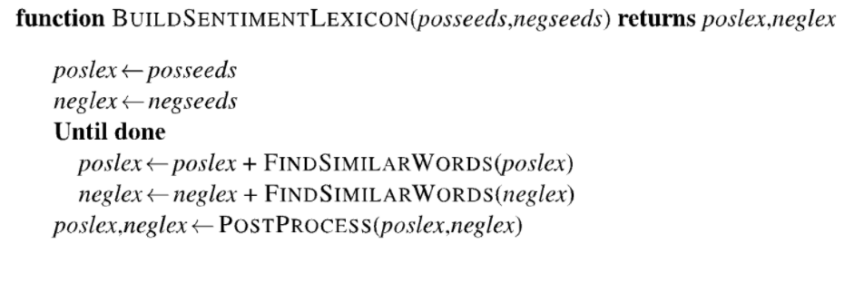
where seeds are the hand-built small lexicon list you made. Now, the question become:

Where do you find similar/different words? Use a database or search engine!

Example:

Start with a labelled seed set of words. For instance a labelled seed set of 1336 adjectives such that:
- there are 675 positive ones: adequate, central, clever, etc.
- there are 679 negative ones: contagious, drunken, ignorant, etc
Then we can find similar words from a database/a search engine by conjoining with “and”:
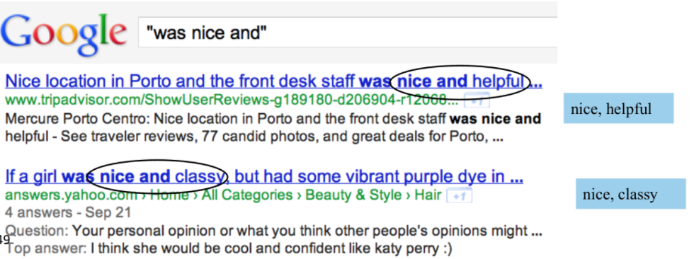
However, words might appear in many pairs. For instance, we could have a “fair and nice”, and but possibly “fair and corrupt” as well.

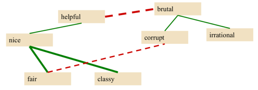
Therefore, from the seed set, we can train a supervised classifier to assign a polarity similarity score to a given pair of word.
Then we can determine the cluster by:
- for any two pair, if unknown polarity similarity, use the trained classifier
- closer polarity words are grouped/clustered together
Hence we would arrive at:
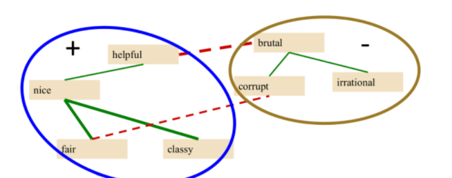
Output the clusters and words inside it

note that of course we can get errors.

Turney Algorithm

Notice the above is a semi-supervised approach to learn a lexicon list with polarity. Then with those polarity, we could potentially use to classify sentiment of documents containing those words.

However, is there are way to do it in a unsupervised approach?

Unsupervised classificaiton of reviews! Done by:

Extract a phrasal lexicon from reviews (following some pre-defined rules)

Learn polarity of each phrase (by co-occurance with words such as “excellent” and “poor” )

Rate a review by the average polarity of its phrases

For computation and simplicity, we only extract two-word phrases with adjectives. Then, the algorithm does

First we extract the phrases. We extract two-word phrases that satisfy the following POS tags:

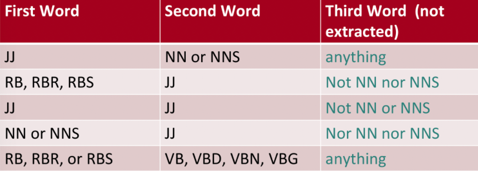
note that RB, RBR, RBS are the comparitive/superlative form of adjectives JJ.
Then we need to know the polarity of phrase. We hypothesize that:
- Positive phrases co-occur more with “excellent”
- Negative phrases co-occur more with “poor”
- the choice of the two words should at least come from the graphs in section Polarity in Sentiment Analysis
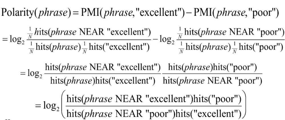
We can measure the co-occurance by PMI, which comes from a co-occurance matrix. Recall that it is a measure of how often two events $x$ and $y$ occur together, compared with what we would expect if they were independent:
\[I(x,y) = \log_2\left(\frac{P(x,y)}{P(x)P(y)}\right)\]
Hence, the pointwise mutual information between a target word $w$ and a context word $c$ (for some window size such as 7) is then defined as:
\[\text{PMI}(w,c) = \log_2\left(\frac{P(w,c)}{P(w)P(c)}\right)\]
for probabilities can be estimated with word-context matrix, we consider target words $w$ and context $c$. In this case, we don’t really care about context but rather how often $w$ appears with “excellent” and “poor” as:
\[\text{PMI}(w, \text{excellent}) = \log_2\left(\frac{P(w,\text{excellent})}{P(w)P(\text{excellent})}\right)\]
and similarly for “poor”. Then:
- To get those counts and the co-occurance matrix, we will use the search engine:
  \[\hat{P}(w) = \frac{\text{hits}(w)}{N}, \quad N=\sum_w \text{hits}(w)\]
  Then $\hat{P}(w_1, w_2)$ can be esitmated by:
  \[\hat{P}(w_1, w_2) = \frac{\text{hits}(w_1\,\, \text{Near}\,\, w_2)}{\sum_{w_1, w_2}\text{hits}(w_1\,\, \text{Near}\,\, w_2)}=\frac{\text{hits}(w_1\,\, \text{Near}\,\, w_2)}{kN}\]
  for $k$ being the size of the window, i.e. being $k$ words apart. (we often drop $k$ in subsequent calculation as it is a constant)
- Finally, the PMI is therefore
  \[\text{PMI}(w, \text{excellent}) = \log_2\left(\frac{\text{hits}(w_1\,\, \text{Near}\,\, w_2)/N}{\text{hits}(w)\text{hits}(w_2)/N^2}\right)\]
Finally, we define the polarity of a phrase by doing the PMI difference between "*excellent*" or "*poor*":
Now for evaluating the polarity of a single review, we simply first compute the polarity for each extracted phrase in the review:

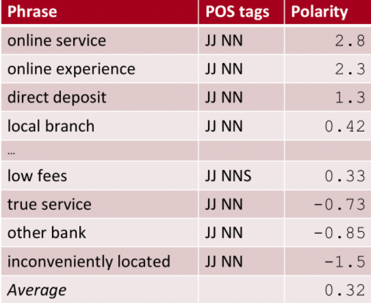
notice that
- “true service” has a low score, i.e. co-occur more often with negative word such as “poor”, hence indicative of bad reviews. The obvious one would be “inconveniently located”
- then the final score for the review will be the average. Here it is $0.32$, which means this review is slighltly positive.

Results from this algorithm on the Epinions dataset:

170 (41%) negative
240 (59%) positive
baseline (59%): guessing all positive
Turney algorithm: 74%

Note that again, this is good given that it is fully unsupervised!

Summary on Learning Lexicon

Both the algorithm covered above share the following pattern:

start with some seed set of words, e.g. “good”, “excellent”, “poor”
find other words that have similar polarity from some external dataset/search engine
- using “and” and “but”
- using co-occurance
add them to lexicon

Other Sentiment Task

Recall that:

Often sentiment analysis is framed as the detection of attitudes. In particular, we want to find out

Holder (source) of attitude
Target (aspect) of attitude
Type of attitude
- From a set of types: Like, love, hate, value, desire, etc.
- Or (more commonly) simple weighted polarity: positive, negative, neutral, together with strength
Text containing this attitude: which sentence/document

In reality:

Simplest task: Is the attitude of this text positive or negative? This will be our focus in this chapter as a classification task.
More complex: Rank the attitude of this text from 1 to 5, i.e. include strength
Advanced: all the 4 subtasks.

Here we discuss some approaches of identifying the target/aspect of a positive/negative review:

target: “The food was great but the service was awful”.

aspect: automatically find out it is talking about “food” and “service”

Finding Target/Aspect of a Sentiment

Some simple approaches for extracting aspects mentioned in some review:

rule-based: simple
1. find all frequenct phrases across reviews, e.g. “fish tacos”
2. filter again by some rules such as “an spect should occur after a sentiment word”. e.g. we need “… great fish tacos” to keep “fish tacos” unfiltered.
ML based: some aspects might not be in the sentence, i.e. its meaning is hidden. e.g. “… the place smells bad” correspond to something like “odor”.
1. hand-label a small corpus of reviews sentences with aspect, e.g. whether it is about “food, decor, service”, etc.
2. train a classifier on it

Then, once you have some way to extract aspect from a sentence, consider the following pipeline:

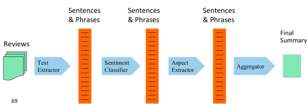
hence the general idea would be:

first do a sentence level sentiment classification
from the positive/negative reviews, extract the aspects using the trained classifier
hence obtain aspects level classifcation, essentially by combing the extracted aspect + whether if they are positive/negative from the sentence level

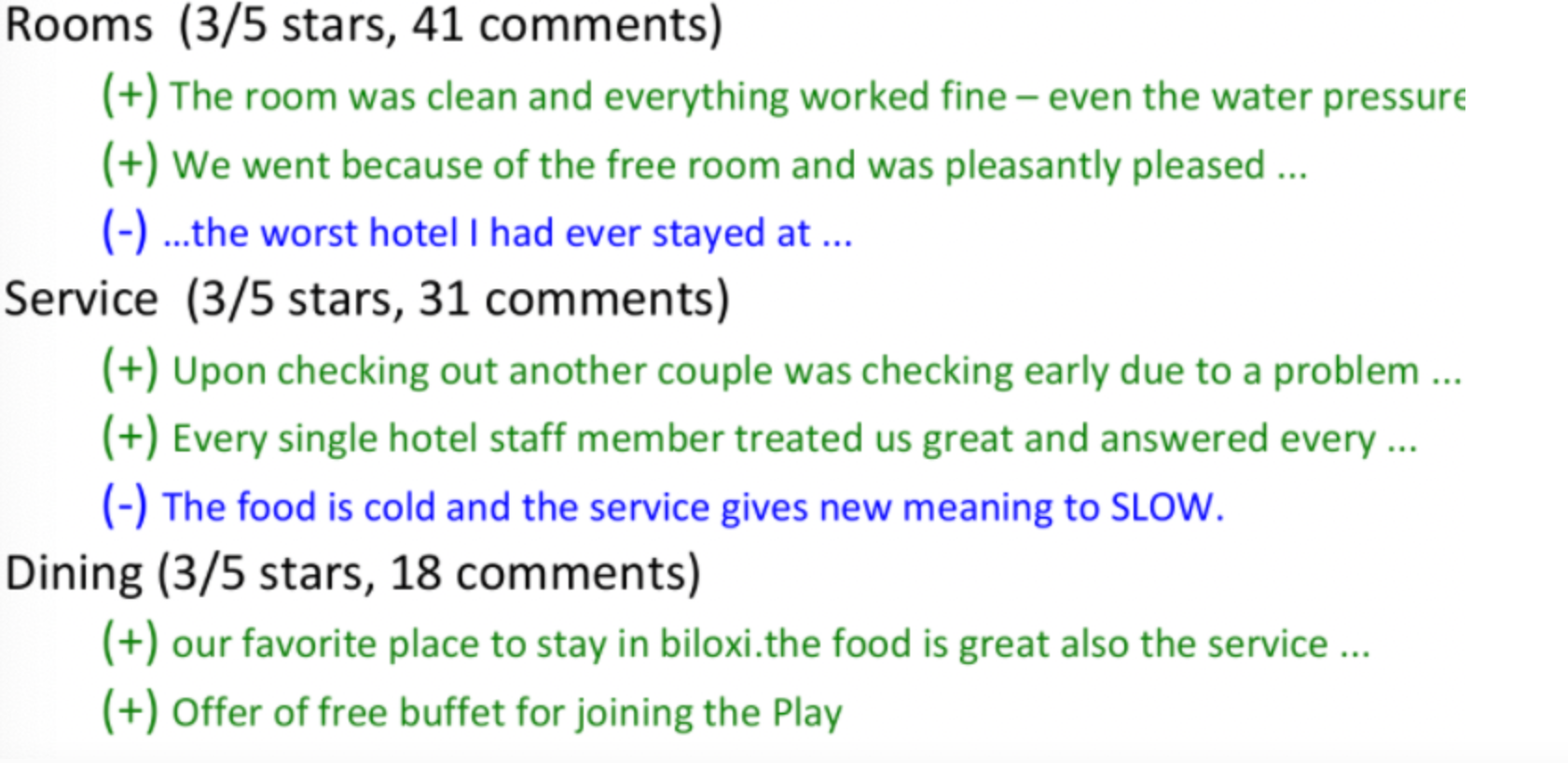
For Example, results would look like:

Explaining Sentiment Classification

Why is certain sentence clasified as positive/negative?

Still an active research topic, some current approaches:

we just highlight the words associated with positive/negative score
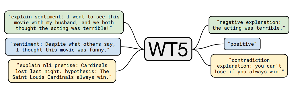
WT5, comes form T5. It is a text-to-text model, hene it can directly genrate a text explaining why it is a positive/negative post and classifying it

Summary on Sentiment Classification

Generally modeled as simple classification or regression task

predict a binary or ordinal label

Some common process/task/problems it involves:

how to deal with negation is important
Using all words (in naive bayes) works well for some tasks
\[c = \arg\max_{c_j \in C} P(W|c_j)P(c_j) =\arg\max_{c_j \in C} P(c_j)\prod_i P(w_i |c_j)\]
Finding subsets of words may help in other tasks
- Hand-built polarity lexicons
- Use seeds and semi-supervised learning to induce lexicons
A fully unsupervised approach such as Turney’s Algorithm

Statistical Significance Testing

In building systems we often need to compare the performance of two systems. How can we know if the new system we just built is better than our old one? How certain are we if one model performend better than nother on some test set?

Let us have:

two models we want to compare, model $A$ being the new one and $B$ being some baseline.
we are interested in testing on some metric $M$, such as $F_1$ score or accurarcy.
suppose we have some test set $x$ to evaluate on

Obviously we could measure:

\[\delta(x) = M(A,x) - M(B-x) \equiv \text{Effect Size}\]

for $M(A,x)$ is the performance of model $A$ on test set $x$ using metric $M$. Of course the larger the effect size the better, but another question we usually want to ask is:

if $A$’s superiority over $B$ is likely to hold again if we checked another test set $x’$

In the paradigm of statistical hypothesis testing, we test this by formalizing two hypotheses. Suppose you found $\delta(x)=0.2$, i.e. we have a $0.2$ higher e.g. accurarcy:

\[H_0: \text{what you observed is just a random effect}\\ H_1: \text{it is not random. Our model is better}\]

We want to show that $H_0$, the null hypothesis, has a low probability of happening, so that what we observed is not random/by chance:

\[\text{p-value}(x) \equiv P(\delta(X) \ge \delta(x) | H_0 \text{ is true})\]

i.e. we try on some random test set $X=x$ (with mean $0$) to get $\delta(x)$ again and again. If it is not by chance, then $\text{p-value}(x)$ should be small.

e.g. consider playing Poker, I claim that I am a better player, so the null hypothesis is that I win by luck.
then, suppose $\delta(x)$ is I win 10 “random” games in a roll. We know that $P(\delta(X) \ge \delta(x) \vert \text{I win by luck})$ is small. Hence I can reject the null hypothesis and conclude that I am actually a better player, if $\delta(x)$ happened.

Therefore, p-value gives the probability of observing a test statistic as extreme as the one observed $\delta(x)$, if the null hypothesis is true.

Hence, if the p-value is small, the observed test statistic is very unlikely under the null hypothesis

the expected value of $\delta(X)$ over many test sets, if assuming $A$ is not better than $B$ is $\mathbb{E}_X \delta(X) = 0$ for $X$ comes from a distribution with zero mean
how small should the p-value be? Often threshold such as $0.05,0.01$ is fine.

How do we compute the probability needed?

In NLP we generally don’t use parametric tests such as t-tests or ANOVAs as they make assumptions on the distributions of the test statistic (such as normality) that don’t generally hold in our cases So in NLP we usually use non-parametric tests based on sampling.

Either:

if we had lots of different random test sets $x^\prime$ with mean $0$ we could just measure all the $\delta(x^\prime)$ for all the $x^\prime$. This gives a distribution, from which we can compute probability of at least $\delta(x)$ happening if it is a random effect
use a bootstrap test by repeatedly drawing large numbers of smaller samples with replacement, under the assumption that the sample is representative of the population.

The Paired Bootstrap Test

The bootstrap test (Efron and Tibshirani, 1993) can apply to any metric; from precision, recall, or F1 to the BLEU metric used in machine translation.

The word bootstrapping refers to repeatedly drawing large numbers of smaller samples with replacement (called bootstrap samples) from an original larger sample.

in fact, the idea is to virtually create random test sets $X$ by sampling with replacement from a fixed test set $x$.

since this means we have $X$ with mean of $\delta(x)$, we would have to change the formula a bit

Consider a tiny text classification example with a test set $x$ of $10$ documents. And suppose we have $M$ being accuracy and we have two models $A$, and $B$:

where a slash means the model got it wrong. For this test set $x$, the effect size is $\delta(x)=0.2$.

We need to create a large distribution of test sets $X$. We can do this by:

pick a large number $b$, e.g. $b=10^5$ being the number of tests $x^{(i)}$ we want to create
each test $x^{(i)}$ will have $n=10$ same as $x$. Hence we repeatedly sample $n$ times from $x$ with replacement.
do until we created $x^{(b)}$

Now that we have the $b$ random test sets, providing a sampling distribution, we can compute how likely $A$ made $\delta(x)$ by pure chance. We might naively consider:

\[\text{p-value}(x) = \frac{1}{b} \sum_{i=1}^b \mathbb{1}\left( \delta(x^{(i)}) - \delta(x) \ge 0 \right)\]

so that if p-value is low, then $\delta(x)$ is not by pure chance. However, this would be wrong as

\[\text{p-value}(x) \equiv P(\delta(X) \ge \delta(x) | H_0 \text{ is true})\]

assumes the $X$ would yield a mean of $\delta(X)=0$. Here we would yield a $\delta(X=x)=0.2$ since it all came from the test set $x$.

Therefore, the correct one would be

\[\begin{align*} \text{p-value}(x) &= \frac{1}{b} \sum_{i=1}^b \mathbb{1}\left( \delta(x^{(i)}) - \delta(x) \ge \delta(x) \right)\\ &= \frac{1}{b} \sum_{i=1}^b \mathbb{1}\left( \delta(x^{(i)}) \ge 2\delta(x) \right) \end{align*}\]

So that if we have $10^5$ tests and for $47$ of them it happened that $\delta(x^{(i)}) \ge 2\delta(x)$, then it means p-value is $.0047$, i.e. it is very rare by chance. If we take a threshold of $0.01$ being significant, then we can say that this result $\delta(x)$ is statistically significant.

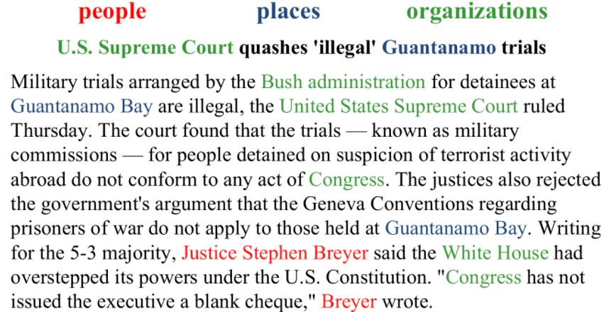
Information Extraction and NER

structed textual document: tables

Transform unstructured information in a corpus of documents or web pages into a structured data, e.g. populating a relational database, to enable further processing.

Consider receiving an email from job posting:

Raw Data/Email	Extracted Data

The task would be to extract information from some pre-defined attributes we want to extract.

i.e. givne the input, fill out the table (on the right) as much as we can
notice that each extracted info is an entity

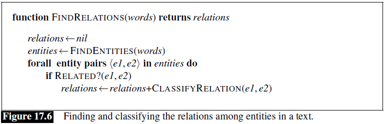
The general pipeline you want to consider is:

named entity recognition
relation extraction
template filling

Named Entity Recognition

Specific type of information extraction in which the goal is to extract formal names of particular types of entities such as people, places, organizations, etc.

Usually this is used as a preprocessing step for some future tasks, such as the template filling task we had, or question answering. Notice that this is a task in between sequence level and token level task - it is a span-oriented application.

Formally, given an input $x$ with $T$ tokens, $x_1,…,x_T$, a span is a continuous sequence of tokens with start $i$ and end $j$ such that $1 \le i \le j \le T$. Then in total for all possible span length we could have:

\[\frac{T(T-1)}{2}\]

total possible spans. Most application literally iterate through all possible spans. Hence they often have some application-specific length limit $L$ such that $j-i < L$ is required/legal span. We refer tot the set of legal span in $x$ as $S(x)$.

An example would be

Input	Output Desired

where note that we only find NER for the three entities we care here. Hence entities such as “Geneva Conventions” SHOULD NOT be highlighted. Hence this task is generally not easy.

In general, today we have two approaches:

train a BIO tagger. This will essentially be a Seq-labelling model
train an end-to-end model using GPT-3. This will be a Span-based Model

BIO-based NER

Some idea for training BIO-based model would be a Seq-labelling model

Training Data	BIO version of Training Data

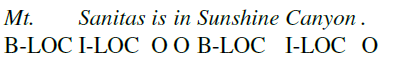Hence this is essentially a Seq-2-Seq decoding. A fuller example would be:

TODO: CRF on page 178-Chapter 8

Span-based NER

Some idea for training an end-to-end NN based model would be a span-oriented application.

generate representations for all the spans in the input. This often contains
- representations of the span boundaries, $h_i,h_j$ being the embeddings
- representation of the content in the span, $f(h_{i+1:j-1}) \to g_{ij}$
  - an example of such as function could be $f(h_{i+1:j-1}) = \bar{h}_{i+1:j-1}$ being the average
- combine the two representation, $\text{SpanRep}{ij} = [h_1;h_j;g{ij}]$
this can be done using contextualized input embeddings from the model
then, we have a span representation $g_{ij}$ for each span in $S(x)$. Then this is a classification problem where each span in an input is assigned a class label $y$:
\[y_{ij} = \text{softmax}(\text{FFNN}(\text{SpanRep}_{ij})) \in \mathbb{R^{|Y|}}\]
since most spans will not have a label, we add $y = \text{null} \cup y$ to the set of labels, and hence $\vert Y\vert =\vert y\vert +1$.
then for decoding, take $\arg\max y_{ij}$ to get the tag.

Note that some post-processing steps will need to be done to prevent overlapping classifications, as this scores all $T(T-1)/2$ spans. However, it does have a benefit as it naturally accommodate embedded named entities:

e.g. both “United Airlines” and “United Airlines Holding” would be evaluated

a BIO based tagging approach would have not looked at this.

A detailed example would be:

instead of taking average, we consider using the embeddings as
\[g_{ij} = \text{SelfAttn}(h_{i:j})\]
so that the representation would be centered around the head of the phrase corresponding to the span. Then combining to get:
\[\text{SpanRep}_{ij} = [h_1;h_j;g_{ij}]\]
finally doing the same:
\[y_{ij} = \text{softmax}(\text{FFNN}(\text{SpanRep}_{ij}))\]

Hence graphically

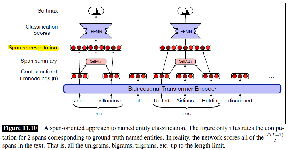
where:

cross-entropy loss would be used

Relation Extraction

Now we have detected named entities, our next step is to discern relationships between those entities. For instance:

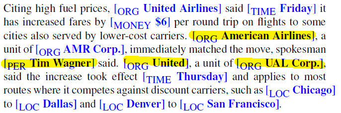
where form the highlighted part, we know that:

“Tim Wagner” is a spokesman for “American Airlines”
“United” is a unit of “UAL Corp”
etc.

All of those are simple binary relationships which fall under some generic categorization such as:

basic 3 relations: employed-by; located-at; part-of
a more complicated 17 relations used in ACE relation extraction

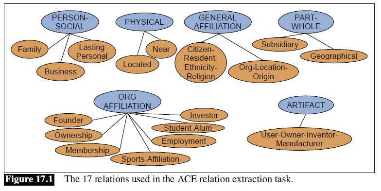
Hence, a graphical representation of what are doing now is:

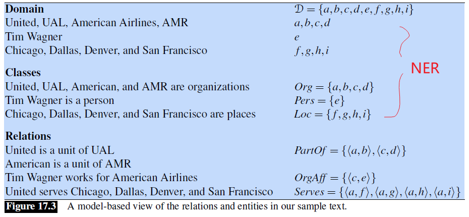
where:

the first two steps can be done in a NER
the relation can be seen as consisting of a set of ordered tuples over elements of a domain (e.g. named entities)

Relation Extraction Algorithms

Now, we answer the question: how do we find those relations? In general, there are four main ways to do it

handwritten patterns
supervised machine learning
semi-supervised (via bootstrapping or distant supervision)
unsupervised

Using Patterns to Extract Relations

Consider the example of:

where we notice that “Gelidium” is a hyponym of “red algae”, which can be identified using the following pattern

\[NP_0 \text{ such as } NP_1 \{,NP_2,...,(\text{and,or})NP_i\}\]

implies the relation

\[\forall NP_i,i\ge 1, \text{hyponym}(NP_i, NP_0)\]

which inspires pattern such as

Pattern	Example

but of course, with hand-crafted rules we have:

advantage of high precision as they are tailored to specific domains
low recall, missing a lot
not scalable

Relation Extraction via Supervised Learning

Consider now having the

input of: a fixed set of entities
label of: a fixed set of pre-defined relations

Then approaches to make it a classification problem could be: for each possible pair, apply a multiclass classification for each class being the relation

where the feature/embeddings of the named entity $e_1,e_2$ could be:

word level embeddings of the named entity $e_i$
head word embedding of the named entity
encoding the named entity’s type, e.g. if it is ORG, or PER
number of entities in this sentence
encoding some syntactic structure of the sentence
etc

then the architecture of the classifier could be

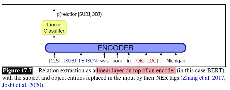
where notice that

essentially using a transformer, hence using context embeddings for the content
we also included the entire sentence to give context for the two named entities in this case

of course, this can be optimized as we can skip some pairs for certain relation as it won’t happen at at all

But labeling a large training set is extremely expensive and supervised models are brittle: they don’t generalize well to different text genres.

For this reason, much research in relation extraction has focused on the semi-supervised and unsupervised approaches we turn to next.

other problem include: what if the relation set is not fixed? Then of course supervised version would not work.

Semi-supervised Relation Extraction

One idea is to bootstrap more relation-labeled entity pairs from some known small sample labelled pair. For instance, suppose you want to get a relation being airline/hub pair, and you already have

\[\text{Ryanair has a hub at Charleroi} \iff \text{[ORG] has a hub at [LOC]}\]

being a known pair, you can:

finding other mentions of this relation in our corpus
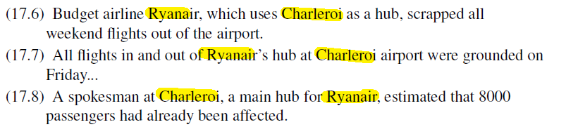
use features such as context to extract general patterns such as the following

which signifies a “rule” for airline/hub pair
use these new patterns can then be used to search for additional tuples.
assign confidence values to new tuples, and add to the dataset if high confidence
- this is to avoid semantic drift. In semantic drift, an erroneous pattern leads to the introduction of erroneous tuples, which, in turn, lead to the creation of problematic patterns and the meaning of the extracted relations ‘drifts’.

Hence, given some seed samples that have relation $R$, we can populate this set by

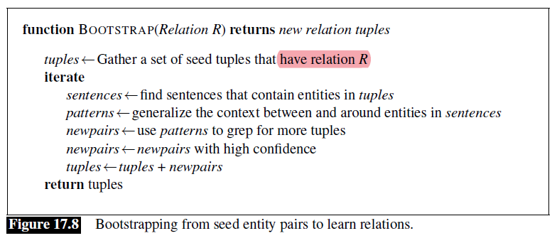
Once done, apply supervised classification as mentioned above.

Unsupervised Relation Extraction

The goal of unsupervised relation extraction is to extract relations from the web when we have no labeled training data, and not even any list of relations.

This task is often called open information extraction or Open IE.

For example, the ReVerb system (Fader et al., 2011) extracts a relation from a sentence s in 4 steps:

Run a part-of-speech tagger and entity chunker over $s$
For each verb in $s$, find the longest sequence of words $w$ that start with a verb and satisfy syntactic and lexical constraints, merging adjacent matches.
For each phrase $w$, find the nearest noun phrase $x$ to the left which is not a relative pronoun, wh-word or existential “there”. Find the nearest noun phrase $y$ to the right.
Assign confidence $c$ to the relation $r = (x;w;y)$ using a confidence classifier and return it.

Template Filling

Task: fill the slots in the associated templates with fillers extracted from the text.

those fillers could come from text segments extracted directly from the text

consist of concepts that have been inferred from text elements through some additional processing

A template looks like

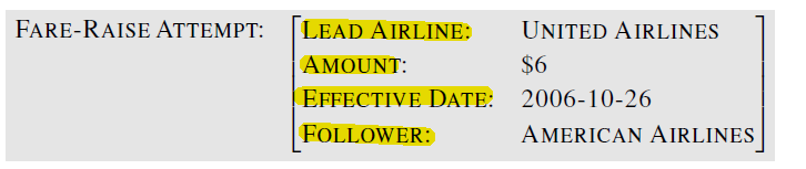
where we have four slots.

The next section describes a standard sequence-labeling approach to filling slots.

Supervised Approach to Template Filling

We are given

training documents with text spans annotated with predefined templates and their slot fillers.
note that there can be multiple different templates

Our goal is to

create one template for each event in the input
fill in the slots with text spans.

Hence this means that we can split the task to train two classifiers

first system decides whether the template is present in a particular sentence
- called template recognition or event recognition
Then the
- input could be a sequence of words, with the usual set of features can be used: tokens, embeddings, word shapes, part-of-speech tags, syntactic chunk tags, and named entity tags.
- output is indicating any slot from a template being detected
Then if detected, feed that sequence of words into the second system with that detected template
second system has the job of role-filler extraction.
- for each role in the template, e.g. LEAD-AIRLINE, AMOUNT, etc
- train a binary classifier that on each possible span to decide if it would fill in the blank
However, this means that you would need to resolve conflicts as multiple non-identical text segments could be labeled for the same slot.

IE Examples

below contains examples over some typical datasets you would deal with.

MUC

Message Understanding Conference (MUC) was an annual event/competition where results were presented.

But since this is found by DARPA, it cares more about military related. Focused on extracting information from news articles:

Terrorist events
Industrial joint ventures
Company management changes

Medline Corpus

Contains medical related data

Input	NER: Proteins

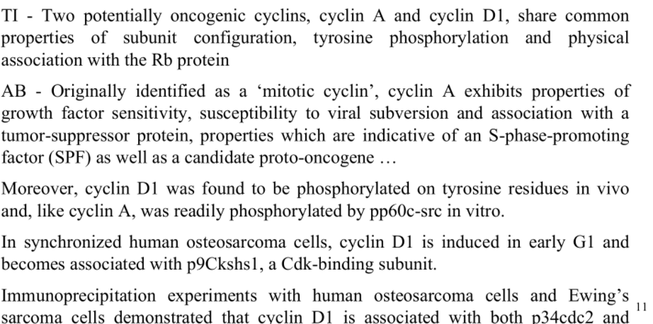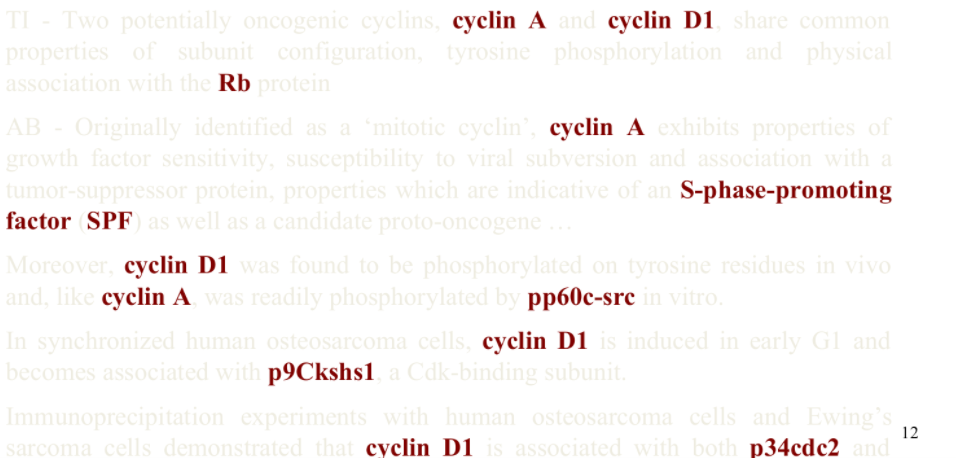Web Extraction

Another example would be web extraction

because those dynamically webpages generally reads data from database, it is often a semi-structured data
i.e., we want to view the webpage back as a structured table/database. An extractor for this case is often called a wrapper

An example would be the Amazon Book Descriptions pages:

Input Information	Extracted Information

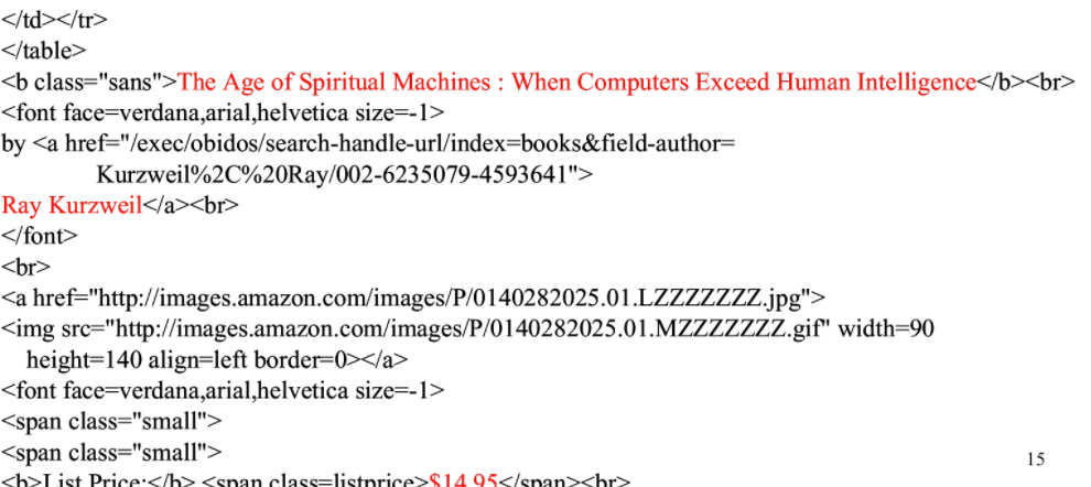where note that here:

the template could be learnt as well
since it is from HTML, we could image many rule-based approach works equally well

e.g. using Enhanced REGEX including

\b for word boundary
\d for a digit
{} repetition operator, e.g. A{1,5} means you can have one-to-five A

Some examples include (in Perl):

/\b($\d{3}$\s?)?\d{3}-\d{4}\b/ for US phone number

Hence for filling in each field:

Price pattern: \b\$\d+(\.\d{2})?\b. However, we also need to to identify proper context.
- Pre-filler pattern: <b>List Price:</b> <span class=listprice>
- Post-filler pattern: </span>
those could also be induced, e.g by RAPIER
of course, for other non-html format, REGEX may not work as well hence you need to train classifiers

Evaluating IE Accuracy

Consider we have a fixed template to begin with, which has $N$ slots. Then:

our model extracted $C$ correct slot/value pairs in the template
extracted a total number of $E$ pairs

Then we can apply

precision=$C/N$
recall=$C/E$
$F_1$ measure from the above

Question Answering

The goal of question answering is to build systems that automatically answer questions posed by humans in a natural language

Most question answering systems focus on a particular subset of these information needs: factoid questions, questions that can be answered with simple facts expressed in short texts:

e.g. “Where is the Louvre Museum located?”

In general, the two common paradigms that solve this task are

Information-retrieval (IR) based QA, sometimes called open domain QA, which relies on the vast amount of text on the web:
1. Given a user question, perform pre-processing of the question including tokenization/normalization
2. information retrieval is used to find relevant passages, i.e. find documents that contain an answer
  - using cosine similarity of some vector representation of the query and documents you have
3. Then neural reading comprehension algorithms read these retrieved passages
4. Draw the answer as a span of text from the passage (like SAT, GRE exams)
knowledge-based question answering, which
1. builds a semantic representation of the query
2. These meaning representations are then used to query databases of facts

Bonus: for large pretrained language models (i.e. on next word prediction), they can sometimes directly answer the question. This work because huge pretrained language models have already encoded a lot of factoids

Information Retrieval

Information retrieval or IR is the name of the field encompassing the retrieval of all manner of media based on user information needs. The resulting IR system is often called a search engine.

In particular, the IR we consider is called ad hoc retrieval, which:

a user poses a query to a retrieval system
we output an ordered set of documents from some collection

where:

A document refers to whatever unit of text the system indexes and retrieves (web pages, scientific papers, etc)
A term refers to a word in a collection, but it may also include phrases
the vector hence can be a TF-IDF vector or a bag of words. Then we can measure similarity for ranking.

Term weighting and document scoring

Recall that if we use TF-IDF

TF-IDF essentially consist of two components:

term frequency in log, essentially captures the frequency of words occurring in a document (i.e. the word-document matrix)

inverse document frequency, essentially giving a higher weight to words that occur only in a few documents (i.e. they would carry important discriminative meanings)

The term frequency in a document $d$ is computed by:

\[\text{tf}(t,d) = \log_{10}(\text{count}(t,d) + 1)\]

where:

we added $1$ so that we won’t do $\log 0$, which is negative infinity

The document frequency of a term $t$ is the number of documents it occurs in.

note that this is different from collection frequency of a term, which is the total number of times the word appears in any document of the whole collection

For example: consider in the collection of Shakespeare’s 37 plays the two words Romeo and action

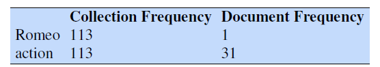
Therefore, we want to emphasize discriminative words like Romeo via the inverse document frequency or IDF term weight:

\[\text{idf}(t) = \log_{10}\left( \frac{N}{\text{df}(t) } \right)\]

where:

apparently $\text{df(t)}$ is the number of documents in which term $t$ occurs and $N$ is the total number of documents in the collection
so essentially, the fewer documents in which a term occurs, the higher this weight.
notice that we don’t need $+1$ here because the minimum document frequency of a word in your corpus would be $1$
again, because the number could be large, we use a $\log$.

Here are some IDF values for some words in the Shakespeare corpus

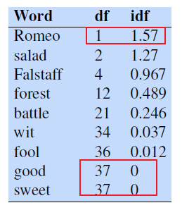
Finally, the TF-IDF basically then does:

\[\text{TF-IDF}(t,d) = \text{tf}(t,d) \times \text{idf}(t)\]

An example would be:

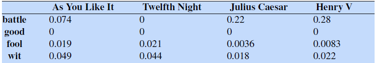
where notice that:

essentially it is still a term-document matrix, but it is weighted by IDF.
notice that because $\text{idf(good)}=0$, the row vector for good becomes all zero: this word appears in every document, the tf-idf weighting leads it to be ignored (as it is not very informative anymore)

Document Scoring

Then, the above provide a way to represent a document by a vector (vertically). Then essentially:

encode document $d$ to vector $\vec{d}$
encode query $q$ to vector $\vec{q}$
measure similarity as score:
\[\text{score}(q,d) = \cos (\vec{q},\vec{d}) = \frac{\vec{q}\cdot \vec{d}}{|\vec{q}||\vec{d}|}\]

However, since most queries are short and contain unique words, we want to approximate this by:

\[\begin{align*} \text{score}(q,d) &= \frac{\vec{q}}{|\vec{q}|}\frac{\vec{d}}{|\vec{d}|}\\ &= \sum_{t \in q} \frac{\text{tf-idf}(t,q)}{\sqrt{\sum_{t'\in q}\text{tf-idf}(t',q)^2}} \cdot \frac{\text{tf-idf}(t,d)}{\sqrt{\sum_{t'\in d}\text{tf-idf}(t',d)^2}}\\ &\approx \sum_{t \in q} \frac{\text{tf-idf}(t,d)}{\sqrt{\sum_{t'\in d}\text{tf-idf}(t',d)^2}}\\ &= \sum_{t \in q} \frac{\text{tf-idf}(t,d)}{|\vec{d}|} \end{align*}\]

where the third approximation comes from:

since we assume sparse query and unique words, hence
\[\text{TF-IDF}(t,q) = \text{tf}(t,q) \times \text{idf}(t)\approx \text{idf}(t)\]
as term frequency is approximately one
then the inverse document frequencies will be a constant for each document $d$, hence $\vert \vec{q}\vert$ will not affect ranking

For Example: Consider utilizing the above to rank the following query/document

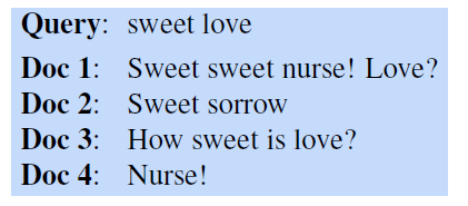
then, we first compute the TF-IDF like a term-document matrix

where as an example, we see that document 2 which is “Sweet sorrow” has:

term frequency of only those two words appearing once, then TF is computed by
\[\text{tf}(t,d) = \log_{10}(\text{count}(t,d) + 1)=\log_{10}(1+1) = \log_{10}(2)\]
for both word
document frequency of “sweet” appears in three of the collection of documents, and “sorrow” only appeared here hence a count of one.

Finally, we use this forumula to compute similarity by iterating through words in the query

\[\sum_{t \in q} \frac{\text{tf-idf}(t,d)}{|d|}\]

which basically iterates over the word “sweet” and then “love”, hence we get:

Note that in this formula, if document $d$ contains none of the words in query $q$, then it will have a score of zero. This is why we needed the inverted index to quickly filter documents and only get the ones containing terms in $q$.

In the previous example, we have included preprocessing steps such as:

remove punctuations and convert to lower case
(deprecated) remove high-frequency words (e.g. stop words) from both the query and document before representing them

where the latter is no longer used as it is partly handled by the TF-IDF weighting already and it could make query such as “to be or not to be” to be reduced to “not”, which makes IR hard.

Inverted Index

As mentioned before, In order to compute scores, we need to efficiently find documents that contain words in the query.

The basic search problem in IR is thus to find all documents $d \in C$ a collection that contain a term $q\in Q$ a query.

An inverted index basically maps each word to indices of documents $d$ that contains the word. For instance, consider the same example as before

Text	Example TF-IDF

The idea is to establish an index of all words in our database, and we get

where:

each word containing its document frequency in ${}$, which is the same as the ones computed in previous example
a pointer to a postings list that contains document IDs and term counts in $[]$.
- e.g. the word “nurse” appeared in document ID 1 and 4, each once.

Then, with this structure, we can:

given a list of terms in query
very efficiently get lists of all candidate documents and together with the TF and DF values, hence easily compute the scores.

IR with Dense Vectors

The score and hence collection of document returned using TF-IDF heavily depended us to have overlapping words in the document.

In other words, the user posing a query (or asking a question) needs to guess exactly what words the writer of the answer might have used to discuss the issue.

e.g. we want to search for “tragic love story” but Shakespeare writes instead about “star-crossed lovers”.

This is called the vocabulary mismatch problem

Therefore, the solution is to find a representation that can handle synonymy: instead of (sparse) word-count vectors, using (dense) embeddings, e.g. encoders like BERT.

In fact, in what is sometimes called a bi-encoder we use two separate encoder models $\text{BERT}_Q, \text{BERT}_D$:

one to encode the query $q$
\[h_q = \text{BERT}_Q(q)[\text{CLS}]\]
where since we need a single vector, we take the embedding of the $[\text{CLS}]$ token which encodes all information of the sequence
one to encode the document $d$
\[h_d = \text{BERT}_D(d)[\text{CLS}]\]
use the dot product between these two vectors as the score
\[\text{score}(d,q) = h_d \cdot h_q\]

Hence graphically

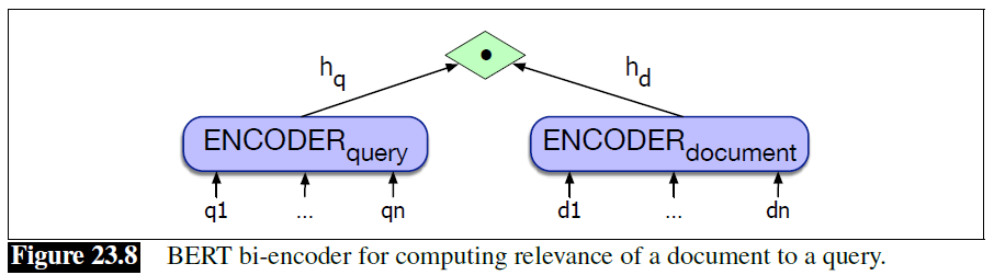
Some challenges in this area is:

Among the many areas of active research are how to do the fine-tuning of the encoder modules on the IR task
Efficiency is also an issue. For TF-IDF version we had inverted index which allowed us to quickly rank documents. But here, with dense vectors we need a Nearest Neighbor search, which is inefficient.
- Modern systems therefore make use of approximate nearest neighbor vector search algorithms like Faiss

IR-Based Factoid QA

Finally, we come back to how to perform QA task using IR.

The goal of IR-based QA (sometimes called open domain QA) is to answer a user’s question by

finding a related document among the web or some other large collection of documents. (IR task)

finding short text segments from the selected related documents (what we are doing here)

Some examples of what we need to do include:

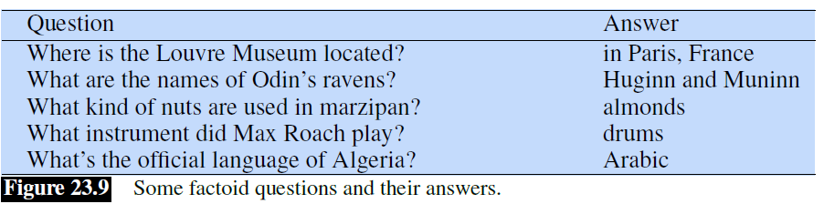
Therefore the dominant paradigm implementation basically includes two steps:

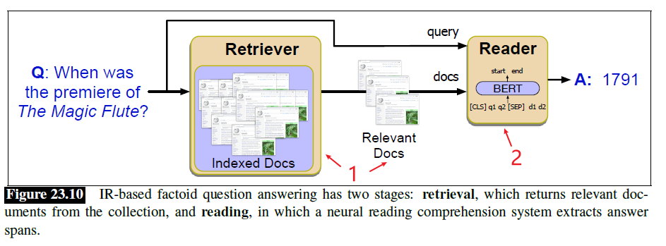
which is essentially a retrieve and read model

use retriever to retrieve relevant passages from a text collection, usually using a search engines
- this we have discussed before in IR, e.g. use Dense Vectors for embedding
a neural reading comprehension algorithm passes over each passage and finds spans that are likely to answer the question
- given the query $q$ and a sample passage $p$ that could contain the answer
- return an answer $s$ or perhaps declare there is no answer
- hence here it becomes a close domain QA as we only have a fixed set of selected documents to look at

For the above to work, we will need a few components in the pipeline (we have already discussed the retriever in IR):

datasets for reading comprehension
how to make a neural reader

IR-based QA: Datasets

Our aim is to train a reading comprehension systems, so that given a passage and a question, and predicts a span in the passage as the answer. Therefore, we consider comprehension datasets containing tuples of (passage, question, answer).

Stanford Question Answering Dataset (SQuAD), consists of passages from Wikipedia and associated questions whose answers are spans from the passage
Squad 2.0 in addition adds some questions that are designed to be unanswerable

Examples look like:

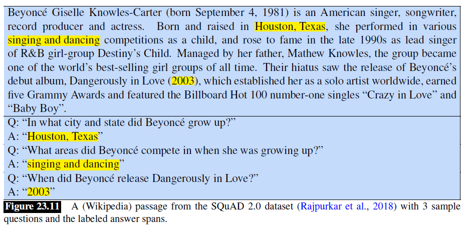
However, those datasets are often constructed by having annotators first read the passage, then construct QAs. This could make the questions easier. Hence, we also attempted to make datasets from questions that were not written with a passage in mind.

TriviaQA dataset resulting in 650K question-answer-evidence triples
etc.

IR-based QA: Reader

The retriever have now found a couple of relevant documents. Hence

The reader’s job is to take a passage and a question as input and produce the answer.

In the extractive QA we discuss here, the answer is a span of text in the passage

(skipped )more difficult task of abstractive QA, in which the system can write an answer which is not drawn exactly from the passage.

For example:

given a question like “How tall is Mt. Everest?” and a passage that contains the clause “Reaching 29,029 feet at its summit, a reader will output 29,029 feet.”
output “29,029 feet.”

Then this is a span-labelling task (e.g. Span-based NER), i.e. we output a span that we think constitutes the answer

given a question $q$ of $n$ tokens, $q_1,…,q_n$, and a passage $p$ of $m$ tokens that could contain the answer $p_1,…,p_m$

return $p(a\vert q,p)$ for each span $a \in S(p)$ a set of possible spans in $p$

Alike NER, we would need to score all possible spans, but we can make a assumption/simplification that

\[P(a|q,p) = P_{start}(a_s|q,p)P_{end}(a_e|q,p)\]

for basically $P_{start}(i\vert q,p)$ means token $p_i$ is the start of the span, and similarly for $P_{end}(j\vert q,p)$. How do we model such a probability? A standard baseline would be using BERT

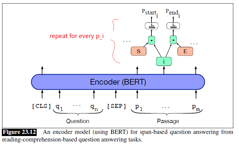
where:

since we are conditioned on $q,p$, we pass both as input to the encoder
we add two new special vectors: a span-start embedding $S$ and a span-end embedding $E$, which will be learned in fine-tuning so that
\[P_{start}(i|q,p) = \text{Softmax}(S \cdot \vec{p}_i') = \frac{\exp(S \cdot \vec{p}_i')}{\sum_j \exp(S \cdot \vec{p}_j')}\]
where the embedding vector $\vec{p}_i’$ of token $p_i$ would have already contained information from $q$. Similarly
\[P_{end}(i|q,p) = \text{Softmax}(E \cdot \vec{p}_i') = \frac{\exp(E \cdot \vec{p}_i')}{\sum_j \exp(E \cdot \vec{p}_j')}\]
then, the training objective would be maximizing the probability of correct start and end positions, hence minimizing negative log likelihood:
\[L = -\log P_{start}(i^*|q,p) - \log P_{end}(j^*|q,p)\]
where $i^, j^$ are the gold labels.
for inference, we output the highest $\arg\max_{i,j} P_{start}(i\vert q,p)P_{end}(j\vert q,p)$ ** which is the same as finding the **highest score of
\[\arg\max_{i,j} P_{start}(i|q,p)P_{end}(j|q,p) = \arg\max_{i,j} S \cdot \vec{p}_i' + E \cdot \vec{p}_j'\]
as products of the exponentials (from the Softmax) are basically comparing sums of exponents

Other model prior to BERT include BiDAF, Bidirectional Attention Flow model:

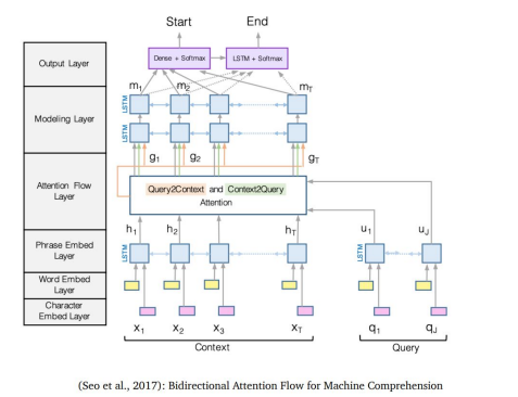
where the output is the same, $i,j$, but here the major difference is that

attention: query to context attention, i.e. $q\to d$, and context to query attention, i.e. $d \to q$

C2Q Q2C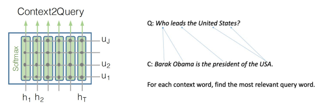

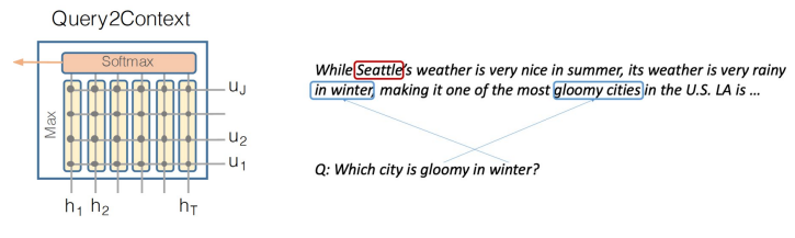
so that:
- Context-to-query attention: For each context word, choose the most relevant words from the query words.
- Query-to-context attention: choose the context words that are most relevant to one of query words.
modelling: uses Bidirectional LSTM for encoding, which is sequential and hence not efficient. So, its speed is suboptimal compared to Transformer based which suitable for parallelization.

Knowledge-based QA

Knowledge-based question answering: the idea of answering a natural language question by mapping it to a query over a structured database.

Two common paradigms are used for knowledge-based QA.

graph-based QA, models the knowledge base as a graph, i.e. entities as nodes and relations or propositions as edges between nodes.
QA by semantic parsing, using the semantic parsing methods

Both of the methods above would need some entity linking step. Hence this will be discussed first.

Entity Linking

Entity linking is the task of associating a mention in text with the representation of some real-world entity in an ontology.

The most common ontology for factoid question-answering is Wikipedia, since Wikipedia is often the source of the text that answers the question

For example,

given the sentence “Paris is the capital of France”
the idea is to determine that “Paris” refers to the city of Paris and not to Paris Hilton or any other entity that could be referred to as “Paris”.

In many practical cases, the set of entities will be the set of Wikipedia articles, where each article itself is an unique entity.

skipped, but can be treated as a sequence labelling task and use NN based methods

Knowledge-Based QA from RDF stores

Here we focus on the very simplest case of graph-based QA, in which the dataset is a set of factoids in the form of RDF triples

RDF triple is a 3-tuple, a predicate with two arguments, expressing some simple relation or proposition. An example would look like

Then, we can use this by:

locate the entity asked in the query $Q$

check which relation is it asking, e.g. birth-year?

return the answer in this RDF triplet

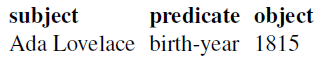
Let’s assume we’ve already done the stage of entity linking introduced in the prior section. Thus we’ve mapped already from a textual mention like Ada Lovelace to the canonical entity ID in the knowledge base. Then:

determine which relation is being asked about. e.g.
\[\text{“When was ... born”} \to \text{"birth-year"}\]
so that the question becomes:
\[\text{“When was Ada Lovelace born?”} \to \text{birth-year (Ada Lovelace, ?x)}\]
For simple questions, where we assume the question has only a single relation, relation detection and linking can be done in a way resembling the neural entity linking models: computing similarity (generally by dot product) between the encoding of the question text and an encoding for each possible relation.
then, once we located the relation like above, return the answer by fetching in the RDF database

Knowledge-Based QA by Semantic Parsing

The second kind of knowledge-based QA uses a semantic parser to map the question to a structured program to produce an answer.

basically into a query language like SQL or SPARQL

Examples of input question and output formatted query looks like:

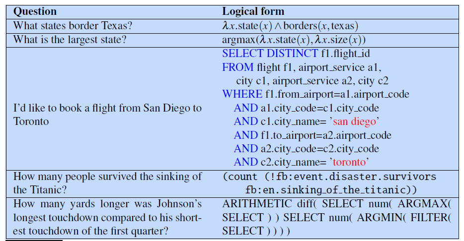
where the logical form of the question is thus either in the form of a query or can easily be converted into one (predicate calculus can be converted to SQL, for example).

In a supervised case, the task is then to take those pairs of training tuples (question and logical form pair) and produce a system that maps from new questions to their logical forms.

A common baseline algorithm is a simple sequence-to-sequence model, for example using BERT:

using BERT to represent question tokens
passing them to an encoder-decoder

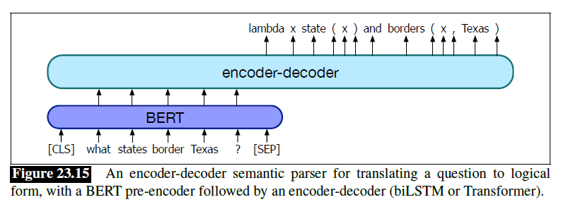
Recall: Encoder-Decoder

Essentially for decode, we usually do it auto-regressively so that suppose our decoder has Attention with MAX_SEQ_LEN=32. Then:

the input to decoder done auto-regressively:

at $t=0$, there is no input/or we have <pad><pad>...<s> for filling the 32 sequence length and a positional embedding
get cross attention from encoder output
generate an output “I” and feed back as input at $t=1$. So we get <pad><pad>...<s>I as the input of decoder
repeat until </s> is generated

Note: Comparing with using a RNN based decoder, when we are generating output $o_{t+1}$, the difference is:

transformer based can only condition/read in $o_{t-31},…,o_t$ for a max sequence length of 32 for the attention layer

RNN based can use $h_t$ which encodes all previous information. However, it has no attention/is sequential.

Essentially it is a Seq-2-Seq architecture, hence often done auto-regressively.

Using Language Models

An alternative approach to doing QA is to query a pretrained language model, forcing a model to answer a question solely from information stored in its parameters.

The popular model in this case is the T5 language model, which is

an encoder-decoder architecture (mentioned above)
pretrained to fill in masked spans of task

The general picture of what it does is

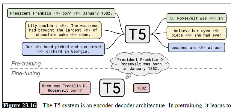
where as it is trained as a language model, we needed to finetune the T5 system to the question answering task, by giving it a question, and training it to output the answer text in the decoder.

Evaluation of Factoid Answers

Factoid question answering is commonly evaluated using mean reciprocal rank, or MRR

MRR is designed for systems that return a short ranked list of answers or passages for each test set question, so that:

each test set question is scored with the reciprocal of the rank of the first correct answer

then MRR is the average of the scores for each question in the test set

For example, if the system returned

five answers to a question (with its own ranking)
but the first three are wrong (so the highest-ranked correct answer is ranked fourth)

Then the reciprocal rank for that question is $1/4$. (The score for questions that return no correct answer is $0$.)

Therefore, more formally, for a system returning ranked answers to each question in test set $Q$, then MRR is

\[\text{MRR} = \frac{1}{|Q|} \sum_{i=1}^{|Q|} \frac{1}{\text{rank}_i}\]

On the other hand, reading comprehension systems on datasets like SQuAD are evaluated by:

Exact match: The % of predicted answers that match the gold answer exactly
F1 score: The average word/token overlap between predicted and gold answers.
1. Treat the prediction and gold as a bag of tokens,
2. compute F1 for each question
3. return the average F1 over all questions.

Language Generation

Text generation is a subfield of natural language processing (NLP). It leverages knowledge in computational linguistics and artificial intelligence to automatically generate natural language texts

Typically, you will see architectures generating a text be:

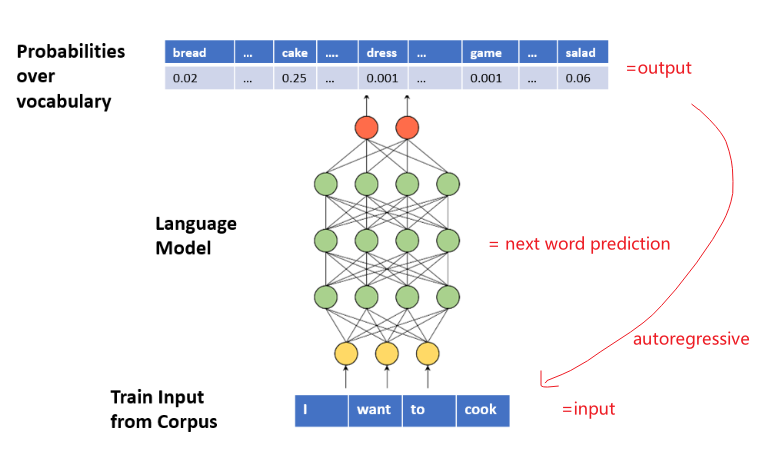
where essentially:

the language model’s aim is to output a distribution for next word $w_{n+1}$, given the input $w_1,..,w_n$
hence essentially it is outputting $P(w_{n+1}\vert w_{i},…,w_n)$, hence called the language model
this is usually done in an auto-regressive way, i.e. generated output is fed back as input until we generated some end of sentence token, such as </s>.
this architecture is related to many down stream tasks such as Machine Translation, Dialog Generation, etc.

E2E Challenge

Here, we will discuss an example application, which is the E2E challenge:

domain: restaurant recommendation
task: we want to generate texts (one or more sentences) to recommend restaurants from an input meaning representation (MR)

An example of meaning representation include

Example MR	Labelled

where essentially your output should fulfill the above requirement specified in the MR.

dialogue act: in this competition, request or inform (here we only have two)
attributes/values: unordered attributes of the generated text that you need to fulfill (all those attributes needs to be mentioned) this will be a fixed set, which is called domain ontology:

so in this task, there will only be 8 types.

An example output that fulfills the about MR would be

E2E Datasets

Finally, before we discuss how to construct a model, it is important to know how training data is collected:

Crowd sourcing on CrowdFlower (similar to Amazon Mechanical Turk)
essentially it asks you to generate the text given the MR (either in a pure text format or pictorial)

An example would be

Pictorial	Text MR	Sample Training Text

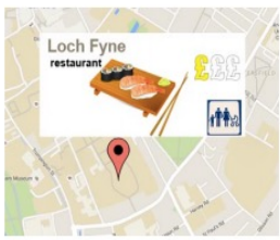why did we also provided a pictorial representation to the CrowdFlower works?

The aim is to generate good training text from human workers.
it turs out that they generate better texts if a picture is provided.

Then, you get training dataset:

6K MRs with average of 8.27 texts per MR
5 slots (attribute-key pairs) per MR

Text Generation Modelling

Traditionally, for conditional text generation tasks, you will need to consider

Content selection (Done for us as MR in the E2E task)
Aggregation: which pieces of content go into which sentence? e.g. generate abstract syntax tree from selected content
Realization: tree to real sentence

Which results in two paradigms:

Two step generation: first find a sentence planning. Then, given a plan, realize it into natural language.
Joint one-step approach: usually use Seq-2-Seq model, where input sequence would be a string of the requirements (e.g. MR)

For example:

Input MR	Input MR into Tree	Realization

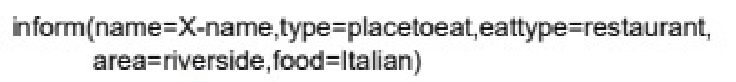Generating using Seq-2-Seq

This is often the architecture used today, where we essentially have:

encode the input MR as as string
- either make it a sequence of triples (Dialogue Act, Slot, Value), so that you could get input like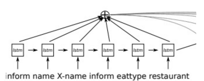
- or find a syntax tree and then use the string flattened version of the tree
  
  Tree String Version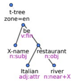
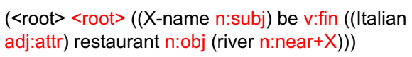
input the above string
output generated text

Then, the Seq-2-Seq model basically does

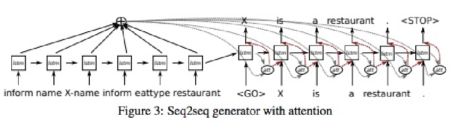
which is basically a auto-regressive generation.

of course, you could also replace LSTM blocks with transformers
the output at each state is essentially $P(y_{t}\vert y_1,…,y_{t-1},h_x)$ where $y_i$ are the generated ones and $h_x$ is the hidden state representation of the input sequence. Here we are only outputting the single best word at a time, hence
\[o_t = \arg\max_y P(y_{t}|y_1,...,y_{t-1},h_x)\]
but remember this is a greedy search. In reality you can use beam search to allow for keeping more than one options.

Problems with Seq-2-Seq

But, as we are using NN, there are some bigger problems. We will not be able to enforce constraints such as

Missing to fulfill an attribute
Added an attribute/value that did not exist in MR
Wrong value for an attribute (hallucination).

For instance: the red parts are the wrong values not mentioned in the MR

Input MR	Seq-2-Seq output with Beam Search of width 3

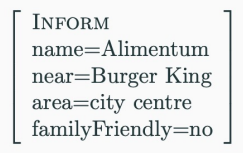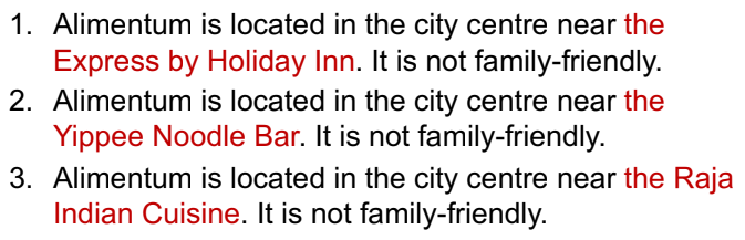some intuition of why, instead of Burger King, we get those random place names:

essentially the network learns some hidden representation of the words in the MR. So suppose we have the following training data

| | | | :———————————————————-: | :———————————————————-: |

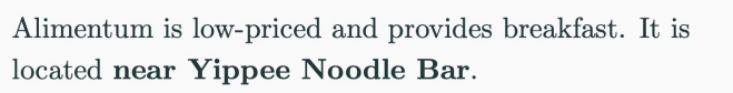then the model would have learnt a similar vector representation between “Burger King” and “Yippee Noodle Bar”
then as what the models see are representations of “Burger King”, it is likely that “Yippee Noodle Bar” could be outputted

How do we deal with those problems?

Missing/Added value: use a Re-ranker, which is an additionally penalty using hamming distance

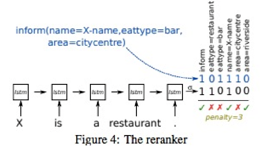
where the sequence 110100 will be the output of an additional classifier (which we hope is doing the correct job)
- it is called reranker as it adds the penalty and reranks the output
- since we need to rank outputs, we would use a beam search
- of course, this does not solve the problem entirely, but does help a bit
Wrong Value: using data augmentation techniques - faithful speaker

Results

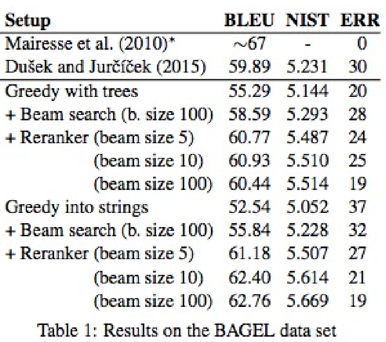
where we see:

re-ranked + beam search does better than raw beam search
raw string input does better than tree as it has more flexibilities.

However, on many hard constraint tasks, seq2seq often fail to correctly express a meaning representation hence can be outperformed by hand-engineered solutions. But the key advantage is that it is much less costly in time and money.

E2E Data Augmentation

Here, we discuss how to use data augmentation to solve the wrong value problem. We will discuss two approaches:

delexicalization: simplest data augmentation without ML
faithful speaker: data augmentation using ML. Done by noise injection and self-training.

Delexicalization

Basically we can

identify the lexical from the MR in the generated text
remove (some of) those lexicals, hence we obtained a template from MR -> text
generate new MR -> text using that template

For example:

Train MR	Train Text	Delex Train Text Example

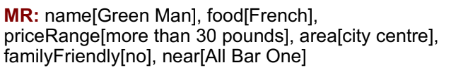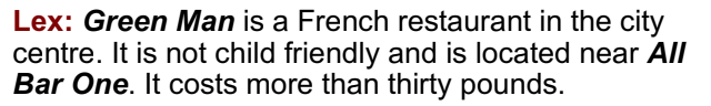Noise Injection and Self-Training

Aim: use data augmentation to create diverse MR/utterance pairs not seen in the training distribution

the delexicalization technique would have created pairs of the same syntax/from same template

Basically we would need two constraints for this to work:

text of a MR being diverse but is still related to the task (Base Speaker)
the correct MR corresponding to the above text (MR Parser)

Without Noise	With Noise = Data Augmentation

Hence we have a synthetic text and MR pair, but the pair is still faithful! The overall algorithm looks like

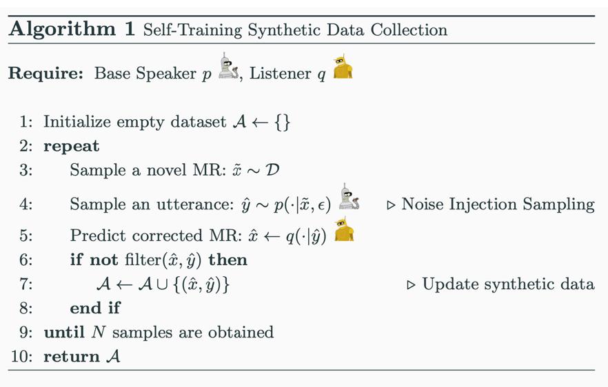
where

to make sure the new pair is not too bad/unclean, we also added a filter.
in the end you return $A$ which is the augmented dataset.

Train new seq2seq model on training + synthetic data: $D \cup A$. The new trained model is the called the Faithful Speaker

For example:

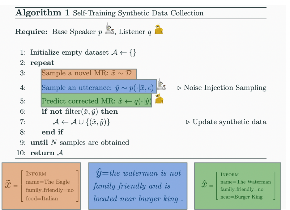
The advantage of this v.s. the delexicalization is that the generated text would have:

variety in words used (which delexicalization also can do)
variety in sentence structure (which delexicalization cannot)

E2E Metrics and Baseline

Some common metrics used include

Precision: want fulfilled tokens being correct
Recall: want to have fulfilled most of the tokens.
Semantic Error Rate (SER):
\[\frac{\text{\# missing}+\text{\# incorrect}+\text{\# added}}{\text{\# attributes}}\]
basically the denominator is the sum of cases where the attributed was not fulfilled.

Baselines used in this task

SLUG: ensemble of seq2seq models (e.g. transformer based, LSTM based, etc)
- pooled overgeneration+reranking
DANGNT (Nguyen and Tran, 2018): rule-based model
- basically from the corpus, extract statistically
TUDA (Puzikov and Gurevych, 2018): template-based model

With their performance being

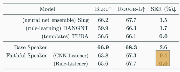
where we see Faithful speakers are performing better.

Next Word Sampling

Next Word Sampling means deciding how to pick the next word $w_t$ according to its conditional probability distribution $P(w_t\vert w_{1:t-1})$

Here we will see:

Greedy Search: what we do most of the time, so that at each time $t$ of decoding, we pick the single most probable words. However, the problem is that this might not generate the most probable sequence
Beam Search: Beam search reduces the risk of missing hidden high probability word sequences by keeping the most likely num_beams of hypotheses at each time step and eventually choosing the hypothesis that has the overall highest probability. But still, it does not solve the problem.
Top-k Sampling: it is a sampling method (i.e. randomly choose) from the Top-$k$ most likely next word based on redistributing the probability mass only among those $k$ words
Temperature Sampling: essentially rescaling the probability by temperature $T$, such that with $T$ is low only high energy (probability) would be “survive”, and when $T$ is high, low energy states gets a greater chance than before to be sampled.

Recap:

Beam Search: recall that the basic idea under beam search is that it keeps the $k$ most probable at each time step

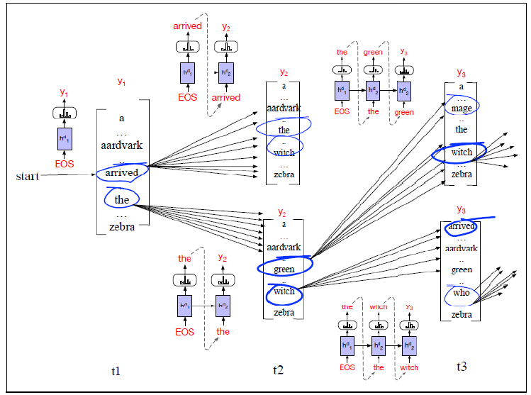
which can be done by:

have $k$ decoders ready
at each time step:
- keep $k$ most probable choice
- generate the next word from the $k$ most probable using the decoders
- prune down to the $k$ most probable and repeat

Top-k Sampling

Top-k Sampling: at each time step we get $P(w_t\vert w_{1:t-1})$ from our model:

sample from the Top-$k$ most likely next word based on redistributing the probability mass only among those $k$ words
this is used in GPT-2

This works because notice that at $t=2$, the top-k choices would have included most of the probability distribution already:

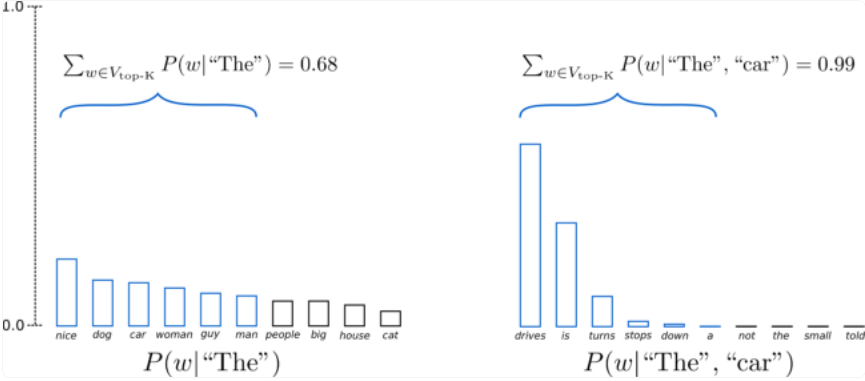
Temperature Sampling

Temperature sampling works by increasing the probability of the most likely words before sampling. The idea is borrowed from thermodynamics where essentially energy $\approx$ probability so that:

high temperature means low energy (probability) states are more likely (than the were before) to be encountered

lowering the temperature allows you to focus on higher energy (probability) state

So that given a probability distribution $P(x)$:

scaled probability by temperature $T$ is $z_i = \log P(x_i)/T$
then get back probability using softmax $\exp(z_i)/\sum \exp(z_i)$

For instance, we can take $T=2$ being a low temperature:

$P(x)$	$z_i$	Temperature Rescaled

where we see that with low temperature, only high probability terms “survives”. Result-wise:

high temperature sample displays greater linguistic variety
low temperature sample is more grammatically correct

Text Summarization

The high level task of summarization would include:

input: a database, an image, texts, software traces, etc
output: a textual summary

Essentially those types of generation models can all be seen as next word generation, but conditioned on different things:

pure next word generation:
\[p(y_{i+1}|y_{i-L+1:i})\]
for a window size of $L$ (depending on your machine’s memory for NN models) and $y_{i-L+1:i}$ are the words generated so far. Note that this is basically language models
\[p(w_{i+1}|w_{i-L+1:i})\]
which we have learnt in the beginning of NLP.

next word generation conditioned/based on some input sentence $\vec{x}=x_1,…,x_n$ as well:
\[p(y_{i+1}|\vec{x},y_{i-L+1:i})\]
which you will see is what summarization/conditional generation is essentially about: modelling the above probability with some neural network.

Currently this field does not have the best performances. Why is this task hard?

require both interpretation and generation of text
handle input documents from unrestricted domains robustly (e.g. trained on one domain but genearlize to news, military, entertainment)

Types of Summarization

In general, we can have the following types of summarization tasks:

informative v.s. indicative: generated content can replacing the document v.s. just describes the document
extractive v.s. abstractive: pick best $k$ words that most important v.s. generate $k$ words
single v.s. multi-document: many coming form different domains
generic v.s. user-focused: decides if we should use layman terms (e.g. commonly when in medical/legal domain, use professional terms)

Here, we will focus on mainly doing informative summarization and compare:

simple task of extractive summary
using a NN model for abstractive summary

Extractive Summarization

The formal definition of the task would be as follows.

given: a fixed vocabulary $V$
input: a sequence of $M$ words with $x_1,…,x_M$
output: a sequence of $N < M$ words (e.g. known before generation) $x_{m_i} \in {x_1,…,x_M}$ such that
\[\arg\max_{m \in \{1,...,M\}^N}s(\vec{x},\vec{x}_{m})\]
is largest for $\vec{x}=x_1,…,x_M$ and $\vec{x}m=x{m_1},x_{m_2},…,x_{m_N}$, and $s$ is a scoring function yuo can generally customize. The most common one you will see for LM are:
\[s(\vec{x},\vec{x}_m) = \log p(\vec{x}_m | \vec{x})\]

The common solution for this is to treat it as a classification task:

for input word $x_i$, should it be included in output list
repeat, and output by concatenating those words

In fact, for humans summary writes, they often do cut and paste

81% of the sentences were constructed by cutting and pasting

Abstractive Summarization

Not only pick $k$ words/phrase, but also generate words/phrase that summarizes the content.

if we just concatenate sentences as above, they might not be coherent

Formally, such a task can be defined as

given: a fixed vocabulary $V$
input: a sequence of $M$ words with $x_1,…,x_M$
output: a sequence of $N < M$ words (e.g. known before generation) $y_1,…,y_N$ such that
\[\arg\max_{\vec{y}\in \mathcal{Y}}s(\vec{x},\vec{y})\]
basically for $y_i \in V$, and $s$ is a scoring function you can generally customize. The most common one you will see for LM are:
\[s(\vec{x},\vec{y}) = \log p(\vec{y} | \vec{x})= \sum_{i=0}^{N-1} \log p(y_{i+1}|\vec{x},y_{1:i})\]
which is again(conditional) next word generation, and is often solved greedily using auto-regressive decoder.

You will soon seen in the Attention Based Summarizer how this probability $\log p(\vec{y} \vert \vec{x})$ can be modelled using a neural network.

Attention Based Summarizer

Here we discuss essentially a model proposed here: https://arxiv.org/abs/1509.00685, which is used for headline generation:

Input:	A detained iranian-american academic accused of acting out against national security has been released from a tehran prison yesterday after a hefty bail was posted, a top judiciary official said Tuesday.
Output:	Detained iranian-american academic released from prison after hefty bail.

Recall that we essentially need to model:

\[s(\vec{x},\vec{y}) = \log p(\vec{y} | \vec{x})\]

Since you will be using attention based model, the hidden representation for output will be applied over some attention layer. First, just like how we derived unigram/bigram/etc models:

\[p_\theta(\vec{y}|\vec{x})=p_\theta(y_1,...,y_N|x_1,...,x_N) = \prod_{i=1}^{N-1}p_\theta(y_{i+1}|\vec{x},y_{1:i})\]

being exactly true, but since for attention based model we need some predefined sequence length $C$ (as opposed to RNN type where you can encode a variable length by just looping it) such that:

\[\prod_{i=1}^{N-1}p_\theta(y_{i+1}|\vec{x},y_{1:i}) \approx \prod_{i=1}^{N-1}p_\theta(y_{i+1}|\vec{x},y_{i-C+1:i})\]

and hence for $s(\vec{x},\vec{y}) = \log p(\vec{y} \vert \vec{x})$ we get:

\[\log p(\vec{y}|\vec{x}) \approx \sum_{i=0}^{N-1} \log p_\theta(y_{i+1}|\vec{x},y_{i-C+1:i})\equiv \sum_{i=0}^{N-1} \log p_\theta(y_{i+1}|\vec{x},\vec{y}_C)\]

being our model.

Then for NN based model, essentially the idea is to do:
\[p_\theta(y_{i+1}|\vec{x},\vec{y}_C) = \text{Softmax}(W \, \text{repr}(\vec{x},\vec{y}_C)) \in \mathbb{R}^{|V|}\]
so that $W \in \mathbb{R}^{\vert V\vert \times H}$ for $\text{repr}(\vec{x},\vec{y}_C)$ being some vector of hidden dimension $H$.

For this paper, we consider:

\[p_\theta(y_{i+1}|\vec{x},\vec{y}_C) = \text{Softmax}(V\vec{h} + W\,\text{enc}(\vec{x},\vec{y}_C)) \in \mathbb{R}^{|V|}\]

for the first part being empirically useful to have as:

$\tilde{y}C = [Ey{i-C+1},…,Ey_{i}]$ are the embedded generated outputs
$h = \tanh(U \tilde{y}_C )$ producing a single vector summarizing what we have so far

So basically we have the general architecture of splitting this to an encoder-decoder architecture:

encoder: do the $\text{enc}(\vec{x},\vec{y}_C)$ part and get a vector of hidden dimension $H$
decoder: do the $\text{Softmax}(V\vec{h} + W\,\text{enc}(\vec{x},\vec{y}_C))$ part with auto-regressive generation

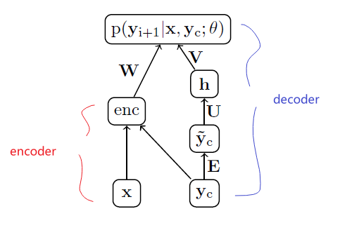
where:

for attention based summarizer, the encoder part is essentially an attention based encoder
however, of course you can customize what you do at that encoder

Baseline BoW Encoder

Consider the simple framework of doing:

Encode all the input but ignoring generated context:
\[\tilde{x} = [Fx_{1},...,Fx_{M}]\]
for $F \in \mathbb{R}^{H \times \vert V\vert }$
Then we consider a uniform distribution
\[\vec{p} = [1/M,...,1/M]\]
so that
\[\text{enc}_1(\vec{x},\vec{y}_c) = \vec{p}^T \tilde{x}\]

so then the entire encoder network only needs $\theta_{enc} = {F}$

Convolutional Encoder

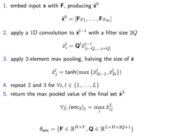
Attention Based Encoder

Algorithm	Architecture

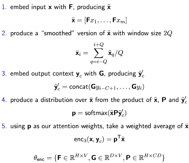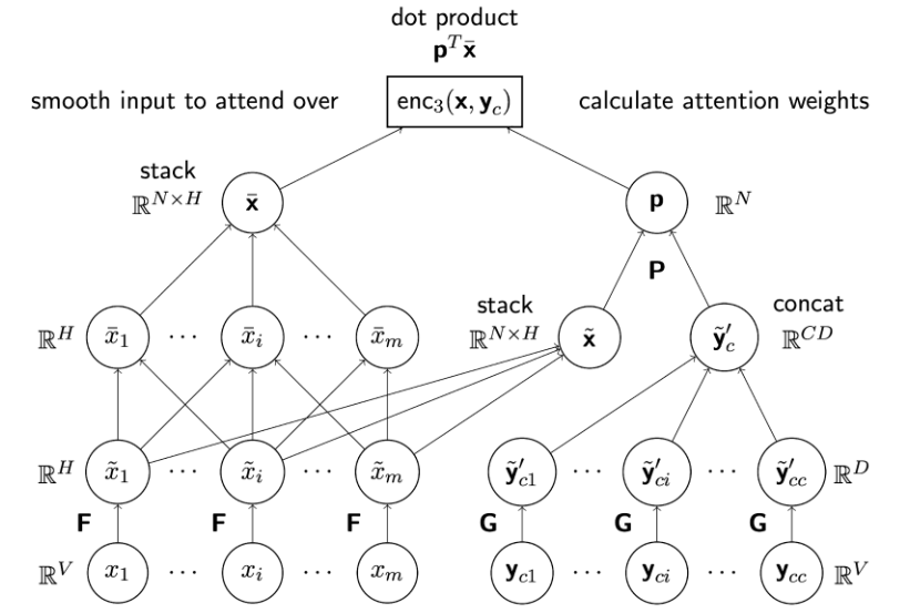which performs better than the others:

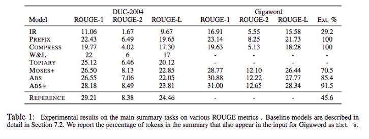
BART

Now, essentially for text generation we want some architecture that does:

encoder: encode input $\vec{x}$
decoder: uses $\text{enc}(\vec{x})$ and some representation of $\vec{y}_C$ to generate:

Hence we can use a classical architecture:

Idea	BART Pretrain

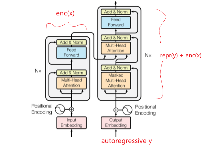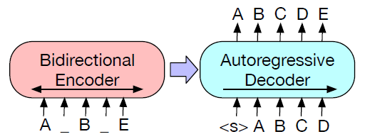which essentially does:

\[p_\theta(y_{i+1}|\vec{x},\vec{y}_C) = \text{Softmax}( \text{repr}(\vec{x},\vec{y}_C)) \in \mathbb{R}^{|V|}\]

where here $\text{repr}(\vec{x},\vec{y}_C)$ would come from weigths that does:

embedding of $\vec{x}, \vec{y}c$ using two networks $f\theta(\vec{x}),g_\phi(\vec{y})$
- in contrast to generation with GPT, which only has a single network for encoding $f_\theta(\vec{x}), f_\theta(\vec{y})$
doing multi-head attentions
doing FFNN and others.

But essentially we comes down to having some good encoding network. Therefore BART consider pre-train tasks of corrupting documents and then optimizing a reconstruction loss:

and notice that In the extreme case, where all information about the source is lost, BART is equivalent to a language model.

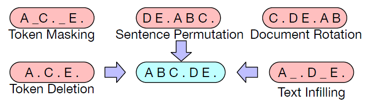
Then, once trained, we fine-tune on a range of tasks

Sequence Classification: the same input is fed into the encoder and decoder, and the final hidden state of the final decoder token is fed into new multi-class linear classifier.
- basically related to the CLS token in BERT
(Conditional) Sequence Generation: the encoder input is the input sequence (to be conditioned on), and the decoder generates outputs autoregressively

Comparison Against GPT and BERT

What is special about using both encoder-decoder for the task of generation? Recall that:

BERT	GPT	BART

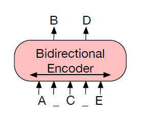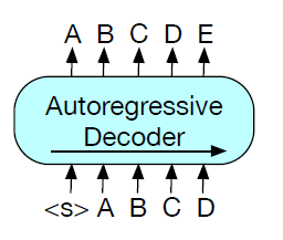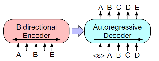so that:

BERT: Random tokens are replaced with masks, and the document is encoded bidirectionally. Missing tokens are predicted independently, so BERT cannot easily be used for generation
GPT: Tokens are predicted auto-regressively, meaning GPT can be used for generation. However words can only condition on leftward context, so it cannot learn bidirectional interactions.
- also it uses the same encoding network at all times
BART: Inputs to the encoder need not be aligned with decoder outputs, allowing arbitrary noise transformations, i.e. can generate “new words” for tasks such as summarization.
- then the likelihood of the original document (right) is calculated with an autoregressive decoder
- notice that the order changed as this is allowed for encoder-decoder type model! We are using two networks $f_\theta(\vec{x}),g_\phi(\vec{y})$ for encoding the input and the output generated differently, as their interaction could be complex

Chatbots & Dialogue Systems

This chapter introduces the fundamental algorithms of dialogue systems, or conversational agents. These programs communicate with users in natural language (text, speech, or both), and fall into two classes:

Task-oriented dialogue agents use conversation with users to help complete tasks. Examples include Siri, Alexa, Google Now/Home, Cortana, etc., which can give directions, control appliances, find restaurants, or make calls.
- for those products, we also needed Automatic Speech Recognition and Text to Speech with an architetcure
  
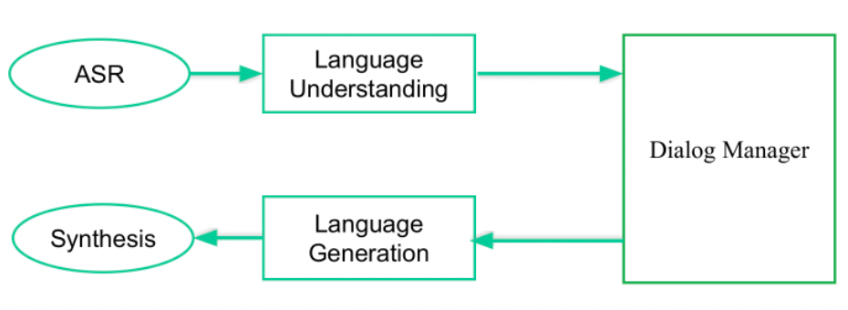
  where basically dialogue manager decides what actions to take
chatbots are systems designed for extended conversations, set up to mimic the unstructured conversations or ‘chats’ characteristic of human-human interaction
- mainly for entertainment
- but also for practical purposes like making task-oriented agents more natural.

we’ll discuss the :

three major chatbot architectures: rule-based systems, information retrieval systems, and encoder-decoder generators.
for task-oriented agents, we introduce the frame-based architecture (the GUS architecture) that underlies most task-based systems

Properties of Human Conversation

Before we attempt to design a conversational agent to converse with humans, it is crucial to understand something about how humans converse with each other. For example:

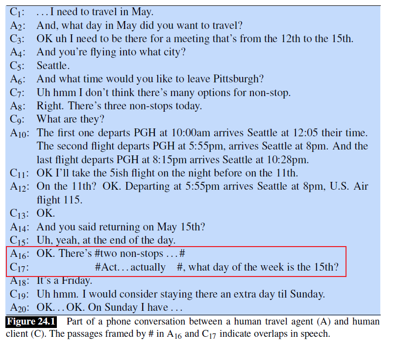
where C stands for client and A stands for Agent

A dialogue is a sequence of turns (C1, A2, C3, and so on)
- A system has to know when to stop talking; the client interrupts (in A16 and C17), so the system must know to stop talking
- A system also has to know when to start talking. e.g. Spoken dialogue systems must also detect whether a user is done speaking, so they can process the utterance and respond.
  
  This task is called endpointing or endpoint detection
Speech/Dialog Acts: each utterance in a dialogue is a kind of action being performed by the speaker. Basically expresses an important component of the intention of the speaker (or writer) in saying what they said
Grounding: acknowledging that the hearer has understood the speaker (e.g. saying “OK”, as the agent does in A8 or A10.)
Sub-dialogues and Dialogue Structure: QUESTIONS and ANSQWE, PROPOSALS and ACCEPTANCE/REJECTION, etc. These pairs, called adjacency pairs are composed of a first pair part and a second pair part
- However, dialogue acts aren’t always followed immediately by their second pair side sequence part. The two parts can be separated by a side sequence
- e.g. utterances C17 to A20 constitute a correction subdialogue; another common one would be clarification questions
Initiative: whoever is taking the lead in the conversation is taking initiative. In normal human-human dialogue, however, it’s more common for initiative to shift back and forth between the participants
- Mixed initiative, when initiative shifts between the two people, is very difficult for dialogue systems to achieve.
- In contrast, the QA system would be a user-initiative system: user specifies a query, and the systems passively responds.
- It’s much easier to design dialogue systems to be passive responders.
Inference and Implicature: consider

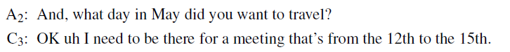
Notice that the client does not in fact explicitly answer the agent’s question. We need to inference the answer.

Chatbots

The simplest kinds of dialogue systems are chatbots systems that can carry on extended conversations with the goal of mimicking the unstructured conversations or characteristic of informal human-human interaction

A recent example would be Facebook’s BlenderBot:

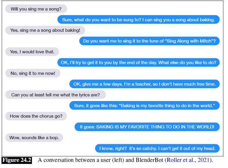
Like practically everything else in language processing, chatbot architectures fall into two classes: rule-based systems and corpus-based systems

Rule-based systems include the early influential ELIZA and PARRY systems
Corpus-based systems are more modern:
1. mine large datasets of human-human conversations,
2. generate responses by either
  - using information retrieval to copy a human response from a previous conversation
  - using an encoder-decoder system to generate a response from a user utterance

Corpus-based Chatbots

Corpus-based chatbots, instead of using hand-built rules, mine conversations of human-human conversations. These systems are enormously data-intensive, requiring hundreds of millions or even billions of words for training.

Most corpus based chatbots produce their responses to a user’s turn in context either by

retrieval methods: using information retrieval to grab a response from some corpus that is appropriate given the dialogue context
generation methods: using a language model or encoder-decoder to generate the response given the dialogue context

Essentially the two architectures look like:

Retrieval Based	Generation Based

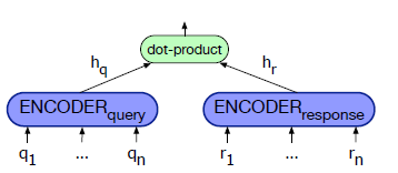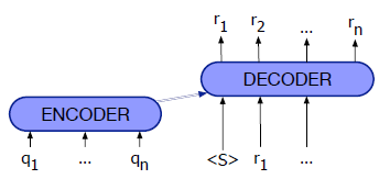So that given a training corpus $C$ which contains many conversations, and given a user’s query being $q$, we consider:

Retrieval based: return some appropriate turn $r$ as response by:

\[r = \arg\max_{r \in C} \frac{q \cdot r}{|q||r|}\]

where $q,r$ could be vectors computed by:

TF-IDF encoding
train an encoder for query and one for response (left figure in the above)

For instance, we could train two encoders by fine-tuning BERT so that we get $\text{BERT}_Q,\text{BERT}_R$:

\[h_q = \text{BERT}_Q(q)[CLS]\\ h_r = \text{BERT}_R(r)[CLS]\]

where recall that the CLS token is used to encode the entire sentence. Then:

\[r = \arg\max_{r \in C} h_q \cdot h_r\]

Generation Based: think of response production as an encoder-decoder task — transducing from the user’s prior turn to the system’s turn. So basically can treat it as a kind of translation.

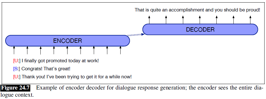
Recall that for encoder-decoder models, it is auto-regressively generating but conditioned on the entire query $q$:

\[\hat{r}_{t+1} = \arg\max_{w \ni V} P(w|q,r_1,...,r_{t})\]

but sometimes instead of just user’s query, we can encode the entire conversation to be conditioned on.

Other ideas for generation:

fine-tune a large language model/decoder only on a conversational dataset and use the language model directly as a response generator.
https://arxiv.org/pdf/1606.01541.pdf using Deep Reinforcement Learning
https://aclanthology.org/D17-1230.pdf using Adversarial Learning

GUS: Simple Frame-based Dialogue Systems

We turn now to task-based dialogue, in which a dialogue system has the goal of helping a user solve some task like making an airplane reservation

First some terminologies:

A frame is a kind of knowledge structure representing the kinds of intentions the system can extract from user
A frame consists of a collection of slots, each of which can take a set of possible values.
- basically specifies what the system needs to know
A set of frames is sometimes called a domain ontology.

For example, in the travel domain:

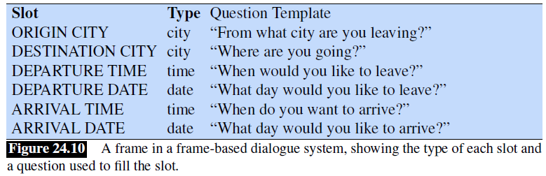
where:

a lot might be of type city, date, time
this would be an example of a frame
technically, many Types in such a system is itself a frame. For instance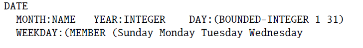

Control structure for frame-based dialogue

The system’s goal is to fill the slots in the frame with the fillers the user intends, and then perform the relevant action for the user (answering a question, or booking a flight).

To do this, the system need to do:

asks questions of the user (using pre-specified question templates associated with each slot of each frame)
- If a user’s response fills multiple slots, the system fills all the relevant slots, and then continues asking questions to fill the remaining slots
- there are also condition-action rules attached to slots. For example: a rule attached to the DESTINATION slot for the plane booking frame, once the user has specified the destination, might automatically enter that city as the default StayLocation for the related hotel booking frame.
Many domains require multiple frames. Then this control system needs to disambiguate which slot of which frame a given input is supposed to fill
Once the system has enough information it performs the necessary action (like querying a database of flights) and returns the result to the user

Exactly how do we do step 1 and 2? This is in the section covered below.

Determining Domain, Intent, and Slot fillers in GUS

How do we implement the above control system? We need to essentially do three things:

The first task is domain classification: is this user for example talking about airlines?
user intent determination: what general task or goal is the user trying to accomplish?
Finally, we need to do slot filling: extract the particular slots and fillers that the user intends the system to understand

The slot-filling method used in the original GUS system, and still quite common in industrial applications, is to use handwritten rules

Generation in GUS

Finally, once all information are collected and necessary actions are performed by the system, we perform language generation to respond to user.

Frame-based systems tend to use template-based generation
or encoder-decoder network with dependency on the dialogue state (i.e. the question user just asked)

The Dialogue-State Architecture

Modern research systems for task-based dialogue are based on a more sophisticated version of the frame-based architecture called the dialogue-state or or belief-state architecture.

Moderm architecture looks like the following:

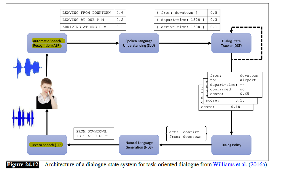
where:

for audio input/output, we had this extra two modules on the left
the other four components are part of both spoken and textual dialogue systems
- For example, like the GUS systems, the dialogue-state architecture has a component (Natural Language Understanding Module) for extracting slot fillers from the user’s utterance, but generally using machine learning rather than rules.
- The dialogue state tracker maintains the current state of the dialogue (which include the user’s most recent dialogue act, plus the entire set of slot-filler constraints the user has expressed so far).
- dialogue policy decides what the system should do or say next: e.g. wen to ask clarification question, when to make a suggestion, etc.
- natural language generation: condition on the exact context to produce turns that seem much more natural

Dialogue Acts

Different types of dialogue systems require labeling different kinds of acts, and so the tagset—defining what a dialogue act is exactly— tends to be designed for particular tasks. For example

Dialogue Act	Labelled Conversation

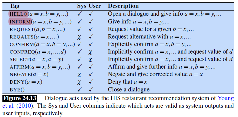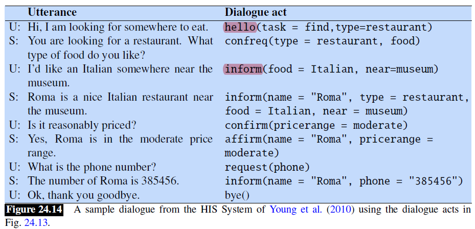note that the above example also showed the content of each dialogue acts, which are the slot fillers being communicated

Slot Filling

Here, we discuss how the task of slot-filling, and the simpler tasks of domain and intent classification, are typically done. This is still part of the job of the Natural Language Understanding Module.

We consider the following situation:

input: “I want to fly to San Francisco on Monday afternoon please”
output: domain is AIRLINE, intent is SHOWFLIGHT, and the fillers being

A simple architecture that does is is simply:

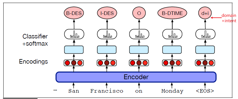
which is basically a Sequence classification model such that:

we use BERT to embed each input
then pass though FFNN with a softmax so that:
- for each word, decide which tag it is
- for the last tag <EOS>, use SoftMax to classify which intent and domain it is

Then, once the sequence labeler has tagged the user utterance, a filler string can be extracted for each slot from the tags (e.g., “San Francisco”), and these word strings can then be normalized to the correct form in the ontology

Dialogue State Tracking

The job of the dialogue-state tracker is to determine both the current state of the frame (the fillers of each slot), as well as the most recent dialogue act.

Since dialogue acts place some constraints on the slots and values, the tasks of dialogue-act detection and slot-filling are often performed jointly.

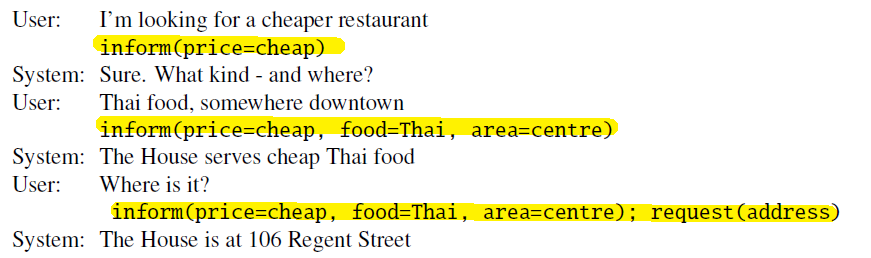
The simplest dialogue state tracker might just take the output of a slot-filling sequence-model. But more complicated cases include:

detecting correction acts
value being changed in the current sentence or should be carried over from previous sentences

Essentially it would be a condensed information that related to the entire conversation so far. This will be used in the next module to decide what policy to take.

Dialogue Policy

The goal of the dialogue policy is to decide what action the system should take next, that is, what dialogue act to generate.

Formally, at turn $i+1$ we want to predict what action $a_{i+1}$ to take, which would be based on the entire sequence of dialogue:

\[\hat{a}_{i+1} = \arg\max_{a_{i+1} \in A}P(a_{i+1}|s_i)\]

for $s_i$ the state being encoded with representation of:

current state of Frame $i$
previous user and system dialogue actions
etc.

Learning a best policy would be done by reinforcement learning system gets a reward at the end of the dialogue, and uses that reward to train a policy to take actions.

Additionally, this module might need to take on task of choosing some attributes (slots and values) which plans on what to say to the user, before feeding into the NLG module.

Natural Language Generation Module

Once a dialogue act has been decided, we need to generate the text of the response to the user.

The task of natural language generation (NLG) in the information-state content architecture is often modeled in two stages:

content planning (what to say)

sentence sentence realization (how to say it).

Here we assume that the previous module has chosen the dialogue act to generate, and chosen some attributes (slots and values) that the planner wants to say to the user.

Example input/output looks like

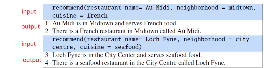
where In the first example:

the content planner has chosen the dialogue act RECOMMEND and some particular slots (name, neighborhood, cuisine) and their fillers
The goal of the sentence realizer is to generate a sentence like lines 1 or 2 shown in the figure (here we have two samples as we can sample the generation module again and get a different output)

However, the problem here is training data: it is hard ot get a good combination of every possible act/slots:

Therefore it is common in sentence realization to increase the generality of the training examples by delexicalization (basically remove the formal nouns, so we get a template)
or any other data augmentation tricks such as Noise Injection and Self-Training

Persuasive System

This is a more advanced system, which is technically a task-oriented system but with the aim of persuading people to do something, So, to achieve that goal, certainly some social aspects of the conversation is needed.

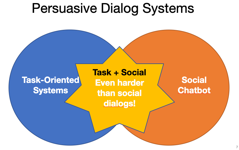
Some potential uses of this system include:

exercise persuation
suisicde counseling (train counseller by acting as a visitor)
social distancing

Again, the aim is to change people’s belief and behavior (might have ethnical issues). How do we do that using machine learning?

Challenges in Persuasion

The basics of data-driven methods for persuasion includes the following three modules:

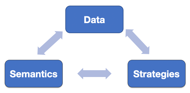
where:

like all tasks, it is important to collect some good data
then, we want our chatbot to be able to understand the semantics of user’s utterance (i.e. what they said)
finally, it moves on to persuade by picking some strategy (and then generate text response)

Data Challenges

To start a good project/model, first we need to collect good data.

Like many ML tasks, collecting good data is always important. But that is not easy because even chaning a single word in a sentence could have lead to an entire new utterance. Therefore, the set of conversation path with each node being a sentence is exponential

so ideally we want our training data to cover all possible dialog trajectories, but that is intractable. Hence some approaches include

learning a subset of the tree and hope for the best
try to merge different branches to make the tree smaller
etc.

Additionally, as our aim is an optimization task, there could be different optimal path for a different user to be persuaded

so that given some user information/background, the system needs to pick an optimal path down the tree for that particular user

Semantic Challenges

Many large models are able to make language generation fluent, but they often do not understand deep level semantics of the language (e.g. Microsoft’s Tay AI), which can lead to unsafe systems.

one potential task on this direction would be: how do we build a system that can “filter out” those dangerous generated languages?

Strategy Challenges

In certain scenario, some persuasive strategy would be more effective than another.

for instance, hearts and cakes could be more persuasive than pizzas in this scenario.

Dialog Data Collection

How do we get dialog data?

production dialog (i.e. companies with their customers) are not available due to privacy issues.
- a good source would be customer services, but again there are privacy issues
role-play persuasion would be ineffective if there is lack of incentives. So persuasive quality might not be good.

Then people decided to use monetary incentive (i.e. using CrowdFlower/Mechanical Turks), with the persuasion task of donation:

persuaders receive bonus when persuadees donate
persuadees donation sent to the charity
also collect big-five personality of the persuadee (for personalization system)

Hence the overall work flow looks like:

Some examples include: (Persuasion for Good dataset)

where the person on the left will be the crowd-funded persuader.

Hierarchical Intent Annotation

We also want to build a system that understand some semantics of the sentences/dialogs.

so not just fluency, but also semantics

The idea is to annotate each sentence an intent/dialog act, which can be hierarchical

where MIDAS were used for social chatbot annotation.

An example of annotated piece of dialog would be

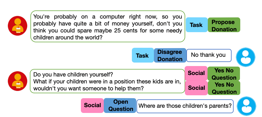
Classic Modular Dialog System

Recall that we had the framework for dialog system, usually it looks like

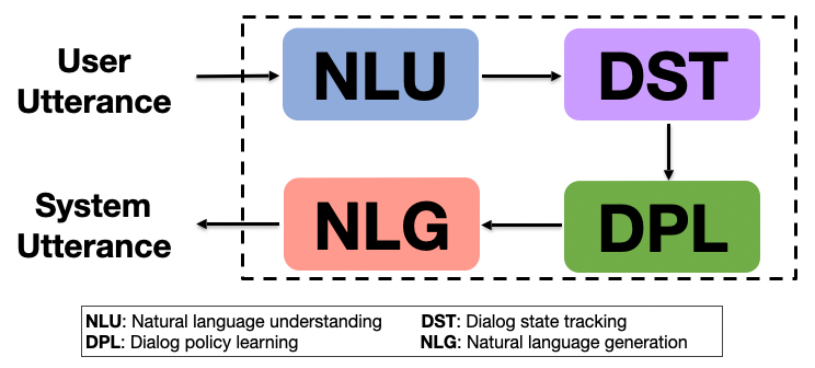
where in particular:

Module Name	Input/Output
NLU
DST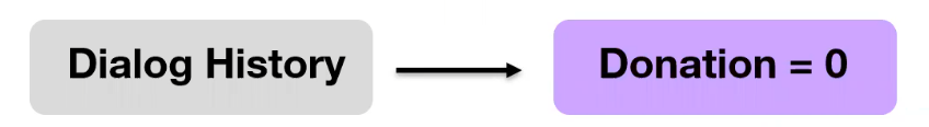
DPL
NLG

NLU: will be to understand the user’s utterances (i.e. semantic intent of the sentence)
- usually used for intent detection, then any Seq-classification model would work (as we have a limited intent)
- usually it is used per sentence based, which is why we needed some kind of accumulator later which is the DST
DST: input dialog history, output slot and values
- the aim is to track dialog state: sequence of information that is critical to remember
- e.g. for restaurant domain: how much food you want, location of restaurant
- e.g. for donation persuasion: how much donation we got for far, etc.
DPL: given the current state and user’s input, what policy/action should we take now?
- e.g. maybe we should provide some facts now
NLG: given the action we want to take, generate the output languages

Now with a modular network, we can train it:

each module separately
jointly/end-to-end
some other way

Modular Training Drawbacks

The problem with this kind of training is that:

heavy expert involvement, to tune each module
hard to tune individual modules, hence usualy need end-to-end trainng
heavy manual annotation needed for training data
- because each module needs different input/output

End-to-End Drawbacks

Avoiding the training/data annotation problem for modular training, we can train end-to-end:

which has been done on social chatbots a lot, such as GPT-2

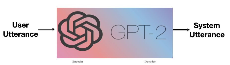
However, here we also have problems:

difficult for error analysis: you don’t know which module went wrong! (DST error? NLG error?)
since they don’t have semantic controls, we nede a large amount of data to train

MOSS: A combination

Here we combine the best of both types:

use one encoder (shared), but four decoders (separated)

The aim is to build a system that is end-to-end trainable but also trainable in a modular fashion (without going out of sync):

Architecture	Pipeline

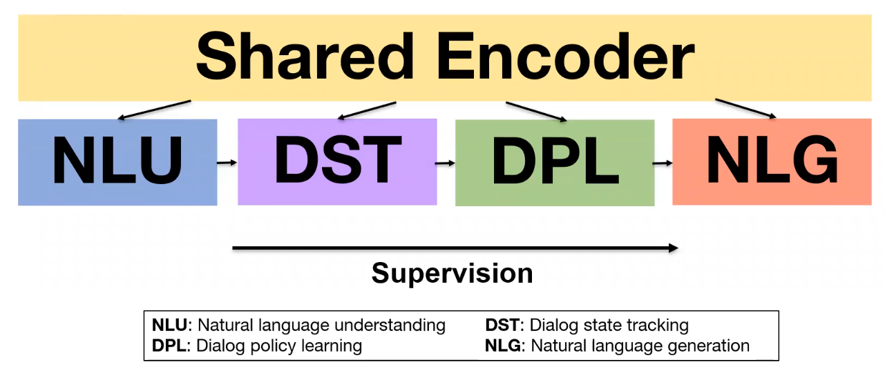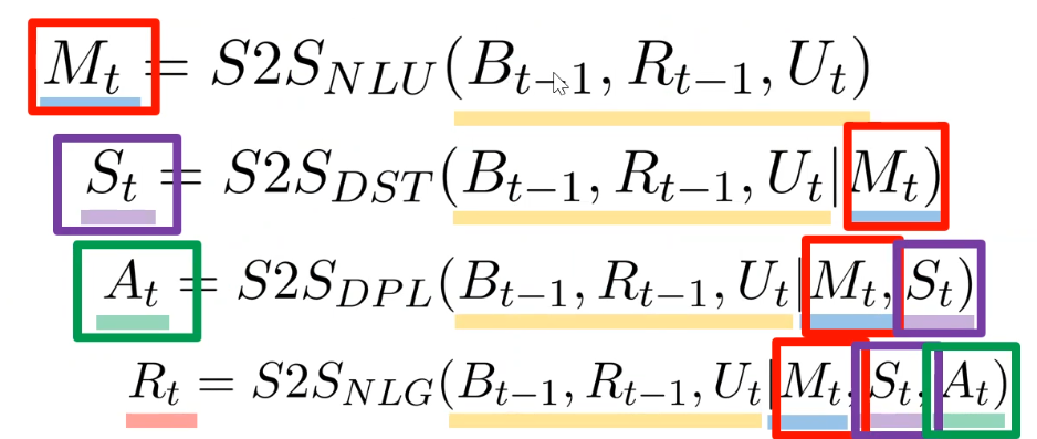where:

for end-to-end training, the shared encoder weights will only be updated once
for modular training, shared encoder will also be updated so its “knowledge” can still be used in other modules (in sync)
as you see in the pipeline, essentially each module uses output of the shared encoder but conditions/uses on the output of the previous module as well

One key advantage of this architecture is that we can train it even if we only have partial labels (e.g. only have 30% fully labelled, or only 40% labelled with intent)

For instance:

Fine-tuning on donation persuasion: we only have 300 labeled but 700 unlabeled data. We can

first do end-to-end training: train all 1000 unlabeled on NLG, which does not need intent labeling
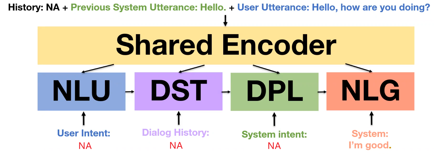
then do modular training: we can tune all again with 300 labelled to update the other three

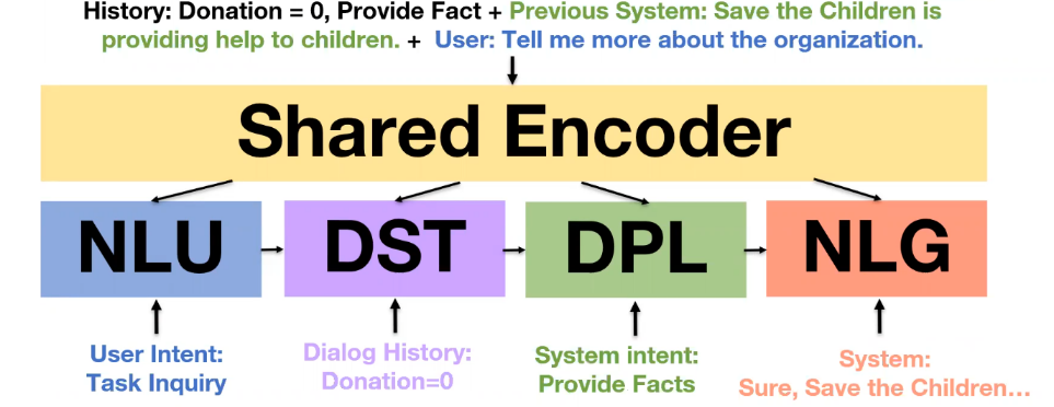
One take-away here is that it kind of depends how much data you have:

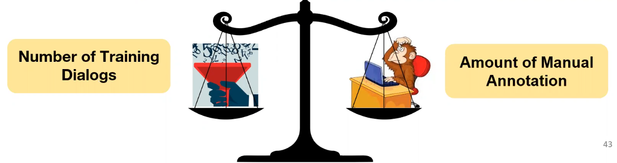
where:

if you have a lot of training dialogs then you might not even need to label them and it could work
if you don’t have much training dialogs, then having high quality labeled ones are needed

Other advantage of this kind of architecture is that:

easy to perform error analysis (we can decode the output for each module for a given input)
can handle complex task

Human Evaluation on Persuasion

To analyze the performance of the model simply:

compare against human persuaders: how many percent of persuadee did it succeed to persuade?
build a baseline: take GPT-2 and just tune end-to-end on all 1000 data

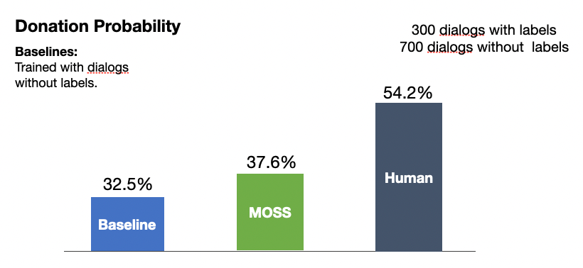
Why can human do so well? Where error analysis becomes important!

Error Analysis: Unfaithful Outputs

Checking on some outputs, we see that sometimes chatbot lies when It has never seen an utterance.

it failed to understand the semantics, and generated something related some the training data without understanding it

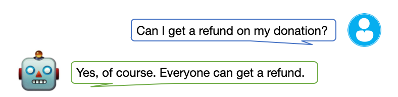
This can be dangerous in deployment. Therefore one approach is to have a safety net that can rank which responses is better

use beam search, nucleus sampling, temperature sampling, to get $N$ candidates
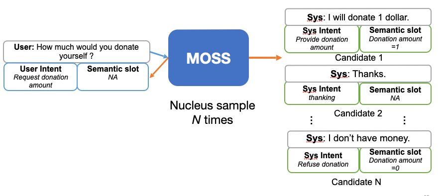
gather training data by having humans ranking it

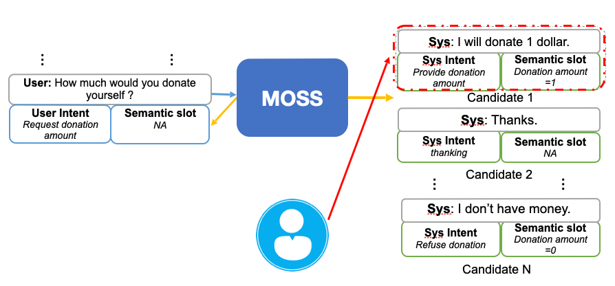
given some sampled $N$ samples, with the intent and semantic slot, rank those responses by a human in the loop
once we have samples of human ranking, train a classifier to rank it

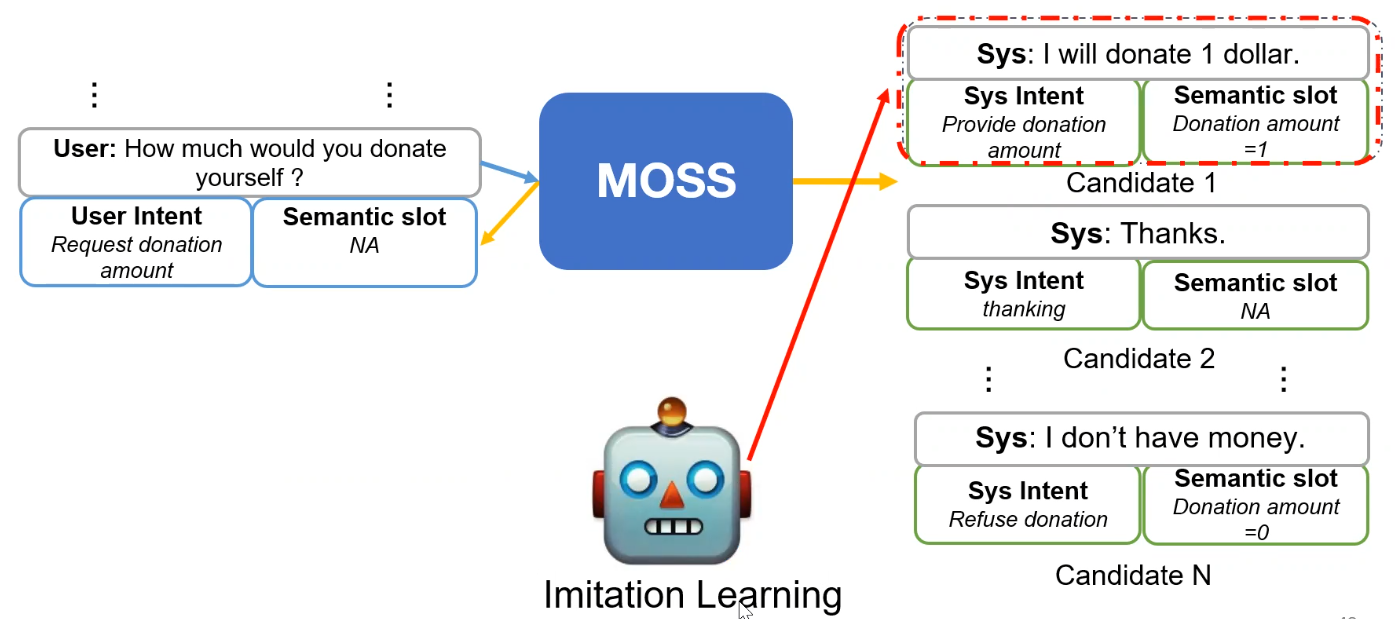
Then, after this fix, we got a 10% boost from the MOSS architecture

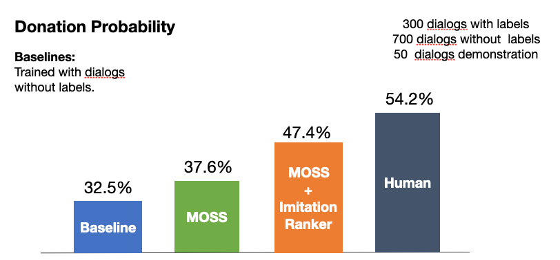
but still a bit less than human performance.

Error Analysis: Persuasion Strategies

Consider the following example

Failed Cases	Success Cases

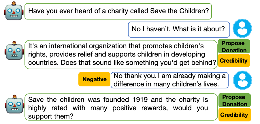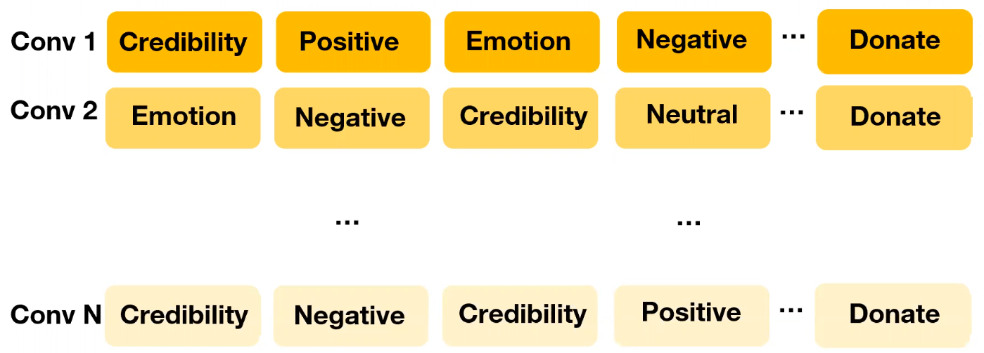where we see that there is a wide variety of actions to take than credibility appeals when persuading people.

Therefore, we also need persuasion strategies (i.e. how to persuade), in addition of the dialog act of propose-donation (by the DPL module, on what to do next)

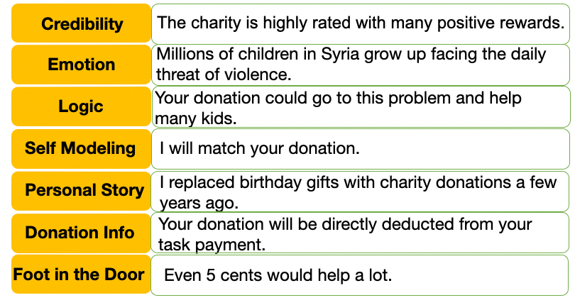
so we added this module of DSP: dialog strategy planning, into the pipeline

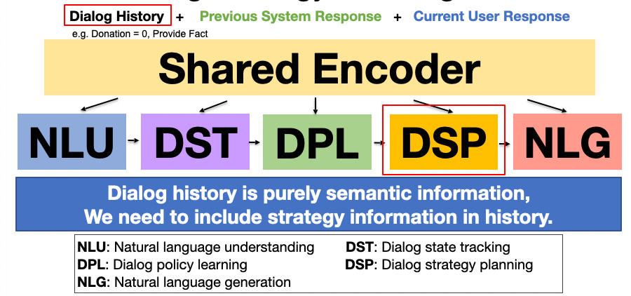
note that of course this module needs past trajectory of user’s intent/feedback as well as system’s intent to decide what is the best strategy to pick

Hence essentially this module will be learning the successful trajectories

e.g. a finite state transducer, or any RL type algorithm

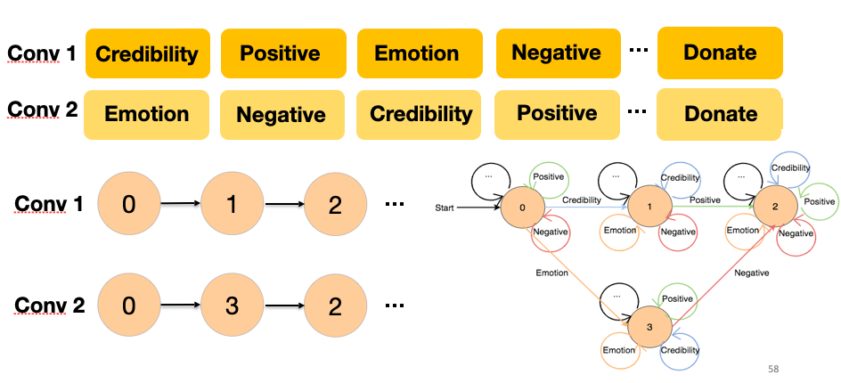
Finally, once added, this can further improve can be made

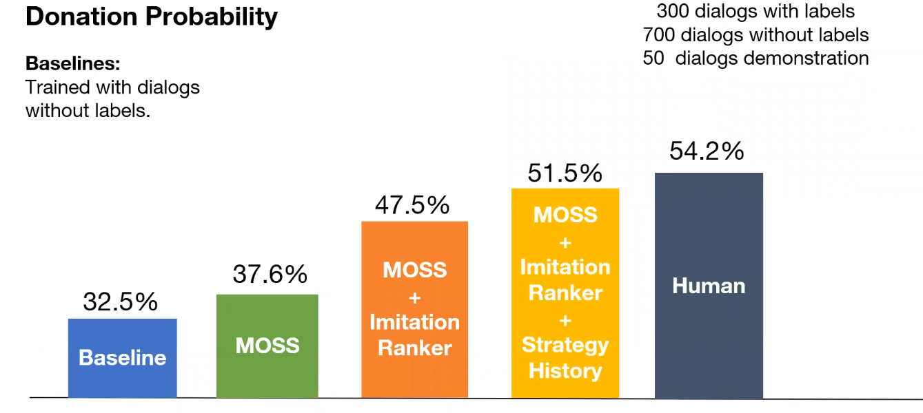
Error Analysis: Personality Adaptation

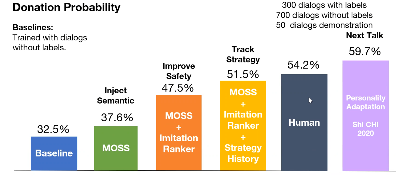
Dialogs is More than NLP

For production use in reality, dialogs requires much more than just NLP:

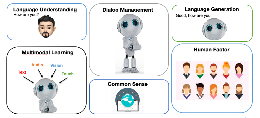
where the Language understanding, Dialog Management, and Language Generation would be handled by NLP. But we also need:

most of the time conversations are spoken: hence we have multi-modal data such as hand gestures and audio inputs
- e.g. speeches have much noise. Can we still recover the intent with noises?
- e.g. given some emotion of the speaker, what is the best strategy?
need common senses to deal with out-of-distribution conversations (e.g. erratic inputs)
other human factors used for judging the quality of conversations

Ethnical Consideration of Chatbots

36% of the people thought that they are humans (but they are mechanical turkers, so it depends on the education level)

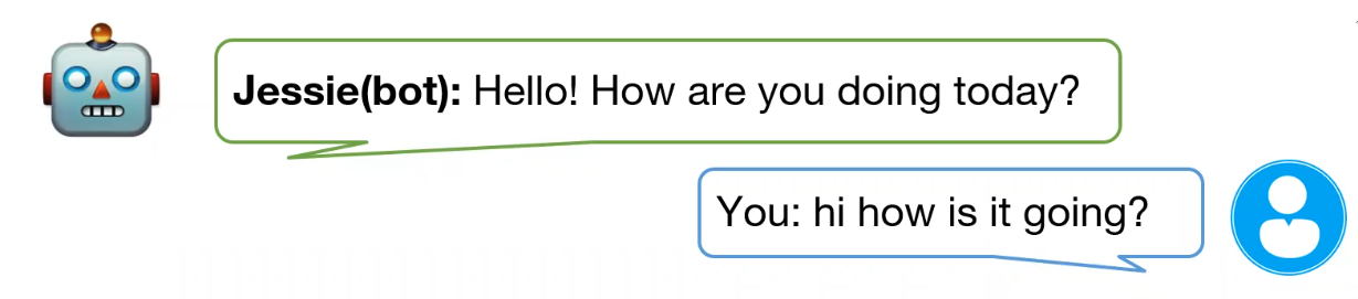
which can be very dangerous

e.g. scamming people for money.
but you could also train a bot to depend against scammers as well

But anyway

though it is rarely exercised.

Meta Learning in NLP

Useful when you have low resource (training sets), but you still want to achieve some task. Commonly, the familar methods you might know include:

taking a pre-trained model then fine-tune on your limited resource task (transfer learning)
but here, we will introduce a new method to solve this kind of problem

What is Meta-Learning

To understand what meta-learning is doing, we will see how we got from the transfer learning to the meta-learning task

transfer learning
multitask learning
meta-learning

Transfer Learning

Assume we have learnt a network and is trained for english to french translation with enough data.

But now we have a new task, which does not have enough data. But notice that we could had a simliar architecture

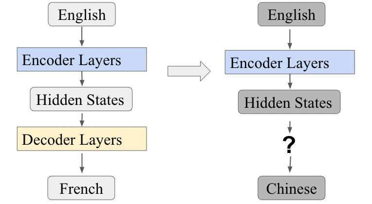
so that:

encoder layers should work in both cases because they are used to “understand english”
then, all we need to do is to fine-tune the decoder layers, which is essentially transfer learning.

This works pretty well because in reality, because good models typiocally have large encoder layers but only few decoder layers.

Multitask learning

Now suppose we are given a training dataset that have:

a lot of task (e.g. english to french, english to chinese, etc)
ach task has only a few training data

Data	Architecture

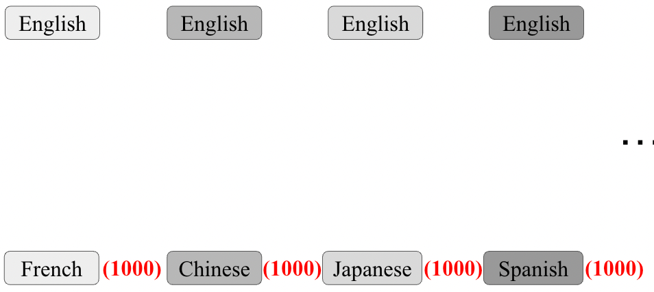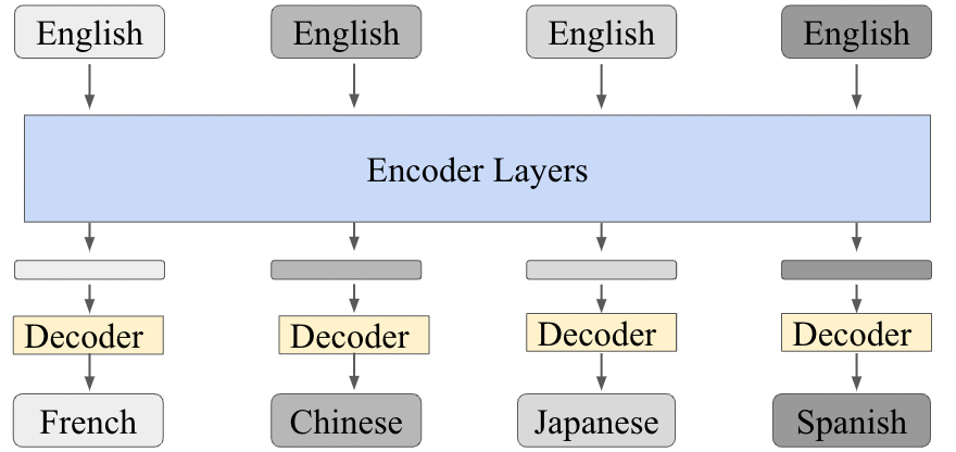the data for each language pair is too small, but it could be that all of them combined is enough. Then:

you have the architecture on the right, which has a shared encoder which learns through all training data
but what about the loss of that shared layer?
- the loss will most often be a linear combination of $L_i$ for task $T_i$
  \[\mathcal{L}(\theta^{sh}, \theta^1, ...,\theta^T) =\sum_{i=1}^T \alpha_i \mathcal{L}_i(\theta^{sh}, \theta^i, D_i)\]
  so that each task essentially is $\mathcal{L}_i(\theta^{sh}, \theta^i, D_i)$ for having a dataset $D_i$

Meta-Learning: two types of views of the task

Mechanistic View:
- normally we train by reading in the training dataset of samples, then inference on new sample
- here, we train with a dataset where each training sample is a dataset of a task $T_i$. This dataset will be called a meta-dataset
- of course, the aim of this is to perform well on a new task $T$ with its dataset
Probabilistic View:
- from the meta-dataset, we aim to extract a good prior that should be shared from those set of tasks
- then, doing a few-shot learning on a new task will use this prior and then train to infer posterior parameters

In general, on common application of this is to make it perform well under few-shot conditions.

Typical View	Meta-Learning

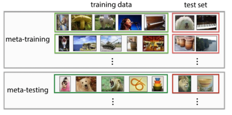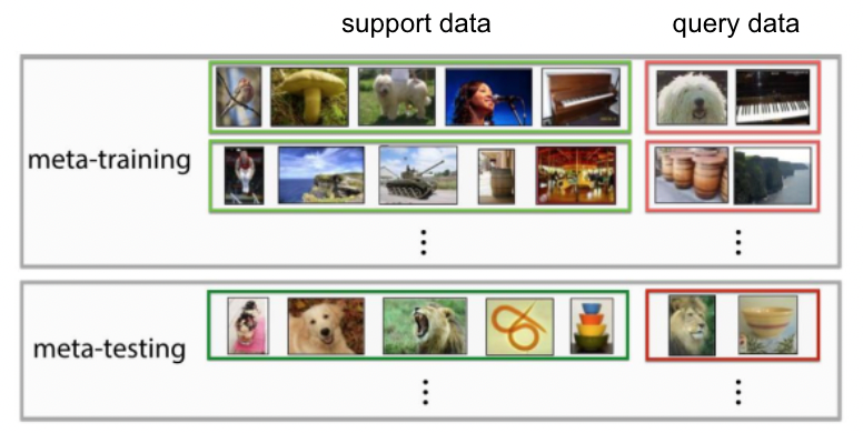so essentially we have:

at training: train support, train query sets
at testing: test support, test query sets
we want the model to perform well in test support and test query

Therefore, we want to simulate the testing environment during our training procedure

just like normal model training where our train/test environment are both classification, here our train/test environment should both be few-shot learning
how do we do this? Essentially see Model Agnostic Meta Learning

Meta-Learning Algorithms

Broadly speaking, there are two types of meta-learning algorithms:

Optimization Based: we still optimize over some loss of a model, but we introduce a new training paradigm that is suitable for donig few-shot learning at test time
- i.e. at test time, we can fine-tune our model fast when only given a few-shot training samples
Metric Based: learning a model that gives a good representation/embedding for each class $c_i$ (under few-shots), from which we can apply some metrics (e.g. distance) to measure, for a query sample $x_q$ which class $c_i$ is belongs to
- i.e. at test time, we directly use this model (which learns some metrics) when only given a few-shot training samples

Model Agnostic Meta Learning

Suppose we have some model $f_\theta$ we want to use, for example a CNN.

The goal of few-shot meta-learning is to train a model $f_\theta$ that can quickly adapt to a new task using only a few datapoints and training update iterations to $\theta$.

in other words, we want some good initialization of $\theta_0$ (learnt from other tasks as a “warm start”) such that in a new task it learns fast with only few samples

So how do we get such a handy $\theta_0$? In effect, the meta-learning problem treats entire tasks as training examples, i.e. we consider

a distribution over tasks $p(T)$ that we want our model to adapt to
for each task $T_i$ could have its own loss $\mathcal{L}_{T_i}$ and its training data distribution $q_i(x)$

Then, during meta-training (in a $K$-shot learning setting), the idea is, given a model $f_\theta$:

consider some random initialization of $\theta_0 \equiv \theta \equiv \phi$
while not done:
1. sample a batch of tasks $T_{i}$s to train from $p(T_i)$:
  1. sample a task $T_i$, e.g. compare “cat v.s. dog”
  2. draw $K$ samples from $q_i(x)$ for training, known as support set
  3. compute its loss $L_{T_i}(f_\theta)$ using the $\theta$ initialization
  4. update/see how well this initialization works by doing a few descents:
  \[\theta_i' = \theta - \alpha \nabla_\theta L_{T_i}(f_\theta)\]
  for that specific $T_i$.
2. update the initialization $\theta\equiv \phi$ as how the total loss over all tasks can be decreased if I have a better $\theta$ to begin with
  \[\theta \leftarrow \theta - \beta \nabla_\theta\sum_{T_i} L_{T_i}(f_{\theta_i'})\]
  where:
  - $f_{\theta_i’}$ is like the same model “fine-tuned” on task $T_i$.
  - $L_{T_i}(f_{\theta_i’})$ will now be evaluated on the new samples from $q_i(x)$, known as the query set to test its generalization ability as well
  - since we are taking derivative w.r.t $\theta$, and we know (if only doing a single iteration)
    \[\theta_i' = \theta - \alpha \nabla_\theta L_{T_i}(f_\theta)\]
    essentially this term include loss of losses.
output the learnt $\theta$ being the better "initialization" parameters for your model $f_\theta$ which is ready for other tasks

Hence the algorithm is

Algorithm	Update Tree

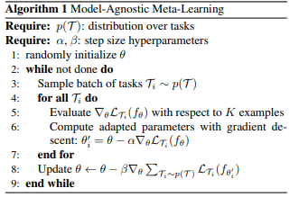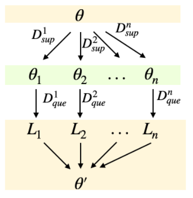which we know is agonistic of what model $f$ we picked.

so that essentially we update $\theta \to \theta’$, where the intermediate $\theta_i$ for each task will be only used for computing the loss for $\theta$ and updating it.
since $\theta_i$ comes from computing task loss $\mathcal{L}i$ and doing $\nabla{\theta_i}\mathcal{L}_i$, and the final $\mathcal{L}(\theta)$ will depend on $\theta_i$, we essentially would need to compute Hessian of $\nabla^2_{\theta_i} \mathcal{L}_i$ when we update $\theta \to \theta’$. This is computationally expensive, and hence we had work such as the Amazon’s Reptile system that approximates the hessian and saves compute power.
resource https://arxiv.org/pdf/1703.03400.pdf

Metric-Based Network

The most notable example of this is the Siamese network, which has the generic task of classifing whether if the two images are the same.

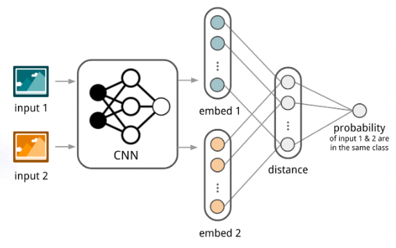
however, the difference with normal training is:

the two input image could come from any domain, e.g. kid’s drawings, signatures, facial photographs, etc.
The idea of this network is to use a shared CNN backbone to get an embedding, then then compute probability by looking at the distance, so that the shared CNN backbone in the middle is generalizable.

In general, metric-based network aims at training a network that can produce good embeddings for a sample in a new domain (haven’t seen in training).

with few-shots, then $K$ samples for each class in the domain

Some other networks should should already know from the Deep Learning course notes:

Matching Network

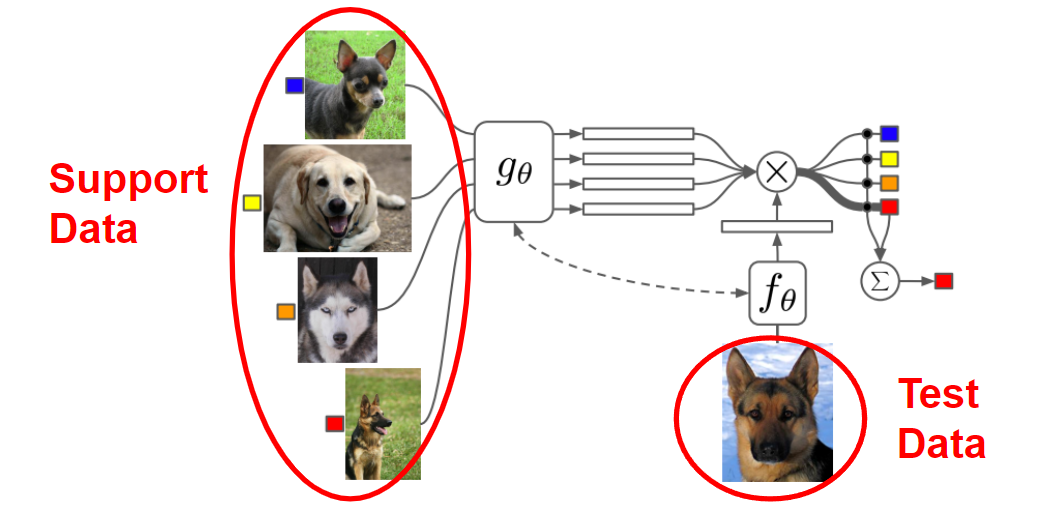
which basically creates an embedding for each input $x_i$, then for the new test sample $x_q$:
\[\hat{y} = \sum_{i}a(x_i,x_q)y_i\]
basically predicting by a weighted average.
Prototypical Network

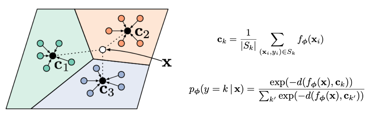
which basically produces a class prototype vector $c_k$, and then for the new sample $x$ classify the class by looking at the distance between its embedding $f_\phi(x)$ and the class vectors $c_k$

Basically they all tend to learn a metric/embedding to produce a good latent space representation of the class.

Applications in NLP

How do we apply the idea of meta-learning in NLP applications?

Meta Leanring for Dialog

Consider the task of

building a dialog system in domain $A, B, C$
training data of dialogs are in domain $A,E,D,F$
preparing a model $M$ that would work not only in $A,B,C$, but perhaps new domains as well

Then essentially it becomes learning a model $M$ that performs well given a few-shot learning samples. Hence we consider utilizing MAML algorithm mentioned above:

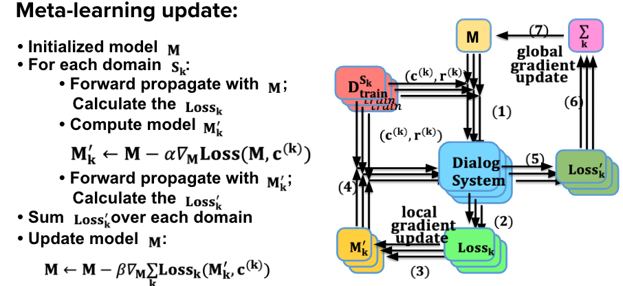
where

$M_k’$ are the temporary models with weights $\theta_k$
The aim is to update $M$ with $\theta \to \theta’$, such that the final $\theta^*$ would work well under few-shot learning

The performance comparision:

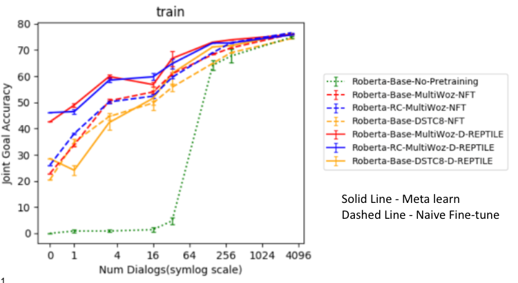
where when the dialog system is trained with meta-learing is is better than just fine-tuning the model to another task

Meta Learning for Machine Translatoin

As mentioned before, it is common to have a MT task that, given a few samples of translating from language $A$ to language $B$, we want it to work even if our training data only contained $C\to D, A\to C, D\to F$, etc.

Graphically, the comparision between Meta-learning and other methods mentioend above is:

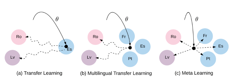
so that:

for transfer learning, we want to start with $\theta$ that works best in one domain and then move to others
for meta learning, you want to get $\theta$ such that it works best at adapation (in all directions)

Meta In Context Learning

Some research has found that

(Large) Language models are few-shot learners

basically they seem to work well with few-shot even if the training procedure is just masked language/whatever that is used normally for a language model training

An example in practice is GPT 3. GPT 3 has huge parameters, and is trained on huge text data.

hard to fit in normal school GPUs
also hard to fine-tune as the model is huge

Therefore a new procedure is needed for few-shot “training”

normally you would imagine we update $\theta$ per step with each new (few-shot) traing data
but as that is intractable, we can just dump all the examples along with the query as input

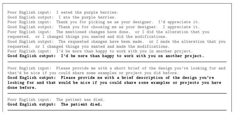
where:

the grey ones are the few-shot examples, the black texts are the machines’ output
so that essentially it is few shot learning without updating weights

How does that even work? As we have transformers in the model:

the model not only attends to the input, it also attends to the context
therefore, we expect models to use the attention mechanism to understand the few-shot

In Context Tuning

Recent results shown that, given that in-context learning works, we can also do the following (for smaller models such as GPT2):

instead of doing one step update for the intermediate weights $\theta_i$ in MAML
we put all the task $T_i$ as a single input with context and fine-tune $\theta \to \theta’$ directly

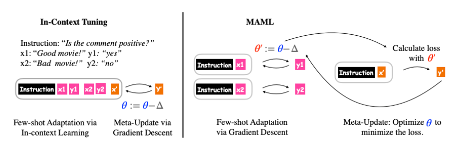
so that essentially:

it is fine-tuning but the training set is a concatenation of support set and query set
since it is a concatenation, the problem becomes memory constraint.
such an update method is also model agnostic

Bias in NLP

Related to ethics and safety of NLP models. Consider cases where:

Language models on Job description preferers/assigns better competency for male engineers over females
Products such as Amazon Alexa outputting racist texts (just for example)

Therefore, in this section we will talk about some methods on

how to detect biases
- https://arxiv.org/abs/1608.07187
- https://www.aclweb.org/anthology/N19-1063.pdf
how do to de-biasing
- https://www.aclweb.org/anthology/N19-1061.pdf

Bias in Word Embeddings

In machine learning, essentially bias refers to prior information/the priors. The are problematic when such information is derived from aspects of human culture known to lead to harmful behavior

e.g. Word2Vec: “Man is to computer programmer as woman is to homemaker.”

Just as there are tests to measure implicit bias in humans, there can be parallel test to measure bias in machine, and today we mostly do this by looking at the learnt embeddings. Here, we can consider word level embeddings.

Word embedding representations, in addition to encoding semantic meaning, also encode semantic analogy.

using that, we can analyze whether if certain words are gender/race neutral, for example.

Implicit Association Test and WEAT

A famous test by Harvard is useful to measure biases in Human: the Implicit Association Test

The IAT measures the strength of associations between concepts (e.g., black people, gay people) and evaluations (e.g., good, bad) or stereotypes (e.g., athletic, clumsy). The main idea is that making a response is easier when closely related items share the same response key.

Some useful word pairs we will discuss are:

Flowers, insects - pleasant, unpleasant
European American Names, African American Names - pleasant, unpleasant
Female names, male names - family, career
etc.

This essentially inspires how we can perform a similar task for word embeddings

Word-Embedding Association Test (WEAT) essentially computes such association of concepts with cosine similarity of the embeddings, and was able to replicate the stereotypes found in the IAT tests.

The details are formalized as follows. Consider:

two sets of target words $X$ (e.g., programmer, engineer, scientist; and nurse, teacher, librarian)
two sets of attribute words $Y$ (e.g., man, male; and woman, female).
The null hypothesis is that there is no difference between the two sets of target words in terms of their relative similarity to the two sets of attribute words.
The permutation test measures the (un)likelihood of the null hypothesis by computing the probability that a random permutation of the attribute words would produce the observed (or greater) difference in sample means.

Therefore, the test statics of the differential association of the two sets of target words (so that it is highest when the two groups have a different association, e.g. $X \to A$ and $Y \to B$) computes:

\[s(X,Y,A,B) = \sum_{x \in X}s(x,A,B) - \sum_{y \in Y}s(y,A,B)\]

where

\[s(w,A,B) = \text{mean}_{a \in A} \cos(\vec{w},\vec{a})-\text{mean}_{b \in B} \cos(\vec{w},\vec{b})\]

essentially measure the association of words to attributes in $A$ v.s. attributes in $B$. So that this is large when the word $\vec{w}$ is biased towards a particular group of attributes.

From this we can also formulate the permutation test and the effective size (to reject the null hypothesis), for which we will skip here but can be found on https://www.science.org/doi/10.1126/science.aal4230

Example of Biases Found in Word Embeddings (such as Word2Vec)

Racial Bias: African American names v.s. European American names

Target	Attributes

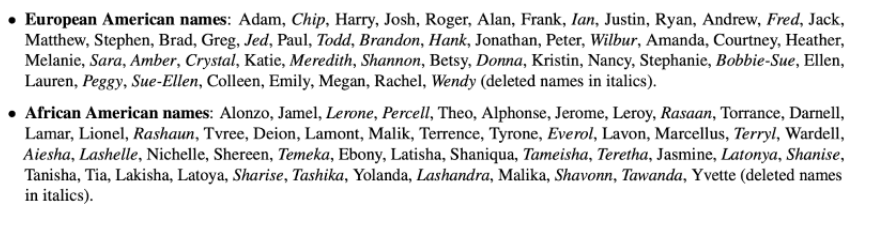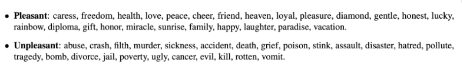Gender Bias: Females are more associated with family, men with careers

Target	Attributes

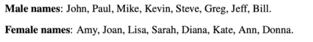Gender Bias: Female terms more associated with arts, male terms with mathematics

Target	Attributes

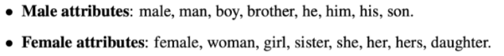Where does those bias come from? It is basically learnt from current world statistics (which is biased). For example

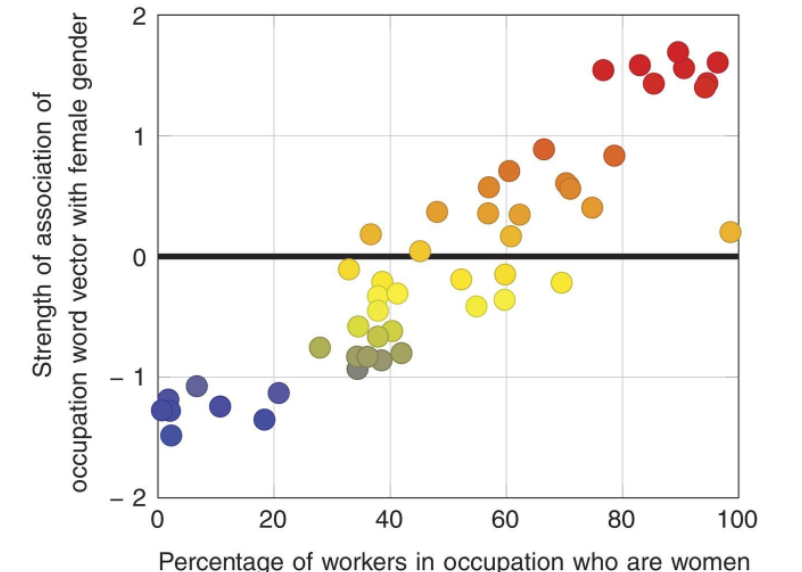
where we see that:

it learns to output a high similarity score for occupations where there are more women
but we want it to learn those occupations to be gender neutral even if this is the reality

Effect of Bias on NLP

As we know that many laguage models are trained on a huge amount of text:

easily pick up biases from old documents/books, for example
different languages might have different associations/biases

Sapir-Whorf hypothesis: “real world” is to a large extent unconsciously built up on the language habits of the group

Therefore, together with biases thise produces problems such as:

MT translation:
- Chinese speeches do not distinguish between he/she
- to translate to English, we need he/she
- but we should not disambiguate those based on biases!
Dialog
- e.g. implicitly using a pronoun such as “he” when referring to boss?

Both of which not only relates to biases in word level embeddings, but also perhaps bias in sentence level embeddings!

Bias in Sentence Embeddings

The idea is the same as WEAT, where we want to know if the same bias exist for sentence embeddings. The only difference is:

we have sentences, hence added context
the target and the attribute sets are sets of sentences

SEAT: Sentence Encoder Association Test. This basically does the same procedure as WEAT where you can:

form a sentence from words by simple templates where the word has been inserted: “This is a <word>”.

this is often used to convert word attributes to sentence attributes.

or if you have sentences to tests as targets, use them directly

For example:

Target	Attributes

The upshot is that the same biases still exists.

ABW and Double Bind

Two traditional biases that were studied are:

ABW: “angry black woman” stereotype, basically black women are portrayed as loud, angry and imposing
Double Bind: women in professional settings treated with disadvantage v.s. man
- If women succeed in a male dominated job, they are perceived less likeable and more hostile than similarly performing men
- If success not clear, they are perceived less competent and achievement oriented than men

ABW Study:

Target: Black and white women names
Attributes: adjectives presented in Collins and their antonyms

Double Bind Study (likeable):

Targets: male/female names. “Kathy is an engineer with superior technical skills”
Attributes: likable and non-hostile terms: “the engineer is nice”

Double Bind Study (success):

Targets: “Kathy is an engineer”
Attributes: competent/achievement-oriented terms: “The engineer is high performing.”

Results:

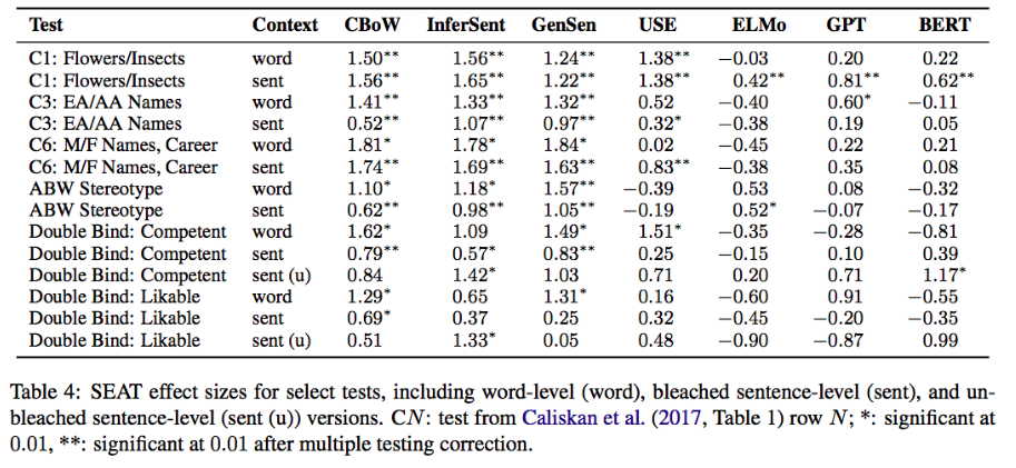
Hence we see that:

for word level, you can basically pass in the word itself as a sentence and take that as the mebdding
ELMo, GPT, and BERT seem to have bias when used with sentence level but not when they are doing on a word level
however, there are discrepancies as many results does not seem to agree even with same p-values

The conclusion is that:

SEAT can confirm that bias exists
Cosine similarity may not be a suitable model of representational similarity in recent models (e.g., BERT)

Debiasing

Is it possible to remove the bias that is clearly present in real life statistics?

It is still under active research, but we do have some approaches

HARD-DEBIASED: remove the bias after training by post-processing
GN-GLOVE: use a loss function during training that aims to reduce bias

However, the quick conclusion is that even those does remove surface level bias (the word embedding itself may not be biased), it does not reduce hidden biases such as “doctor” and “boss” having a similar embedding v.s. “nurse” and “teacher”

De-bias via Post Processing

Given a word $\vec{w}$, we can define its gender bias (for example) by its projection on the “gender direction”:

\[\vec{w} \cdot (\vec{he}-\vec{she})\]

where $(\vec{he}-\vec{she})$ would be the gender direction. We can compute this in a more robust way by taking

taking 10 pairs of words that surely have gender differences
take the principle components of the 10 pairs

Then, when we have this gender direction

for all words that should not be inherently gendered
Zero the gender projection for each word

De-bias via Loss Function

Instead of removing/post processing the embedding, consider having loss such that

words in different groups to differ in last coordinate (as we know they exist in our data)

neutral gender words to be orthogonal

Then essentially:

Train debiased word embeddings from scratch
Change the loss function for Glove as mentioned above
- so essentially concentrate gender information in last coordinate
Once done, remove the last coordinate

Hidden Bias via Clustering

Essentialy the paper https://www.aclweb.org/anthology/N19-1061.pdf claims that the above does not remove the biases.

They manage to hide the bias in their neighborhood relationship, even if their similarity to gender is removed.

most word pairs maintain their previous similarity, despite their change in relation to the gender direction

Consider

taking the most biased words in the vocabulary according to the original bias
- 500 male biased, 500 female biased
Cluster into 2 clusters using k-means
- compare the result before de-biasing and after de-biasing

Results:

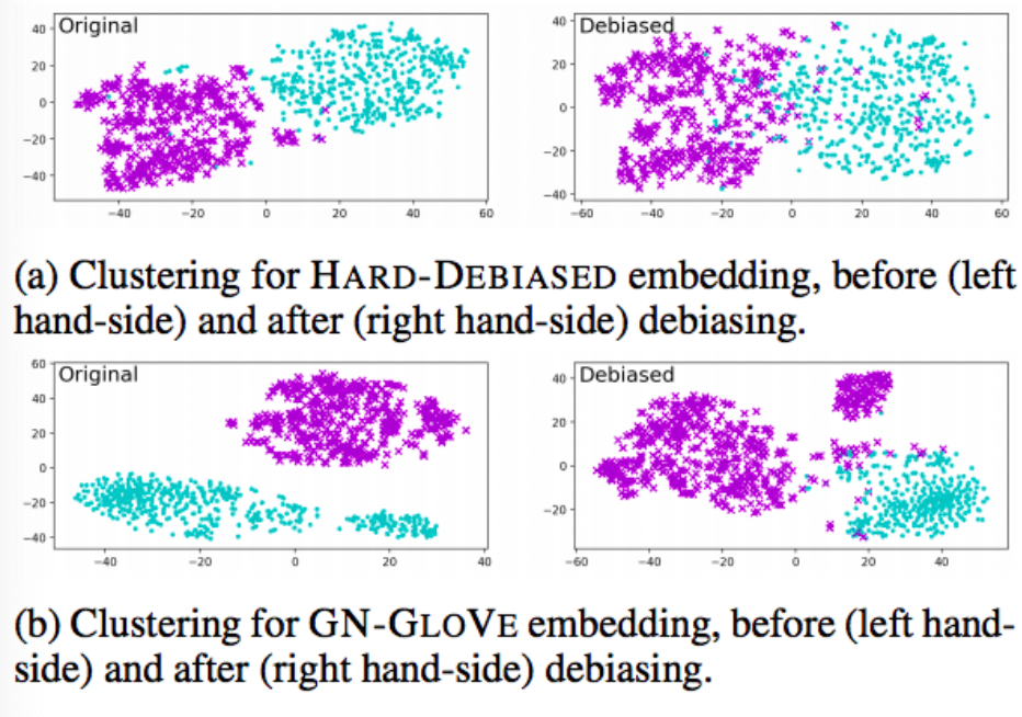
where we see that

Bias still manifested by the word being close to socially-marked feminine words
i.e. although they are hiding their bias w.r.t gender, but their neighbor relationship is still apparent

Therefore, this introduces a new mechanism for measuring bias: % male/female socially-biased words among the k nearest neighbors of the target word.

Another intuitive metric could be:

given 5000 most biased words according to original experiments
Train an SVM on 1000 random sample, predict gender for remaining 4000

So that if words embeddings still have biases, then models such as SVM will not be able to distinguish. However, in reality:

Hard-debiased: 88.8% accuracy vs 98.25% accuracy with non-debiased version
GN-Glove: 96.53% accuracy vs. 98.65% accuracy with non-debiased version

so, again those biases are hidden somewhere in the embeddings.

Idea: using GAN to perhaps remove the bias.