COMS4732 Computer Vision II
- Introduction
- Convolution
- Fourier Transform
- Machine Learning
- Object Recognition
- Video Recognition
- Object Tracking
- Interpretability
- Self-Supervised Learning
- Synthesis
- Ethics and Bias
- Vision and Sound
- Vision and Language
- 3D Vision
- Final Exam
Introduction
What is vision?
Applications
One very important application is Biometrics
- how FaceID works!
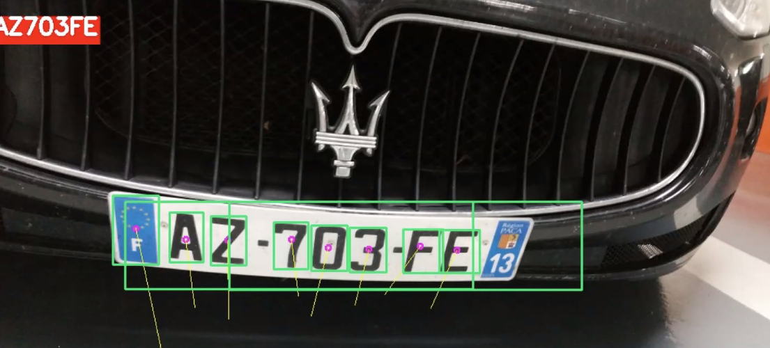
Another would be Optical Character Recognition
Gaming with VR: recognize your body poses:
- recognize fine details about your movements

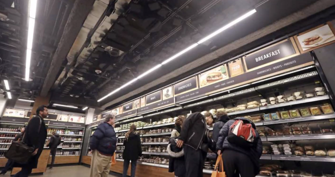
Recently there has been application in shopping
-
as a customer, you can grab whatever you want, and you will be charged by Amazon
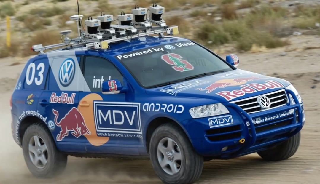
Last but not least, self-driving cars
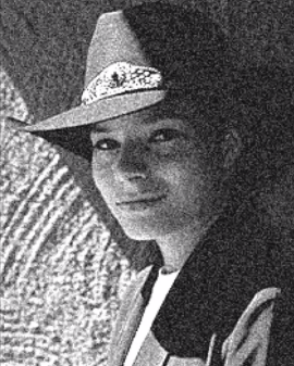
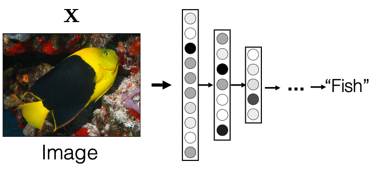
Perceiving Images
Basically the input of an image would be
| What We See | What Computer Sees |
|---|---|
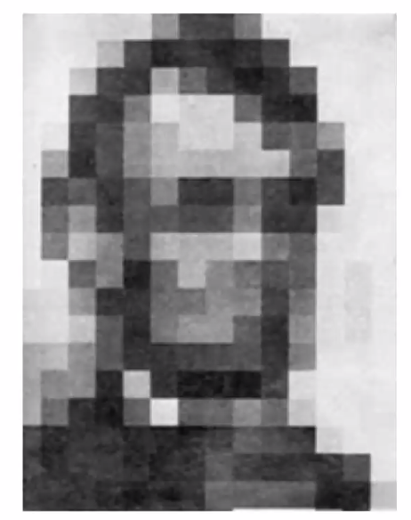 |
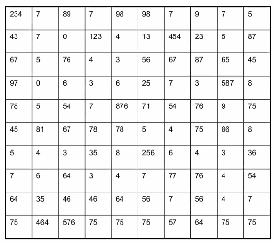 |
which hints at the why computer vision is difficult.
-
other factors that could make it more complicated is the lighting, which can change the picture
-
object occlusion, an object will be partially blocked
-
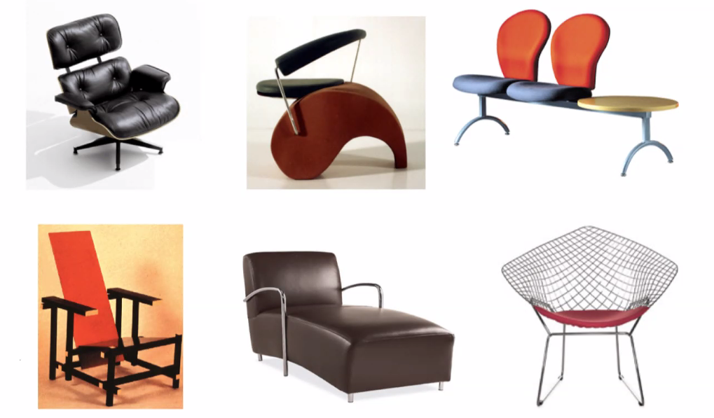
class variation: objects can have various shapes. What is a chair?
-
clutter and camouflage: we are able to see through camouflage
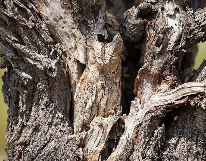
so that we can see there is an owl, but computer vision systems would struggle here.
In general, there is often no correct answer for computer vision!
Evolution of Vision
Before the Cambrian explosions, there were only about 4 species (worm-like) on Earth. However, after the explosion:
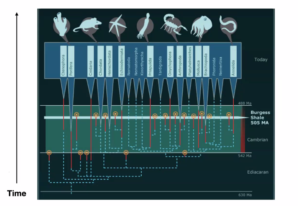
some theories to
- “In the blink of an eye”: The Cambrian Explosion is trigged by the sudden evolution of vision, which set off an evolutionary arms race where animals either evolved or died.
- our vision has evolved for more than 200 million years. Now let the computer do it.
What don’t we just build a brain?
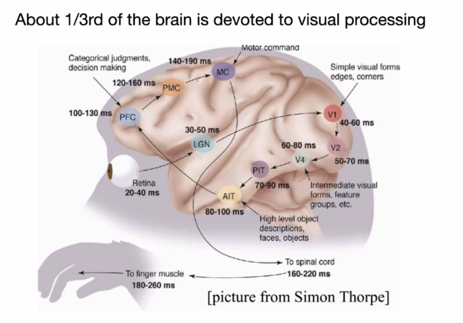
where we start the loop from our retina:
- starting from PFC it is related to other stuff.
- but even until today, we are still not sure how brain works.
Additionally, there is a difference in datasets
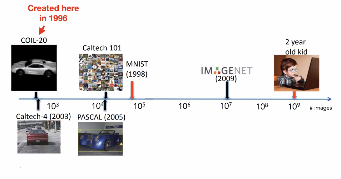
notice that what a 2 year-old child have seen would have been much more than the best dset we have now.
Syllabus
Because the course is large, there will be no exceptions at all
Topics: we do NOT assume prior knowledge in computer vision and machine learning
Format: Hybrid
- so Zoom is allowed
- every lecture will be recorded
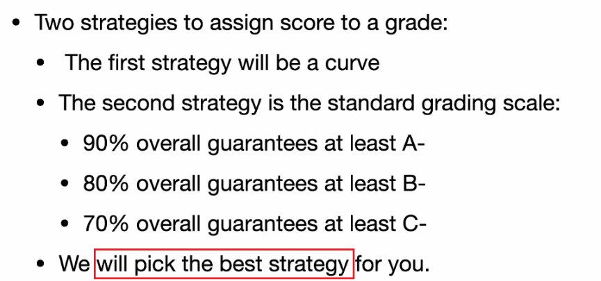
Grading
- Homework 0: 5% (self-assessment, should be easy)
- Homework 1 through 5: 10% each
- Final Quiz: 45% (written)
Homework: outlines
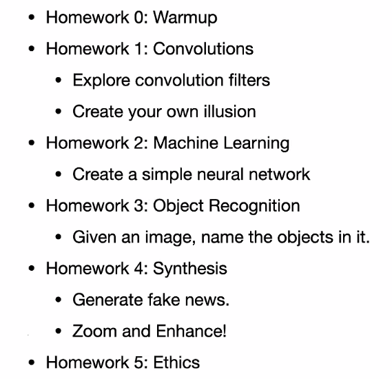
- usually it will be 2 weeks for each homework
- probably hand in via Gradescope
- collaborations will be allowed, but need to disclose
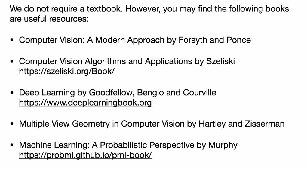
Useful Resources
OH
- will be online
Optical Illusions
Below are some interesting illusions
| Illusion | Your Brain |
|---|---|
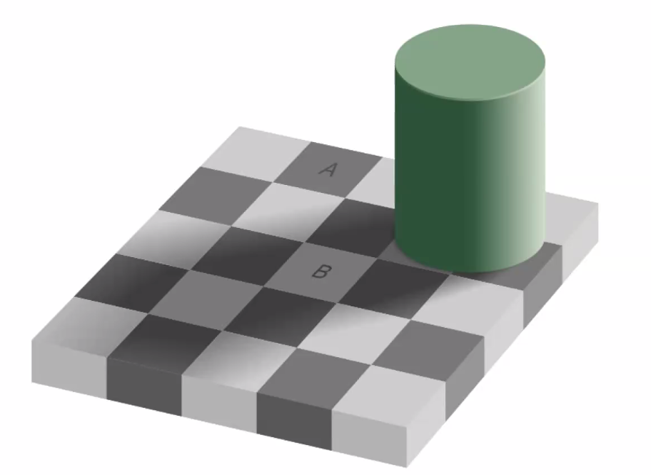 |
You brain “factors” out the fact that there is a shadow, which automatically made a block $B$ seem lighter than $A$. (How can your computer vision do this if they have the same RGB?) |
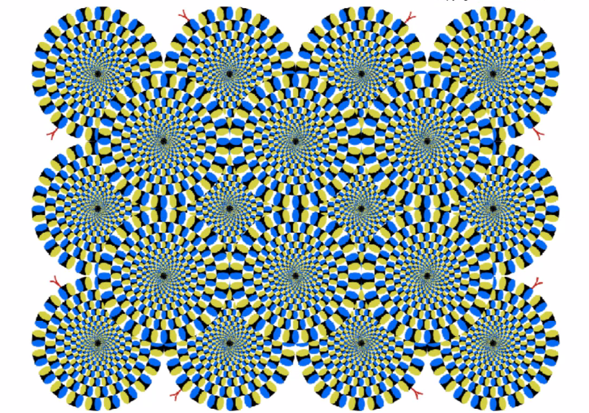 |
Some explanation of this talks about that you see them “moving” because your neurons overloaded. |
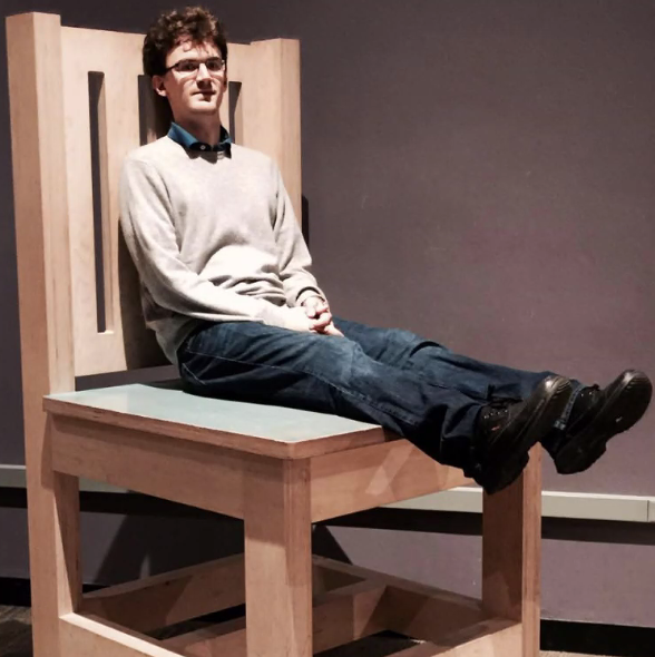 |
Ambiguities our brain resolve pretty fast: a big chair instead of a small person |
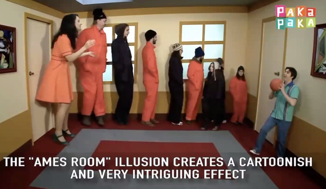 |
Makes you think people shrunk in size. But actually this is how it happened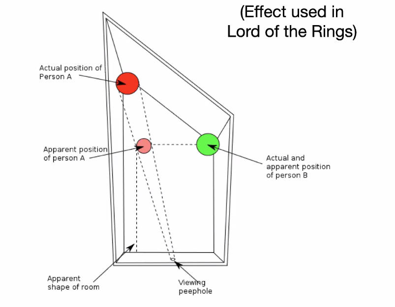 |
in short:
- our brain “automatically fill in things” that are not there - hard part of perception
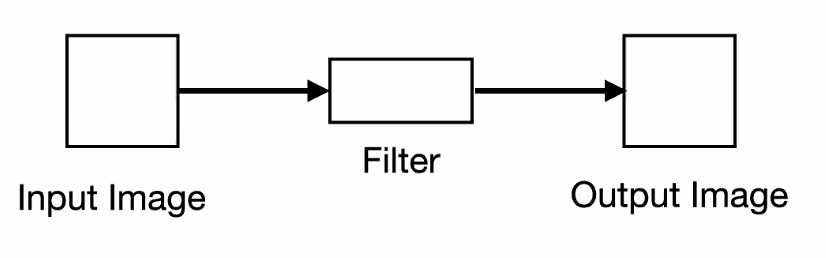
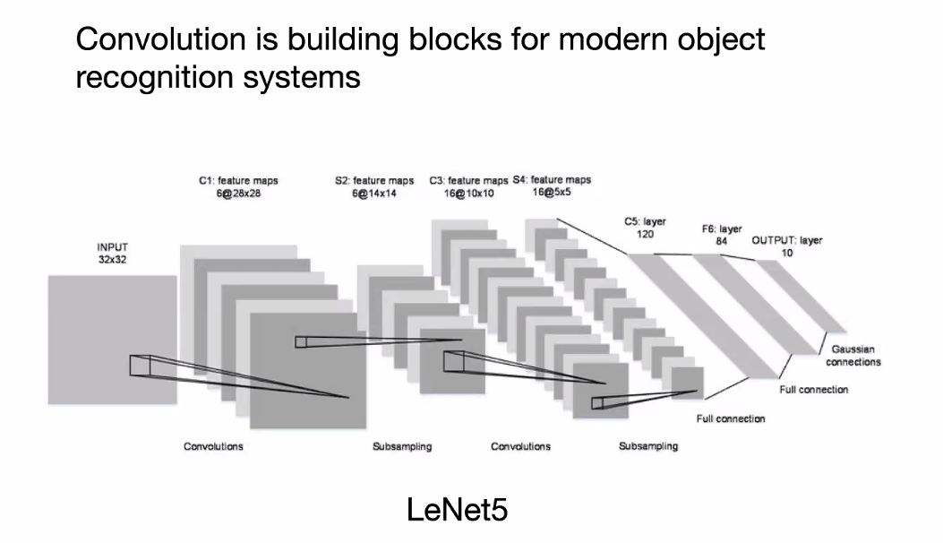
Convolution
The idea is that we want to de preprocessing of the image, such that:
- we can “denoise” an image.
- highlight edges (taking gradient)
- etc
using a linear kernel/filter, which essentially are using weighted sums of pixel values using different patterns of weights to find different image patterns. Despite its simplicity, this process is extremely useful.
For instance, when you take a photo at night, there is little light hence it would capture a lot of noise
Intuition
One way to suppress noise would be to:
- take many photos and take average
- how do we “take an average” even if we only have one photo?
One way to think about this, is that we can first treat each image as a “function”
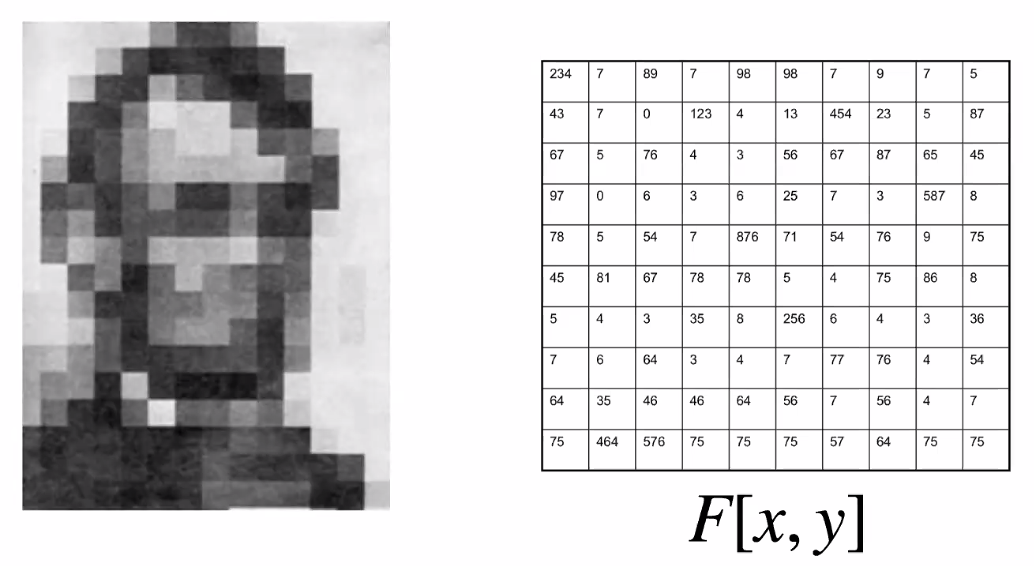
where:
- as a function, the image maps a coordinate $(x,y)$ to intensity $[0,255]$
- (in some other cases, thinking of this as a matrix would work)
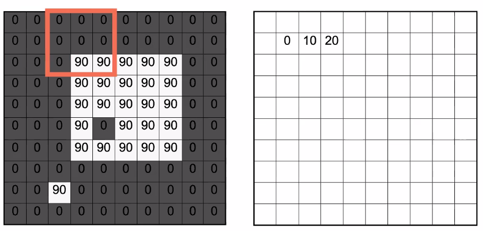
Then, then, you can take a moving average:
| Sliding Through | Output |
|---|---|
 |
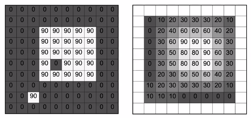 |
when we finish, notice that:
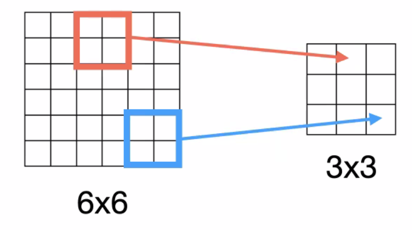
- the next effect is that it “blurs” or “smooths” the image out
- the output has a smaller size than the input. This is because there are $(n-3+1)^2$ unique positions for putting the $3\times 3$ kernel.
Linear Filter
The above can also be thought of as:
In general, we will be looking at linear filters, which has to satisfy the following
-
$\text{filter}( \text{im},f_1 +f_2) = \text{filter}( \text{im},f_1) + \text{filter}( \text{im},f_2)$
-
$f_1,f_2$ are filters/kernels. The function is the process of applying them to the image.
- output of sum of filters is the same as sum of output of filters $f((a+b)x)=f(ax)+f(bx)$
- since filters can also be seen as “images”: output of the sum of two images is the same as the sum of the outputs obtained for the images separately.
-
-
$C\cdot \text{filter}( \text{im},f_1) = \text{filter}( \text{im},C\dot f_1)$
- multiplied by a constant
And you can think of this as linear algebra
- most of the convolutions operations are linear by construction
Convolution Filter
Kernel/Filter: The pattern of weights used for a linear filter is usually referred to as the kernel/the filter
The process of applying the filter is usually referred to as convolution.
For instance, we can do a running average by the following convolution:
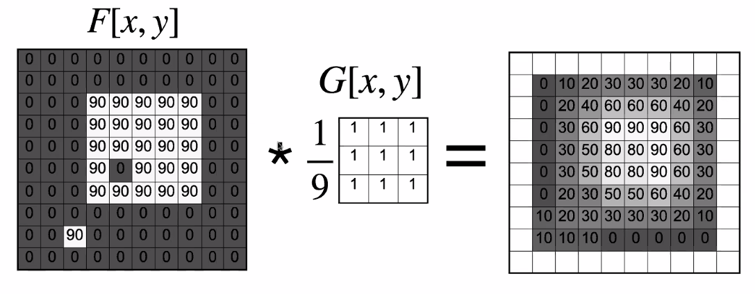
where:
- $*$ is often a symbol used for convolving
- essentially it is about taking $G$ , then taking sum of element-wise product with a $3\times 3$ region in $F$
- This is the same as moving average we had. But notice that we needed $1/9$ in front:
- In reality, we also want to make sure that the output is still a valid image. Hence we need to be careful that the output intensity value does not exceed $255$, for instance.
Formally, convolution is defined as:
\[(f * g)[x,y] = \sum_{i,j} f[x-i,y-j]g[i,j]\]where
-
$(f * g)[x,y]$ means $f$ convolves with $g$, which is a function of coordinate $x,y$. Outputs the intensity at $x,y$.
-
For a $3\times 3$ kernel, we would set $i \in [0,2], j \in [0,2]$ and output to the top right instead of center.
-
notice that the minus sign is intended, so that we are flipping the filter:
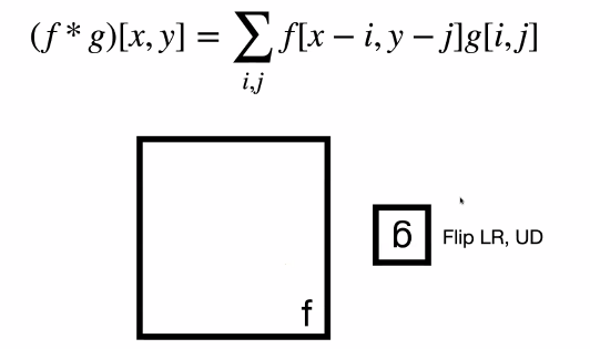
where:
- the only purpose of flipping is that it makes the math easier later on
- increasing index in $g$ but doing decreasing for $f$.
- therefore, you need to flip the filter upside down, and then right to left
- when you code it, however, often you will just have
+sign.
Note that if the filter is symmetric, then flipping doesn’t matter.
- However, if the filter is not symmetric, (most people) just don’t flip it either way. So it depends.
If you use the $+$ instead, it is called a cross-correlation operation
\[(f * g)[x,y] = \sum_{i,j} f[x+i,y+j]g[i,j]\]which is also denoted as:
\[f \otimes g\]which does not have all the nice properties like convolution just due to that sign.
For instance: convolution examples
Identity transformation:
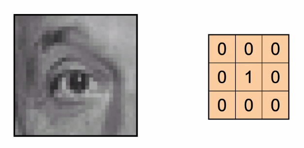
- basically It will output the same image (but contracted by 1)
Translation
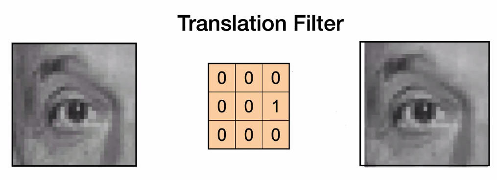
-
where it shifts to the right because we had the minus sign. In essence, we need to flip the convolutional kernel upside down and right to left, which becomes this:
hence it is in fact shifted to the right
Nonlinear Kernel
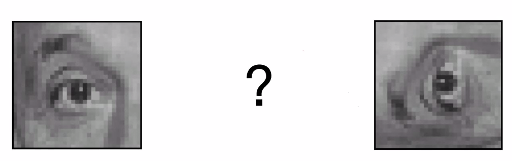
where notice that no such convolution kernel exist, because:
- this is not a linear operation!
- for convolution kernel to work, we needed to **treat everything/pixel identically (from its neighbors) **. However, a rotation doesn’t work like this (e.g. consider the treatment of the pixel in the center and the pixel far away from the center on the LHS image)
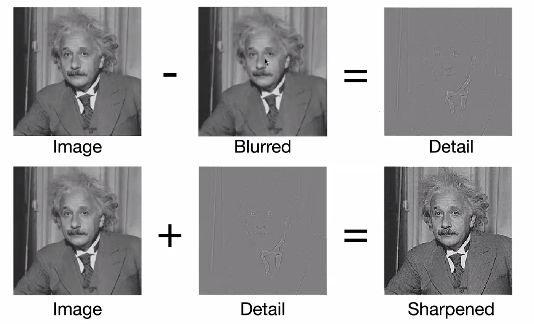
Sharpening
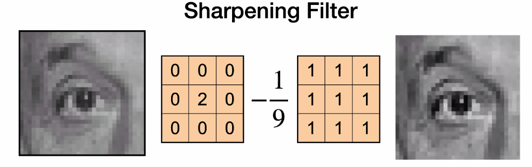
where:
-
sharpening actually increases the noise
- multiply by $2$ is like brightening
- subtracting a blurred image = subtracting removed noise
-
so it turns out that our eyes think “adding noise” makes the photo looks sharper
Convolution Properties
The operation $*$ has the following property:
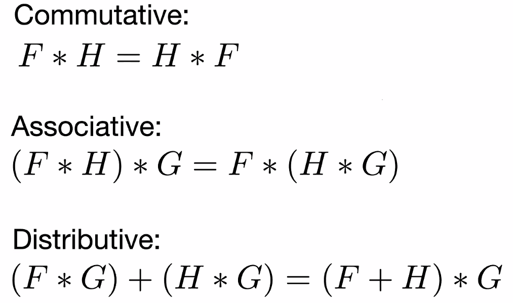
those can be proved with the minus sign in our definition, which switching to plus sign might make things break. $F,G,H$ are all filters/kernels, so remember that $F * G$ means, .e.g having image $F$ convolve with filter $G$
- commutative/associative: order of convolution does not matter. You can apply $F$ then $G$, or $G$ then $F$
- distributive: same as linearity of kernels
Note
- you kind of have to ignore the fact that different sizes of image/filter produces a different border
- those are useful because it makes your code runs faster
Additionally, we also know that
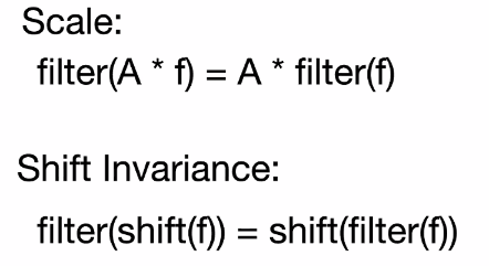
which makes sense since a linear convolution treats each pixel the same/”same weights from neighbors”.
Gaussian Filter
Now, let us reconsider the task of blurring an image: we can blur the image by “creating multiple copies of the image”, dis-align them and add them up:
| Box Filter | Gaussian Filter |
|---|---|
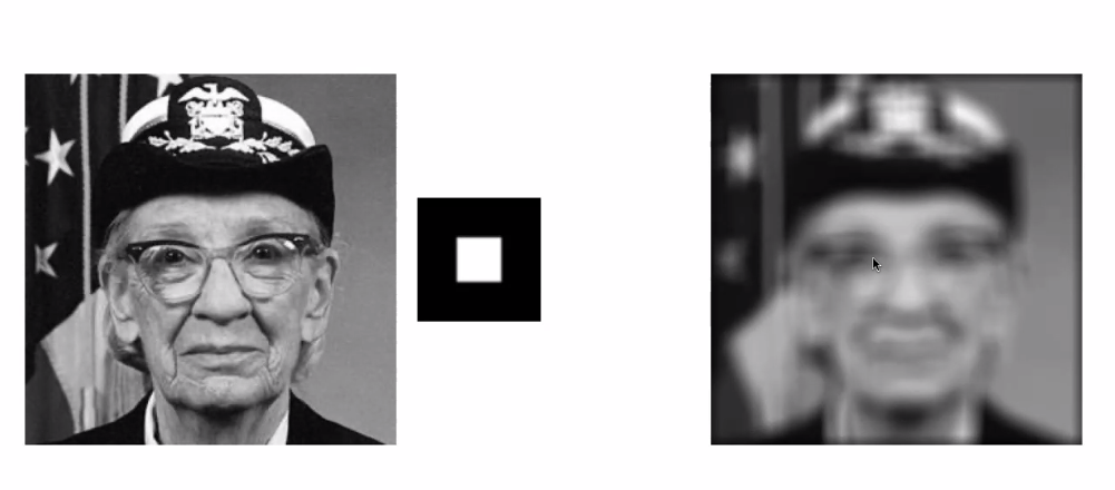 |
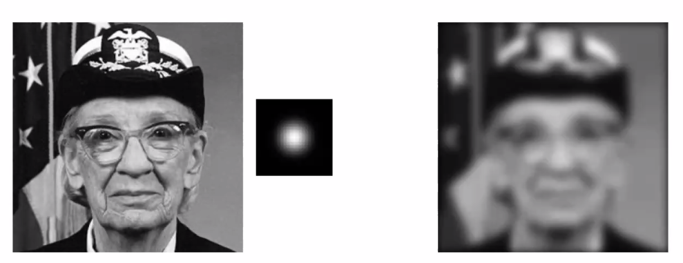 |
where in both cases, we have blurred/smoothened the image
- black means 0, white means 1, and this white box is larger than $1 \times 1$ in size.
- smoothing: suppresses noise by enforcing the requirement that pixels should look like their neighbors
- the Gaussian one does indeed is more visually appealing
More mathematically, the Gaussian is a multivariate Gaussian but having identity as covariance: i.e. the two variables are independent:
\[G_\sigma = \frac{1}{2\pi \sigma^2} \exp({ - \frac{x^2 + y^2}{2\sigma^2}})\]where $x,y$ are coordinates, and an example output looks like:
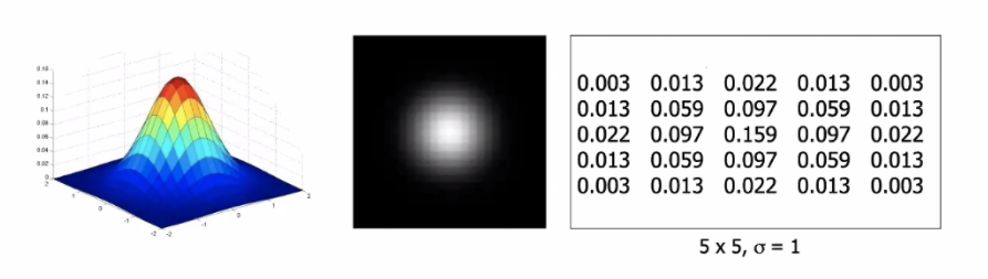
recall that Gaussian also has the nice property that they sum up to 1.
- notice that it is symmetric. This is enforced.
- yet since it is a Gaussian, we can also control its parameters $\sigma$, which determines the extent of smoothing
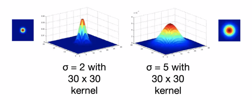
so that:
- more spread out gives more blur
For instance:
| Slow Sigma | High Sigma | |
|---|---|---|
 |
 |
 |
Computation Complexity
For having an image of $n\times n$ doing a convolution of $m \times m$ kernel/filter:
\[O(n^2 m^2)\]where we assumed that there are paddings done, so the output is the same size as input.
- For each single pixel, we need to do $m \times m$ work
- Since we have $n \times n$ pixels, we needed to $n^2 m^2$
- this is very expensive!
But we can speed this up in some cases. Consider separating the Gaussian filter into 2:
\[G_\sigma = \frac{1}{2\pi \sigma^2} \exp({ - \frac{x^2 + y^2}{2\sigma^2}}) = \left[ \frac{1}{\sqrt{2\pi }\sigma} \exp({ - \frac{x^2 }{2\sigma^2}}) \right]\left[ \frac{1}{\sqrt{2\pi} \sigma} \exp({ - \frac{y^2}{2\sigma^2}}) \right]\]Therefore, since we know that if we have two filters $g,h$, and an image $f$, associativity says:
\[f * (g * h) = (f*g)*h\]Therefore
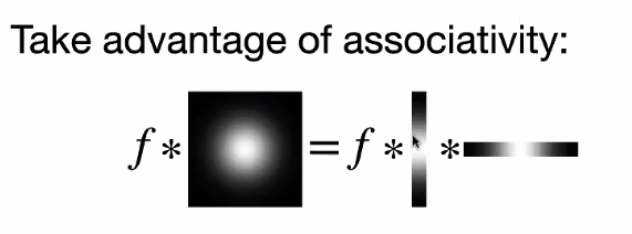
(technically, we are saying the following)
\[f * g = f * (g_v \times g_h)= (f* g_v) * g_h\]Then, since $G_\sigma$ can be separated into two filters of smaller dimension:
\[O(n^2 m)\]now for each pixel, we only needed to do $m$ work/look at $m$ neighbors.
- technically you do it twice, so $2n^2m$, but $2$ is ignored.
- this only works in special cases.
Human Visual System
In fact, one stage our vision system also does convolution
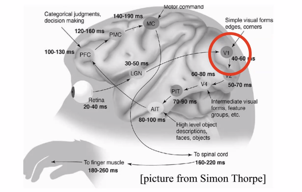
- $V1$ is doing convolution.
Experiments have been done on cats, and show that the kernel they are using looks like the following
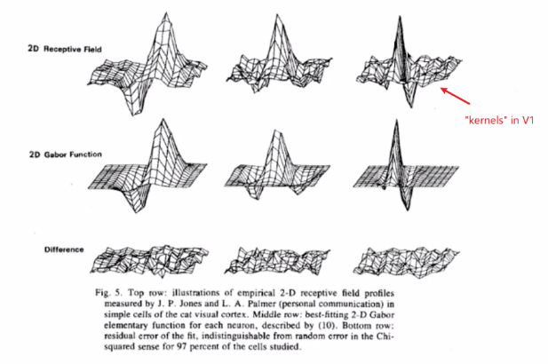
where:
- to simulate the kernels in cat, we have those Gabor’s filter
Gabor Filters
Gabor filters are defined by:
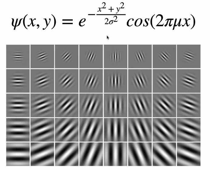
interestingly:
- it seems that convolutional NN also returned a similar filter
- it turns out this can do edge detection
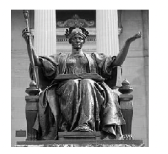
Image Gradients
Now, we want to consider the problem of identifying edges in a picture, which is part of an important process in identifying objects.
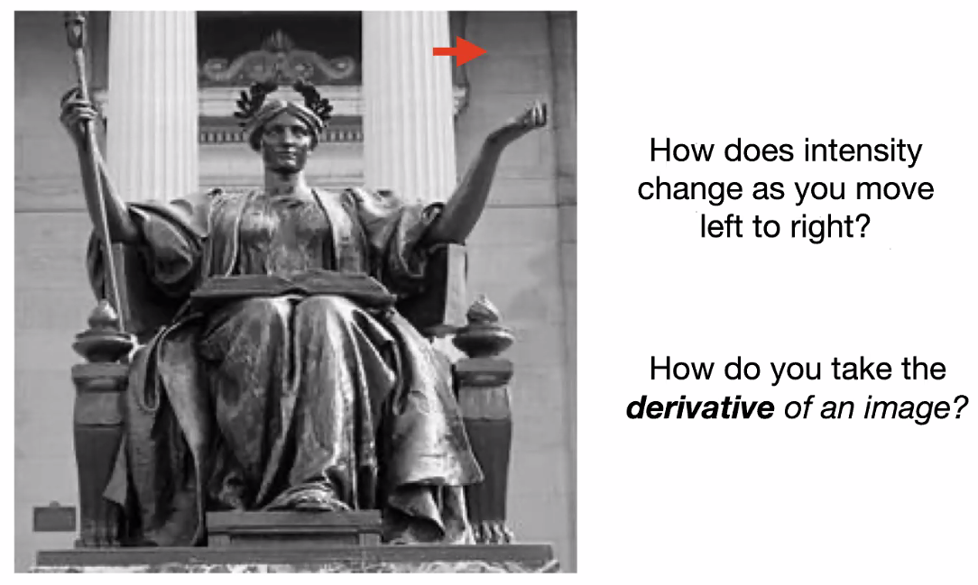
Consider looking at the red arrow. We are interested in how does the intensity change
-
when we moved across the pillar, it seems that intensity changed dramatically!
-
so we want to compute the “derivatives”
We know that
\[\frac{\partial f}{\partial x} = \lim_{\epsilon \to 0} \frac{f(x + \epsilon ,y)-f(x - \epsilon ,y)}{\epsilon}\]but since the smallest unit is a pixel:
\[\frac{\partial f}{\partial x} \approx f(x+1,j) - f(x-1,j)\]Therefore, we basically have the following:
- $\partial f/ \partial x$: using $[-1,0,1]$ or $[-1,1]$ as kernel
- $\partial f/ \partial y$: using $[-1,0,1]^T$ or $[-1,1]^T$ as kernel
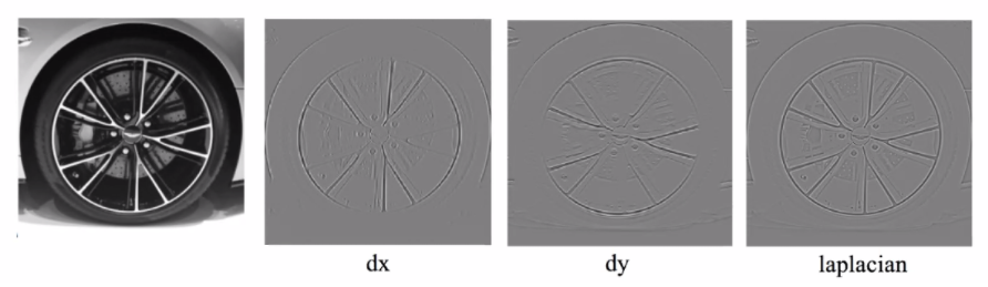
Result:
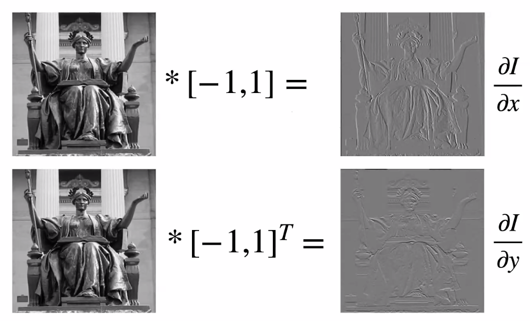
where we see:
-
the $\partial x$ shows how images change when we move in $x$-direction. Hence we see the texture of the pillars on the RHS. But if we do $\partial y$, they disappear.
- if we want to be more “exact”: $0.5[-1,0,1]$ since the step size is $2$ pixels
- technically the signs are “backwards” because we need to flip our kernel
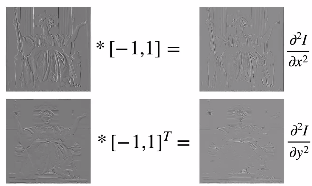
Similarly, we can also compute second derivative from using the first derivative as input:
Edge Detection: Idea
There is no strict “definition of what is edge”, so it is more like a practical trial and error:
- detect edge such that first derivative has a largest change in some region, i.e. second derivative is $0$!
We may care about second derivatives because, usually our image will be noisy:
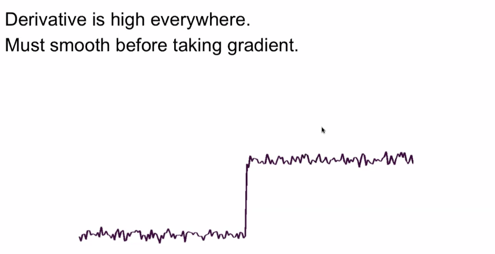
notice that derivatives is high everywhere
- hence we may need to smoothing it first
- then the edges has the larges derivative among them
Therefore, we can do:
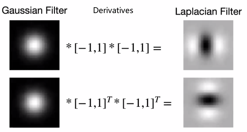
again, we can combine them because:
- convoving with filter 1, then convolve with filter 2 = covolve with (filter 1 convovle filter 2)
- notice that they are all linear filters!
- the Laplacian filter looks similar to the Gabor filter! Detecting the edge!
Note
If you pad an image with $0$ outside (instead of reflection), then essentially you will be adding an extra edge to the image.
- though in a CNN, those could be learnt
Laplacian Filter
The more exact definition of Laplacian filter is:
\[\nabla^2 I = \frac{\partial^2 f}{\partial x^2} + \frac{\partial^2 f}{\partial y^2}\]For instance
where basically:
- edges will get high intensity
Another example, but now we threshold the second derivative:
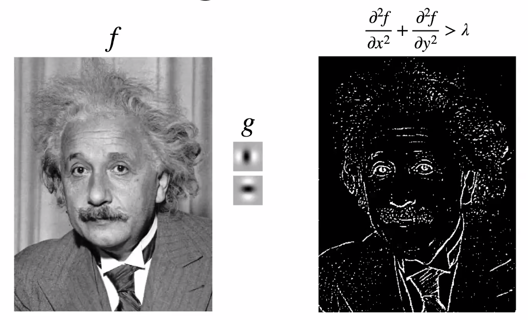
- smaller than $\lambda$ so that changes in gradients are large
Object Detection: Idea
What if we “convolve Einstein with his own eye”: (with the aim of finding the eye)
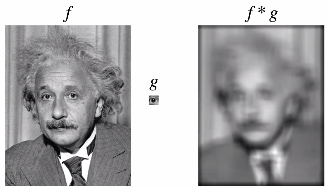
where we see that the results are not that good.
-
in the end, this is where machine learning kicks in, let it figure out what
-
note that the above does not work because, if you think of $f_{ij} * g$ as computing a cosine similarity between vectors as we are doing inner products anyway:
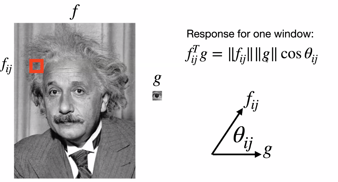
then obviously it does not work.
However, it turns out that we can do the following:
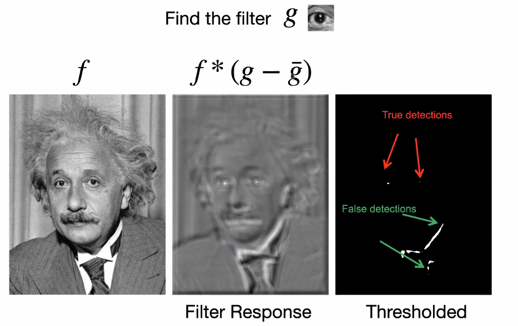
-
so the problem is more like how do we find the right filter.
-
Finally, this task will be one reason why we will be using CNN to learn the filters
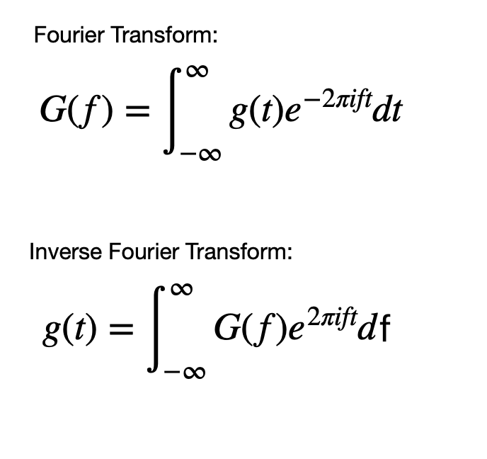
Fourier Transform
The basic idea of Fourier Transform is that any univariate function an be rewritten as a weighted sum of sines and cosines of different frequencies. (recall in PDE)
\[f(x) = a_0 + \sum_{n} a_n \sin (n \pi \frac{x}{L}) + \sum_{n} b_n \cos(n\pi \frac{x}{L})\]An example would be that we can:
| Original | Fourier Series |
|---|---|
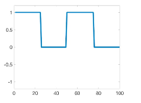 |
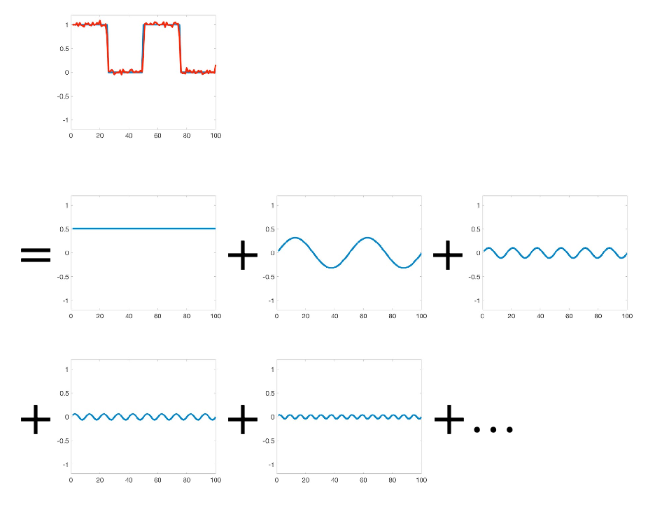 |
If this is true, we can also fourier transform the 2D images as sums:
| Original | Fourier Series |
|---|---|
 |
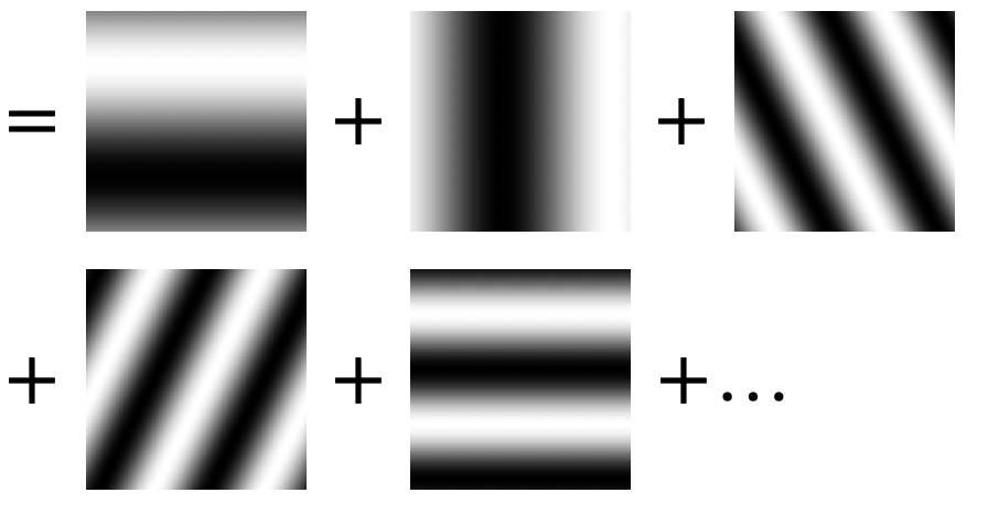 |
where
- we can use this for, e.g. compression, by removing some higher order terms to reduce data but still making the image look reasonbly good.
- now, since the source function is in 2D, fourier transform basically converts it to a sum of 2D waves
- notice that the frequency of the “image” increases. This is basically what happens in higher order frequency terms in FT!
Note
The key idea in this chapter is that images, which can be treated as function $g(x,y)$, can be thought of as a linear combination/sum of waves with different frequencies $u,v$. Such that, in the end it is found that:
- low frequency information usually encapsulates details of the image
- high frequency usually encapsulates noise
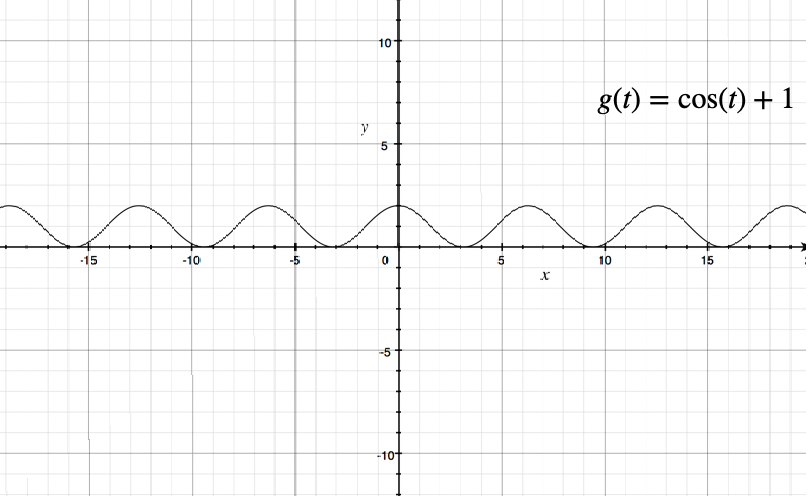
Backgrounds
Recall that for a sinusoid, we have three key parameters to specify a wave
\[g(t) = A \sin(2 \pi ft + \phi) = A \sin (\omega t + \phi)\]where:
-
$A, \phi , f$ are amplitude, phase, freqency respectively.
-
essentially, Fourier transform gets any function to a sum of those waves by telling us what would be the $A_i, \phi_i, f_i$ for each component (technically, Fourier transform is a function when given frequency $f_i$, what will be the amplitude and phase $A_i, \phi_i$)
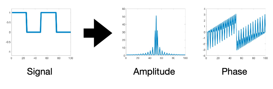
where frequency is encoded in the $x$-axis
- for instance, according to the graph, the decomposition to $f=0$ has $A\approx 55$ and $\phi = 0$
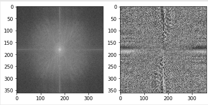
Now, in 2D,
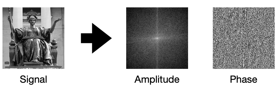
where since our image is in 2D, we will have two axis/two waves: horizontal frequency and vertical frequency.
- typically the coordinate $(0,0)$ will be in the center of the image
- for amplitude graph: black means $0$, white is large
- for phase graph: grey means 0, black means negative, and white means large
- note that fourier series by default generates an infinite amount of waves, yet here we do cut off at certain frequencies
- all those waves are fully specified by $A_i , \phi_i, f_i$, which are all available on the two plots!
Fourier Transform
Aim: the goal of this is to find a procedure, that
- given some signal wave $g(t)$, or $g(x,y)$ if you think of images, and a frequency $f$ of interest
- return $A_f, \phi_f$ being the amplitude and phrase corresponding to that $f$
so essentially tells you the $f$-th term in the fourier series.
Recall that we can we know
\[e^{ift} = \cos (ft) + i \sin (ft)\]Then, if we increase $t$, we will basically find a unit circle
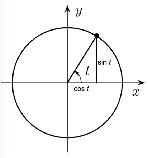
where the vertical component will be $i$. So this could represent a wave!
- e.g. increasing amplitude means a larger circle
Then, we can consider $Ae^{ift}$ with different $A$ and frequency $f$:
where:
- essentially we can imagine the sinusoidal as unit circles but with different amplitude and different frequency (time taken to complete an entire revolution)
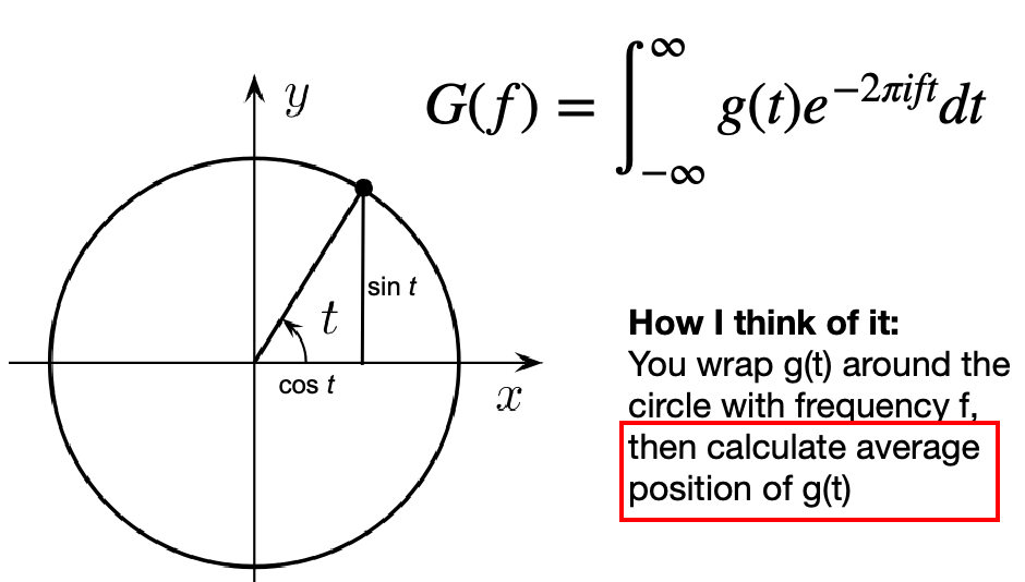
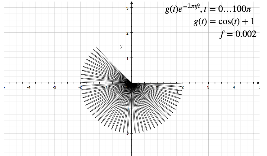
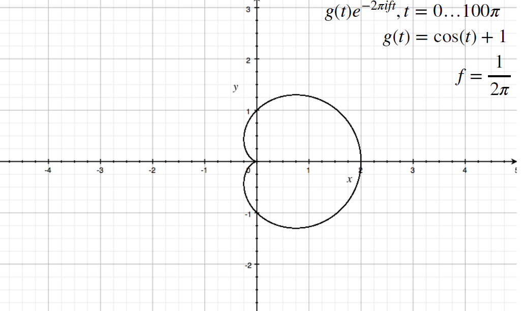
Now, consider that we are modulating the amplitude by the signal
\[g(t) e^{-2\pi ift}\]then essentially:
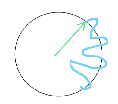
- while you are revolving the circle, you are “wrapping the original wave/signal $g(t)$” around it
Then, fourier transform does:
\[G(f) = \int_{\infty}^{\infty}g(t)e^{-2\pi i ft}dt\]which is basically can be thought as calculating the average position of $g(t)$, when given some frequency $f$
notice that:
- the function output is in frequency domain, where as the original signal is in $t$ domain
- with different frequency, the final shape/average position might be different (see below)
For Example
Consider the following original signal:
Then:
| Low Frequency | Slightly Higher Frequenct | |
|---|---|---|
 |
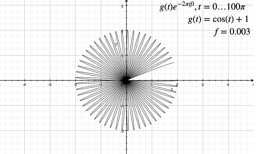 |
 |
where we notice that we only plotted for a finite amount of time, instead of $t \in [-\infty, \infty]$
-
since $g(t)=\cos(t)+1$, there are time when amplitude $g(t) \to 0$. Hence they go back to the origin on the graph.
-
for a different frequency, we have a finite amount revolved as time is finite here
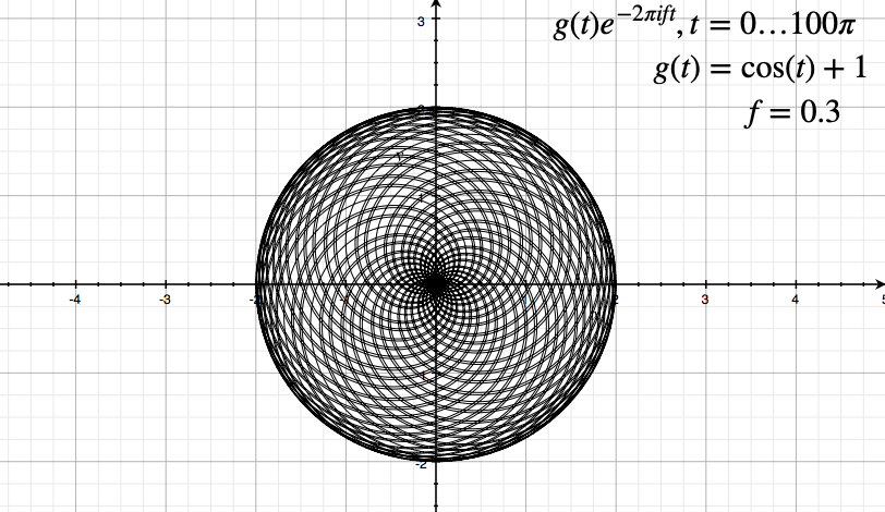
Then, if we consider the average, i.e. the center of mass, the following images
| Original | Computing $G(f)$ |
|---|---|
 |
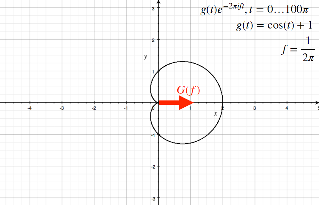 |
which then means $G[f=1 /(2\pi)]$ spits out approximately $1 + 0i$.
-
notice the output is always a Complex number.
- then, since we can do this for many different frequencies, we have a function of frequency $G(f)$
- it can be shown that the “angle” of the complex vector will always be $0$ if there is no phase.
This means that If I do a phase shift, then essentially I start the wave at another position. Hence this results in the following:
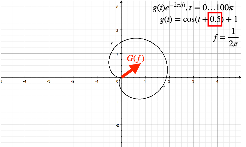
where we have rotated the circle
- so the angle of the vector has information about the phase
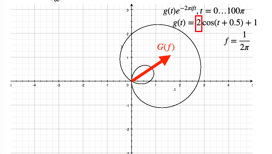
where the circle is a bit bigger.
-
so the magnitude of the vector has information about the amplitude
-
so if an amplitude of zero, this means that that frequency wave is not contributing to the $G(f)$
Then, the general formula would be:
\[G(f) = \int_{\infty}^{\infty}g(t)e^{-2\pi i ft}dt =\mathbb{R}[G(f)] + i\cdot \mathbb{I}[G(f)]\]has a real and an imaginary part, hence:
\[\begin{cases} \sqrt{\mathbb{R}[G(f)]^2 + \mathbb{I}[G(f)]^2}, & \text{amplitude}\\ \tan^{-1}(\mathbb{I}[G(f)] / \mathbb{R}[G(f)]), & \text{phase} \end{cases}\]so a single complex number output of $G(f)$ has all the information about amplitude and phase!
Note
In reality, you will have $g(t)$ taking a discrete domain (as you will see, essentially $g(x)\to g(x)$ if we think about position in the image). The number of frequencies you need to describe it will be the same as the number “positions” you have in your discrete $g(t)$, i.e. size of the domain.
Finally, for the 1D case:
Then for a higher dimension, you will just be having multiple integrals over $dt_x dt_y$ for instance:
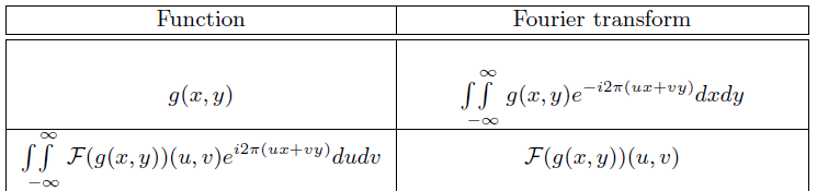
where:
- $(x,y)$ would be the position in your image, and $u,v$ would be horizontal and vertical frequencies
For Example
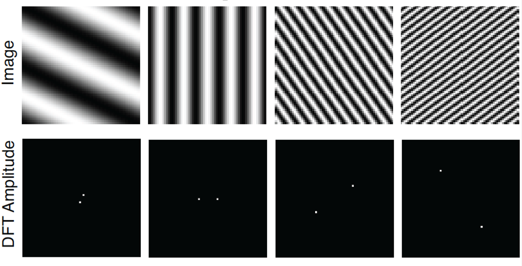
where this means:
- for the first column: the only waves that are “contributing” are the low frequency waves (because only those have non-zero amplitude/white dots). There is a tilt because the original wave in the image $g(x,y)$ has a phase.
- the higher the frequency in the image, we therefore have a larger magnitude of the vector of $G(f)$, hence farther away the activated points in the frequency domain
Note
For any signals that takes only takes real component, the amplitude will be symmetrical.
- an easy way to think about is that you will need to “cancel out” the imaginary component, as images are real
Another real life example would be:
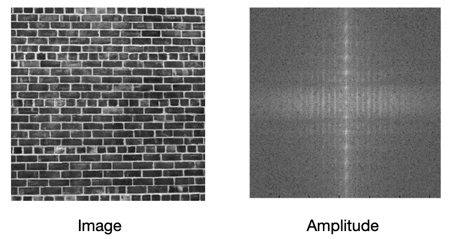
where:
- recall that horizontal and vertical component of the amplitude graph are frequencies
- in the image, horizontal sinusoids will have a low frequency component being more dominant, because the horizontal part of the image have rather slow “changes”. Hence, we have mostly low horizonal frequency activated in the $G(f)$
- in the image, vertical sinusoids will need high frequency component, since the change/sinusoids in the original image vertically is fast. Therefore, we see high vertical frequency activated in the $G(f)$
In code, this is how it is done:
cat_fft = np.fft.fftshift(np.fft.fft2(cat))
dog_fft = np.fft.fftshift(np.fft.fft2(dog))

# Visualize the magnitude and phase of cat_fft. This is a complex number, so we visualize
# the magnitude and angle of the complex number.
# Curious fact: most of the information for natural images is stored in the phase (angle).
f, axarr = plt.subplots(1,2)
axarr[0].imshow(np.log(np.abs(cat_fft)), cmap='gray')
axarr[1].imshow(np.angle(cat_fft), cmap='gray')
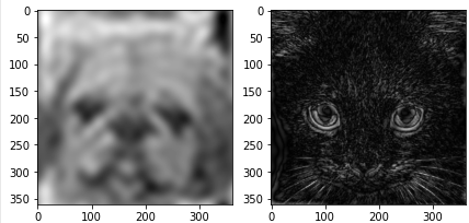
For Example: Blurring and Edge detection
Originally, we would have the image as:
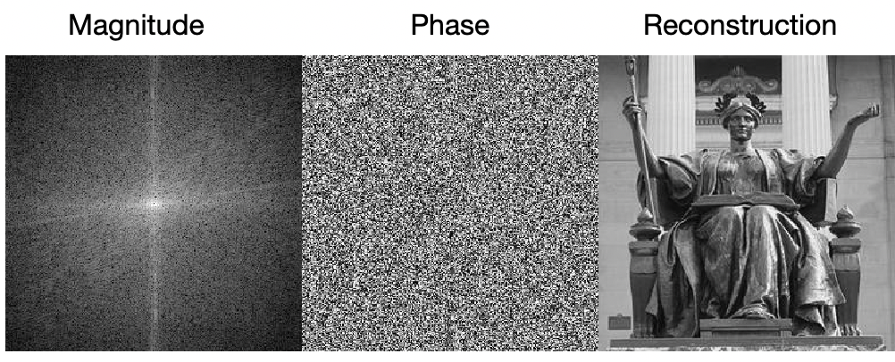
Then if we remove the high frequency
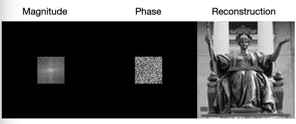
notice that:
- this is the same effect as blurring the photo (we see why convolving with Gaussian filter is the same as this soon)
Then, if we remove low frequency
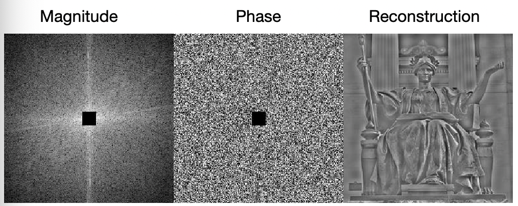
note that:
- this is the same as edge detection
In code, this is how it is done:
# we can create a low mask utlizing outer product
filter = np.zeros_like(cat_fft)
w, h = filter.shape
box_width = 10
filter[w//2-box_width:w//2+box_width+1, h//2-box_width:h//2+box_width+1] = 1

# high and low mask filter
high_mask = 1 - filter
low_mask = filter
Then applying the filter to FFT version of the image
# filtering fft, elementwise dot
cat_fft_filtered = high_mask * cat_fft # cat_fft = np.fft.fftshift(np.fft.fft2(cat))
dog_fft_filtered = low_mask * dog_fft

cat_filtered = np.abs(np.fft.ifft2(np.fft.ifftshift(cat_fft_filtered))) # shift back and then transform
dog_filtered = np.abs(np.fft.ifft2(np.fft.ifftshift(dog_fft_filtered)))

f, axarr = plt.subplots(1,2)
axarr[0].imshow(dog_filtered, cmap='gray')
axarr[1].imshow(cat_filtered, cmap='gray')
Convolution with FT
Now it turns out that:
Theorem
Convolution in $x,y$ space is element-wise multiplication in frequency space
\[g(x) * h(x) = \mathcal{F}^{-1}[\mathcal{F}[g(x)] \cdot \mathcal{F}[h(x)]]\]and convolution in frequency space is the same as element-wise multiplication in $x,y$ space:
\[\mathcal{F}[g(x)] * \mathcal{F}[h(x)] = \mathcal{F}[g(x) \cdot h(x)]\]where the 2D version of this is analogous.
This means you could speed up convolution operation since element-wise multiplication can be done fast (technically this also depends on the speed you Fourier transforms)
- if your filter is huge, then doing Fourier Transformation and element-wise dot product is fast
- e.g. if your image is size $n \times m$, and filter size $n \times m$, with padding, you will get $O(n^2m^2)$ if doing convolution
- if your filter is small, then convolution in space would be faster
- as Fourier transform takes time
- This is also why we mentioned to treat essentially an image/filter as a function! (i.e. $g(x), h(x)$ shown in the text)
For instance:
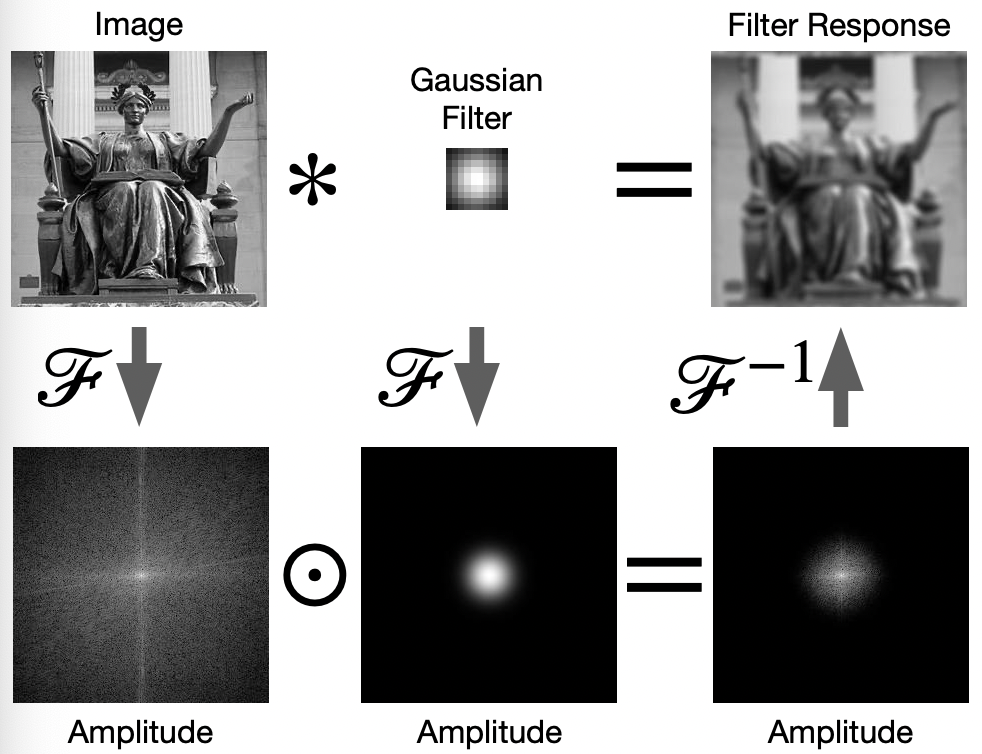
notice that:
-
in reality, applying Fourier Transform returns your a matrix of complex numbers (i.e. the vector of $G(f)$). So technically you are doing element-wise multiplication for those complex numbers
-
but for visualization, let us only consider the amplitude of the returned complex vectors in $G(f)$. (so if that is zero, than means the particular frequency wave is not useful) Then, element-wise multiplication with a Gaussian filter is basically removing high frequency details.
- note that FT of Gaussian is still a Gaussian
For Example
Now, it makes sense that why box filters have the following effect
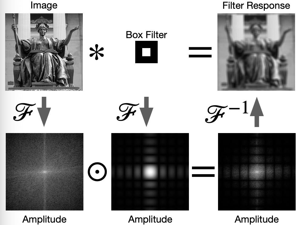
which is suboptimal as compared to Gaussian filter. This is because when we do Fourier transform for box wave:
we had high frequency terms involved!
Therefore, the FT of box filter looks like:
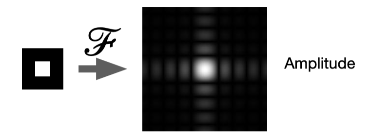
which included some high frequency noises.
For Example: Laplacian Filter
In reality, we often use the following instead of $[-1,2,1]^T$ as Laplacian filter:
This is because, if we consider the Fourier transform
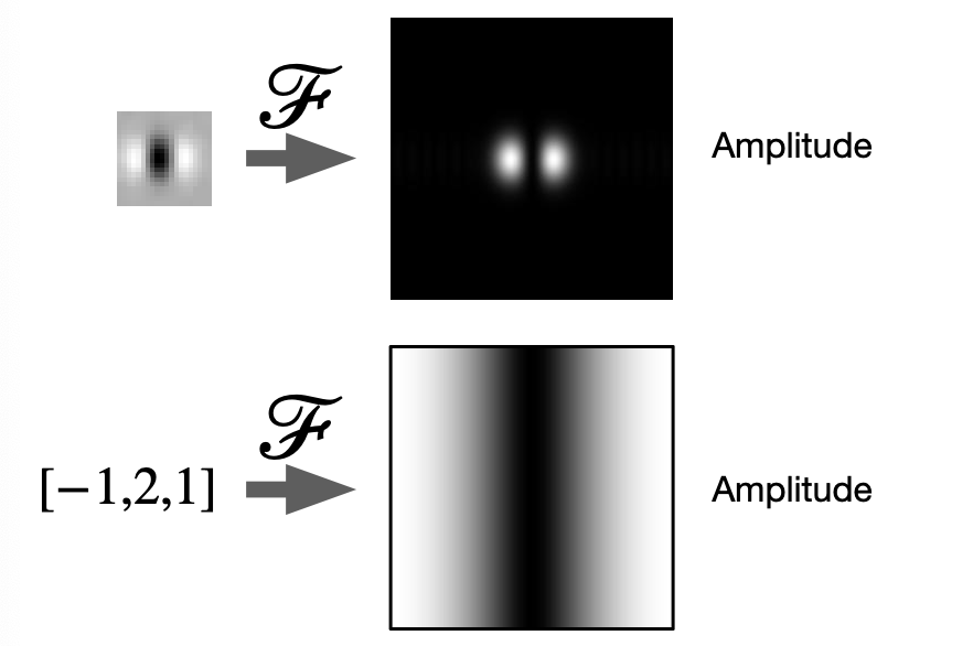
where we notice that
-
just using $[-1,2,1]^T$ would have included lots of high frequency noise, as shown on the bottom
-
but we want to remove both details and those noise to leave edges. Hence:
- involve a Gaussian blurring = removing high frequency
- perform $[-1,2,1]^T$ filter to remove low frequency details
The end product is what we see on the top, which is the commonly used Laplacian filter
Hybrid Image
This is more of a interesting application of Fourier transform. Consider the question: What frequency waves can we see from a monitor if you are exactly 150cm away?
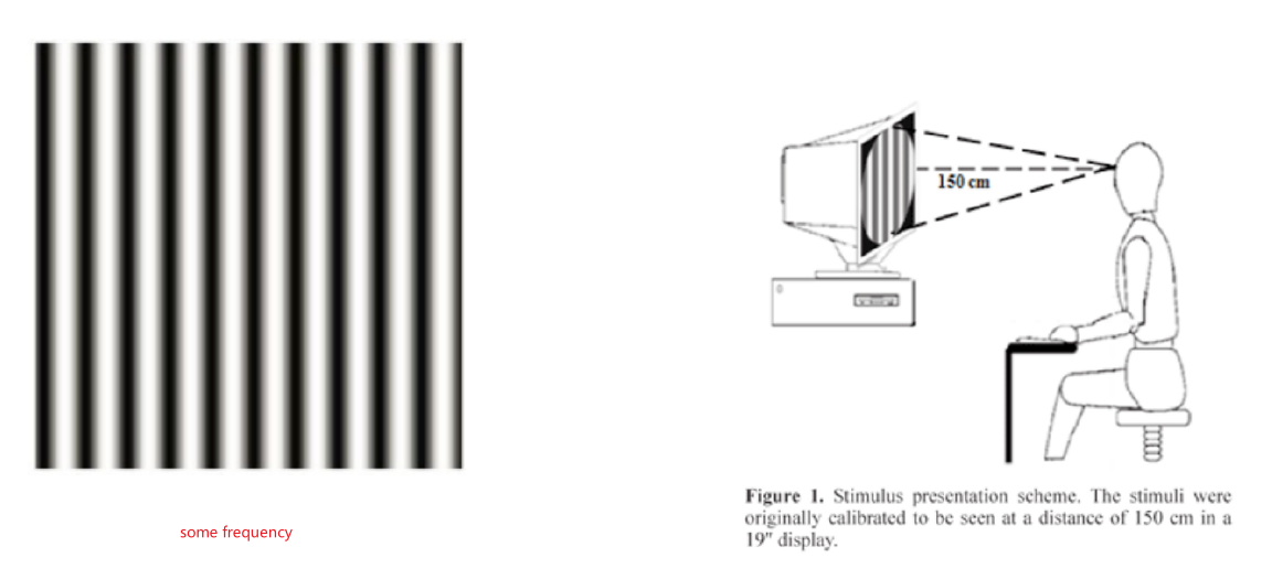
where the key idea is that you will not be able to perceive certain frequencies well.
The result shows that:
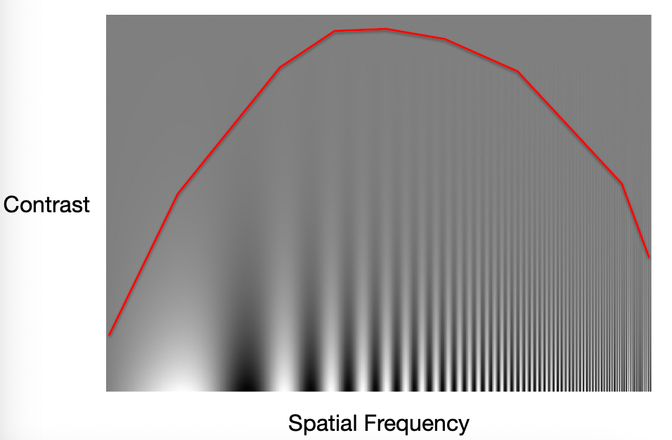
hence, any wave with configuration above the red line, people cannot see the wave/they see just grey stuff
-
contrast is brightness/amplitude
-
then maybe you can hide data above the red line
For example:
Consider keeping only low frequency data of a man’s face with high frequency data of a women’s face:
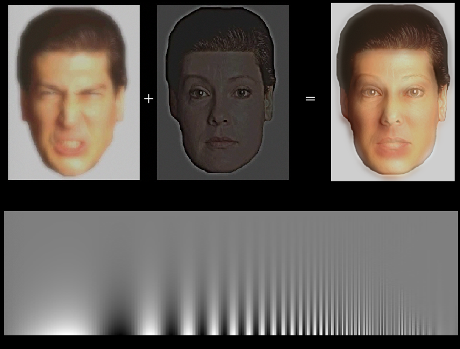
so that:
- depend on how far away you are, the red line is at different position.
- when you are far, the high frequency details you will not be able to discern. But when you are close, you will be able to see the high frequency
Then another example:
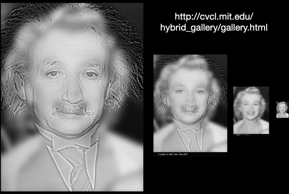
where Einstein will be encoded in the high frequency data.
- here we scaled them so you can experience see the image “from afar”
Machine Learning
If you take this class 10 years ago, you would be majorly doing maths to design filters, such that properties such as shift invariance is satified. However, it turns out that those filters/kernels can be learnt by ML/DL architectures.
- specifty the constraints, such as Toeplitz matrix, then let the machine learn it
Regression Review
Checkout the ML notes on reviewing the basics of regression
\[\hat{y}=f(x;\theta)\]where:
- $\theta$ willl be our parameters to learn
- the difference between regression/classification is basically the loss you are trying to assign
Objective function is essentially what drives the algorithm to update the parameters:
\[\min \mathcal{L}(\hat{y},y)\]Some notes you should read on:
- Linear Regression and Logistic Regression
- checkout how to prove that XOR problem is not solvable by linear models
- Convolutional Neural Network
- Backpropagation
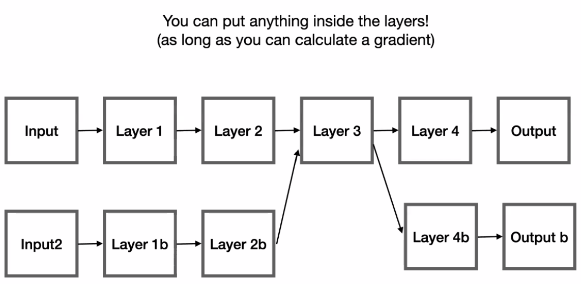
Some key take-aways:
-
Essentially we are having computation graphs
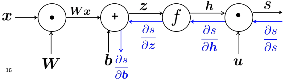
then your network architecture eventually is about what operation you want for each block.
Then, essentially you will have a loss that is a nested function:
\[\mathcal{L} = f(W^3f(W^2f(W^1x)))\]then I ask you to compute $\partial L / \partial W^1$? You realize that computing this needs:
- $\partial L / \partial W^3$
- $\partial L / \partial W^2$
Hence you realize that you can
- compute everything in one go by backpropagation.
- you have a dependency tree, where the latest layer $\partial L / \partial W^3$ will get used by all other children nodes. So it makes sense to do backpropagation.
Note:
A good trick you can use to compute derivative would be the following. Consider:
\[y = W^{(2)}h+b^{(2)}\\ L = \frac{1}{2}||y-t||^2\]And we need $dL/dh$:
-
consider scalar derivatives:
\[\frac{dL}{dh} = \frac{dL}{dy}\frac{dy}{dh} = \frac{dL}{dy}W^{(2)}\] -
Convert this to vector and check dimension:
\[\frac{dL}{dh} \to \nabla_h L\]hence:
\[\nabla_hL = (\nabla_y L) W^{(2)},\quad \mathbb{R}^{|h| \times 1}=\mathbb{R}^{|y| \times 1}\times \mathbb{R}^{|y| \times h}\] -
Correct the dimension to:
\[\mathbb{R}^{|h| \times 1}=\mathbb{R}^{h \times|y|}\times \mathbb{R}^{|y| \times 1}\]which means:
\[\nabla_h L = W^{(2)^T}(\nabla_y L)\]
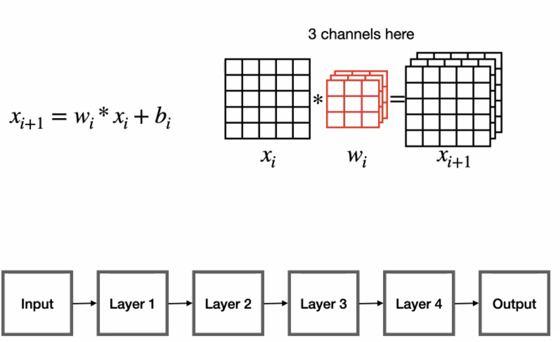
Convolution Layer Review
Review the CNN chapter of DL
-
Instead of linear layers that does $W^Tx + b$, consider doing convolution operation $*$:
Separated Compact Overview 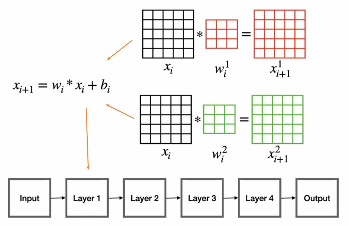
then question is then, what is the gradient of this operation?
-
another frequently used layer is max-pooling. For instance, $2 \times 2$ with stride $2$ does:
why would you want to do this?
- e.g. when you are detecting cats in an image, and certain neurons get triggered, you can use max pooling to only focus on those activated values (easier for classification head as you ignore low value ones)
- cheap resize operation which can cut down the number of neurons/connections for further layers
- the gradient defined here would be:
- $1$ for the pixel that is the max
- $0$ otherwise.
-
batch normalization also very important
\[x_{i+1} = a_i \frac{x_i - \mathbb{E}[x_i]}{\text{Var}(x_i)} + b_i\]where:
- $a_i$, $b_i$ is the scaling and shift parameter
- this is called batch normalization as this operation will be applied the same way to the entire batch.
-
dropout: a layer where with some probability we output $0$
\[x_{i+1}^j = \begin{cases} x_{i+1}^j & \text{with probability $p$}\\ 0 & \text{otherwise} \end{cases}\]which is pretty helpful for preventing overfitting.
-
Softmax: we are doing some kind of max, but also making sure we can compute the gradient
\[x_{i+1}^j = \frac{\exp(x_i^j)}{\sum_k \exp(x_i^k)}\]which can also be interpreted as a probability distribution
Then an example CNN looks like
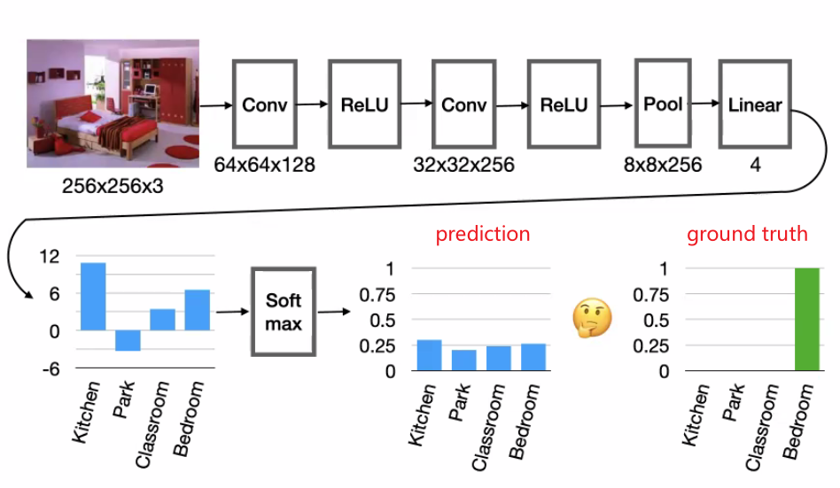
then in order to train your network/take gradient, you would need to define $\mathcal{L}$.
-
typical loss function would be cross entropy loss: Average number of bits loss/needed to encode $y$ if the coding schema from $\hat{y}$ is used instead.
\[\mathcal{L}(y,\hat{y}) = - \sum_{i} y_i \log(\hat{y}_i)\] -
once done, you can also look at the filters/weights learnt and visualize them
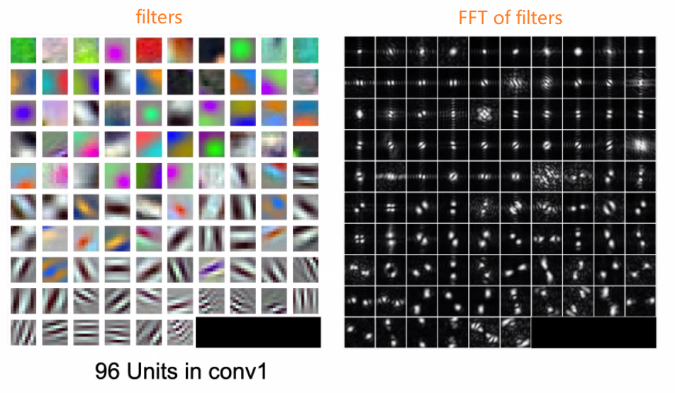
where notice that:
- the top FFT means that we are concentrating on low frequency data
- the bottom FFT shows that they look at top frequency data
Note: Why ReLU?
\[\text{ReLU}(a)=\max(0,a),\quad a = Wx+b\]Then
- One major benefit is the reduced likelihood of the gradient to vanish. This arises when $a>0$. In this regime the gradient has a constant value. In contrast, the gradient of sigmoids becomes increasingly small as the absolute value of x increases. The constant gradient of ReLUs results in faster learning.
- The other benefit of ReLUs is sparsity. Sparsity arises when a≤0a≤0. The more such units that exist in a layer the more sparse the resulting representation. Sigmoids on the other hand are always likely to generate some non-zero value resulting in dense representations.
However, there is a Dying ReLU problem - if too many activations get below zero then most of the units(neurons) in network with ReLU will simply output zero, in other words, die and thereby prohibiting learning.
Width vs Depth
We consider:
- width = how many neurons? (i.e. size of weight matrix $W$)
- depth = how many layers? (i.e. how many of those weights to learn)
In reality, there is a interesting theoretical result which is rarely used in reality
Universal approximation theorem: With sufficiently wide network and just one (hidden) layer, you can approximate any continuous function with arbitrary approximation error.
The problem is that
-
it doesn’t specify “how wide we need”, which could be extremely wide hence not computational efficient.
-
but if we go deep, we can backprop and it is in general quite fast
Object Recognition
Why is it so hard for a machine to do object recognitions?
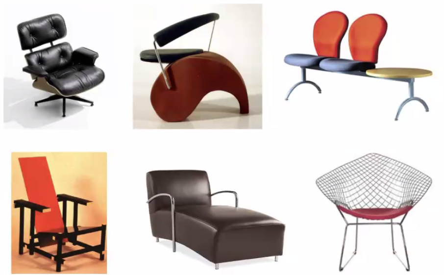
Canonical Perspective: the best and most easily recognized view of an object
- e.g. a perspective so that you can recognize this object very fast
An example would be:
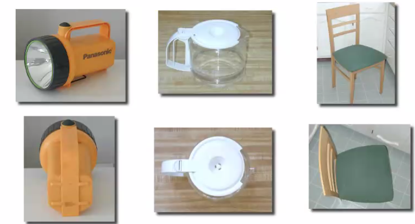
where you should feel that the top row is easier to recognize
-
how can you train a network that works regardless of the perspective?
-
model will also learn the bias
e.g. all handles are almost all on the right!
Entry Level Categories: The first category a human pick when classifying an object, among potentially a tree of categories that corresponds to an object.
An example would be:
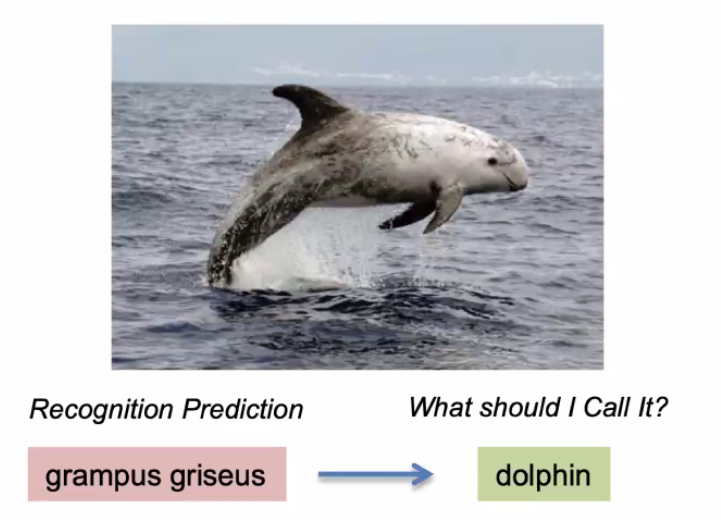
the question is, why did you think of this as a dolphin, but not saying it is “an animal”? A “living being”?
Other problems involve:
- scale problem
-
illumination problem
-
within-class variation
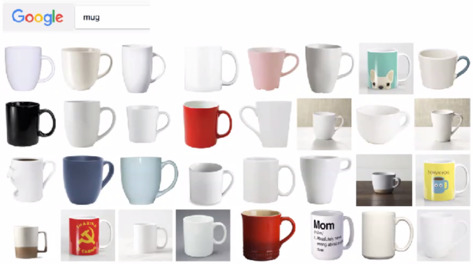
Note
- In reality, many massive models are trained with data coming from crowdsourcing: paying people around the world to label data (e.g. Amazon Mechanical Turk)
- one large image dataset commonly used is ImageNet - often used as a benchmark for testing your model performance.
Classical View of Categories
One big problem is “what is xxx”? Hot Dog or a Sandwich?
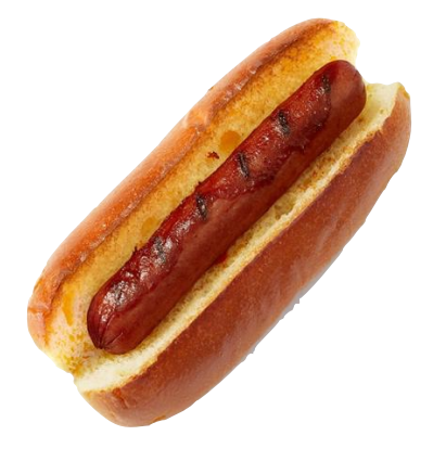
Some natural ways a human think about categorizing an object:
- A category is formed by defining properties
- Anything that matches all/enough of the properties is part of the category
- Anything else is outside of the category
But even this idea could vary, in different people/culture.
-
e.g. in some indigenous people in Australia, people have a single word for “Women, Fire, and Dangerous Things”
-
e.g. in a culture, what are the words you use to represent colors?
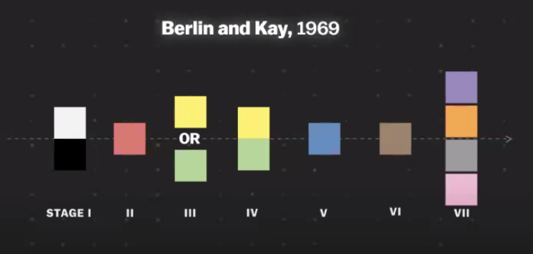
where:
- if you only have two words for color, which colors will you pick? Black and White
- for three colors, most people gives Red
- the take-away message is that you can think of things even if you don’t have language for it. Yet for machine models, we are categorizing objects based on language (i.e. language label for category)
Another way to define category would be:
Affordance: An object is defined by what action it affords
- e.g. what we can do with it
- e.g. a laptop is a laptop for us, but could be a chair for a pet
A theory of him is that when we see an object, we automatically think about affordance of it, i.e. what we can do with it.
Two Extremes of Vision
In reality, we are always dealing with either of the two occasions:
- we don’t have much data, we need extrapolation to predict things
- we have much data, we need to interpolate and find differences between existing objects
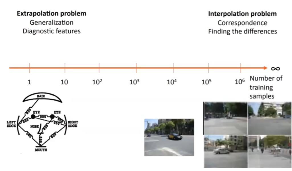
where:
- the latter end of the spectrum would be captured more by NN types of model, which tends to be poor at generalization, so we care a lot of few-shot training/zero-shot training
- for huge training dataset, one reason for test accuracy to be high is that the training dataset distribution does model the true distribution, hence “overfitting” will not really damage performance.
Exemplar SVM
In reality approaches that uses big data to do basically lookup function for classification.
One example is the Exemplar-SVM
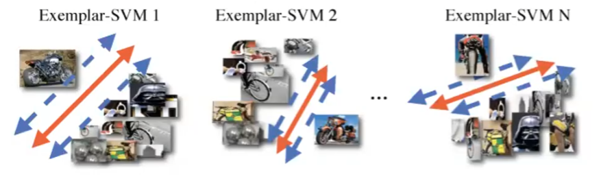
this idea can be seen as a new way to do classification. For example data in the training set, train a SVM where that single data point is a positive example, whereas all the others are negative. Graphically:
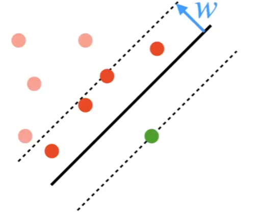
Therefore, you learn $N$ SVM, if there are $N$ data points. With this, when you are classifying an input $x$, all you need to do is to ask is: to which of the $N$ data point is it most similar to w.r.t the SVM? (hence it is like a k-NN). Then, when giving an image, you do:
- for each possible window in an image
- try all the $N$-SVM and pick out the SVM that fires the most (hence it is like a lookup table)
- Since each SVM trained corresponds to an object, this can be used for object recognition
Graphically
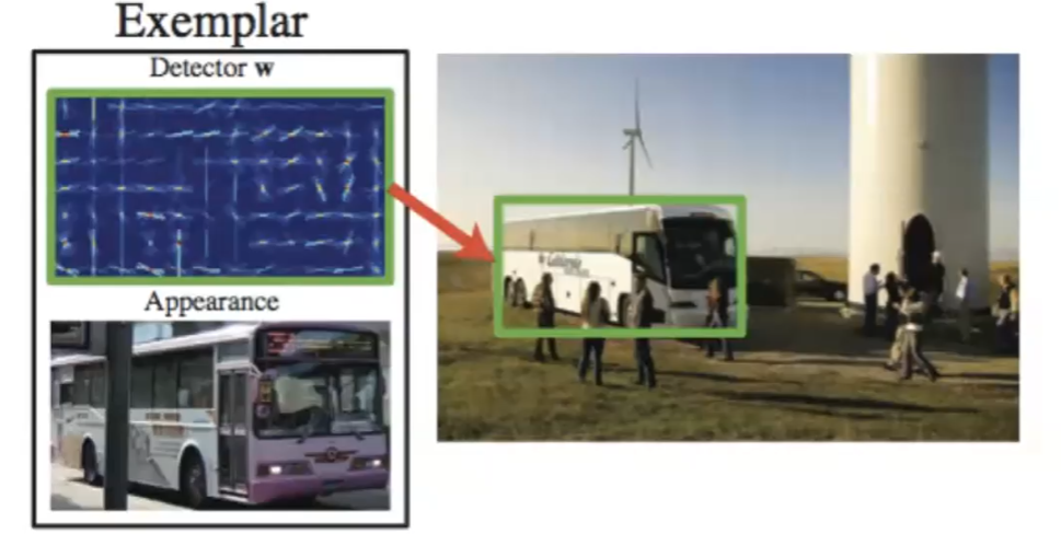
where notice that:
- since SVM gives some degree of extrapolation/robustness, it works even if the bus has a different color.
This works essentially based on the idea that, instead of definition what is a car, we consider what is this object similar to (something we already know)?
This setup in the end can also do segmentation and occlusion, just because there are many repetitions in our real world.
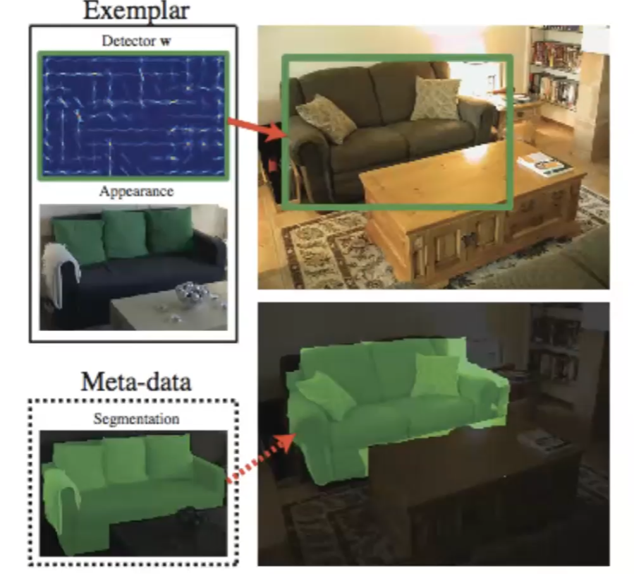
where the above would be an example of segmentation
What might not work:
- there is a view-point bias for photos, so that technically if you change the view point, the SVM might not work. However, again, assuming we have huge data, there could be essentially many images taken from many viewpoints. Then it still works.
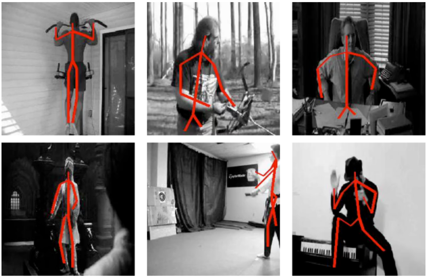
Deformable Part Models
This idea is then to learn each component of the objects + learn the connections. This would work extremely well at detecting poses, for instance, where all we changed is the connection between components of the object (human).
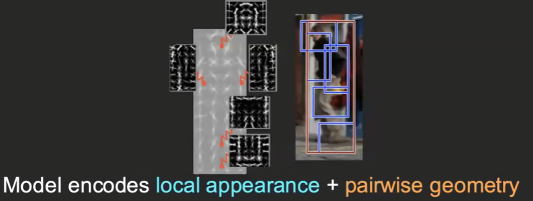
Specifically, you would build a tree that connects the
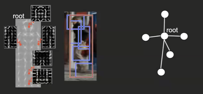
where:
- nodes encode the component we recognized, e.g. the
rootwould be the torso, and etc. - edges encode the relationship we found, e.g. relative relationship between leg and torso.
Therefore, as it can recognize individual parts + connections, it can work with different view points.
Specifically, this model does the following as the objective for similarity:
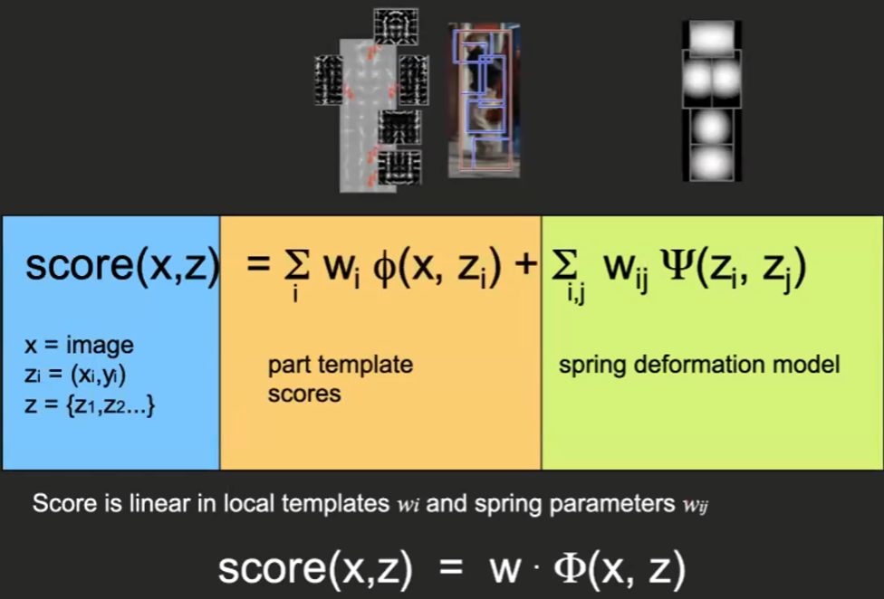
where:
-
$z_i$ is the location of the different parts/components
-
part template refers the score for the position nodes w.r.t the large image
-
deformation model refers to the score for the edges w.r.t the pair of node, e.g. answering the question: what is the score if a leg is below a torso?
R-CNN
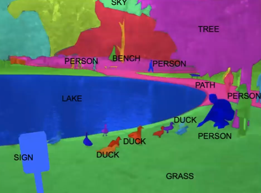
Consider a task that tries to assign a category to each pixel:
The idea is basically to:
- consider all possible windows (of various sizes) in an image
- for each window:
- in each of the window, classify if we should continue processing it
- if yes, put it into CNN and classify the window
Graphically, we are doing
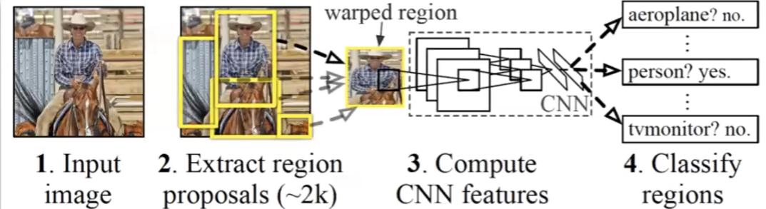
and it works pretty well in reality. However, the problem is that it is slow. Therefore we also had models such as Faster CNN, by learning the window proposition step, i.e. which windows are plausible, hence reduce the time.
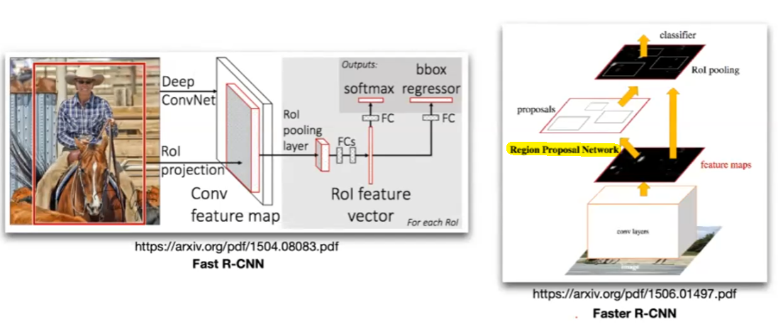
then you basically just backpropagate to update the weights:
- initially the convolutional layer at the bottom of right image would consider all possible windows
- the Region of Interest feature vector would encode the proposed window, then you compute loss to the window proposed as you know the bounding box
- in faster RNN, the feature maps are used two fold: used for proposal and being passed on as encoding what is inside the window
Segmentation Examples
Consider the task to assign each pixel of the image a label: either a category, or whether if it is a new instance. This task is commonly referred to as segmentation.
Some architecture that aims to solve this include Fully Convolutional Network
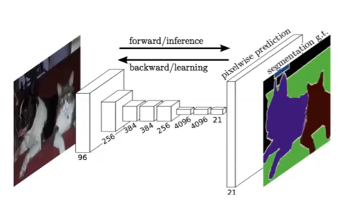
Essentially you can just keep doing convolution, so the output is still an image
Encoder-Decoder type.
Here the idea is that, in order to be able to recognize a “bed”, you need to somehow encode all the related pixels into a group and recognize this group of pixels is a bed.
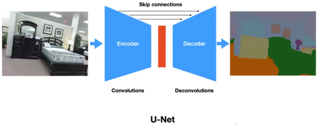
where essentially the latent feature space would be able to encode/compress pixels. However, this does mean resolution loss in the output image, hence we also have skip confections added.
Residual Networks
The observation comes from the abnormal behavior that, increasing the layers actually caused a decrease in performance for both train and test:
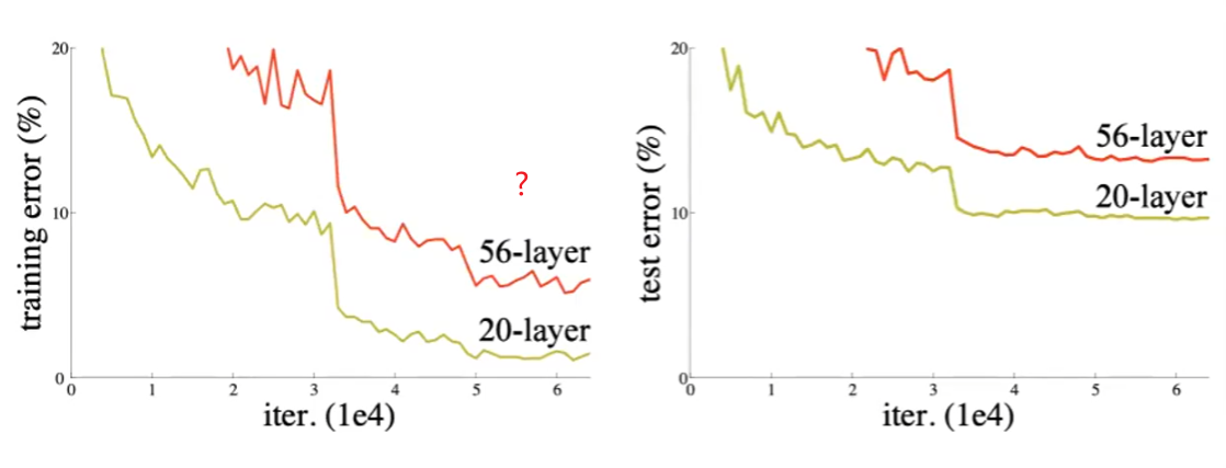
this is abnormal because, if the 20-layer solution is optimal, then the other 36-layers should be able to learn to do nothing, or doing identity operation.
Then, the intuition is to make learning nothing an easy thing to do for the network. Hence:
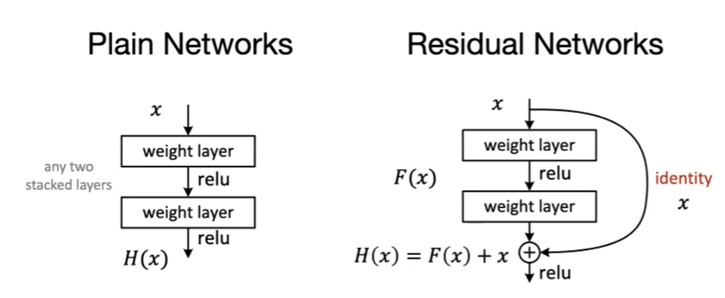
where essentially we can have $F(x)=0$ being pretty easy to do (v.s. $F(x)=x$ with nonlinear operation is pretty hard).
- This is also helpful for solving vanishing gradient
- essentially enabled us to train very deep networks!
Again, the key reason behind all the idea of training deeper network is that you have big data for training.
Video Recognition
Theory of mind refers to the capacity to understand other people by ascribing mental states to them. In terms of CS, it is like you have the same program, but different memory. Yet you still can more of less know what the program will do.
First of all, we need to represent video as some kind of numbers. Consider videos as a series of pictures:
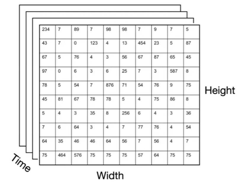
Then essentially you just have a cube of pictures/matrix.
Accordingly, convolution operation thus involve a third dimension
| 2D Convolution | 3D Convolution |
|---|---|
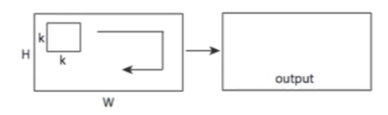 |
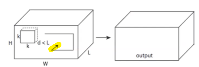 |
where now essentially you have an increased dimension in kernel + another dimension of time for the kernel to move around (convolution).
-
first imagine the video as a grey scale image, then essentially from image convolution (2D kernel) we now have video convolution (3D kernel)
-
note that because the filters basically also have a time dimension (stacks of 2D kernel), so they can be represented as a video as well.
Human Behaviors
Before we consider how machines should solve the problem, we should first understand and look around how human solve those problems such as:
- action classification: what is he doing (given a video)? Is his action intentional/unintentional?
- action prediction: what will happen next?
Behavior Continuum
Consider the case when a children goes to school, an continuous set of events that he/she would do involve:
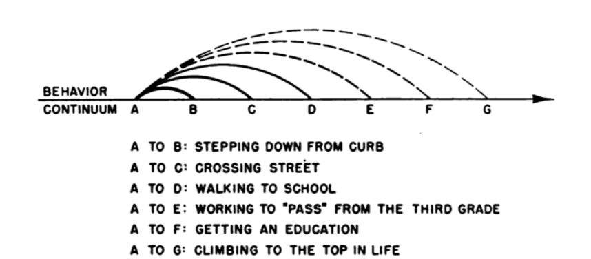
for example, doing $A-G$ would have included doing $A-B$, etc.
- this poses the question of how to quantitatively represent an action hard, as it’s no longer discrete
- this then relates to how we perhaps want to design video recognition
Human Brain Video Recognition
Essentially a video is a stack of images, such that if flipped through fast enough, we have the illusion that things are moving. How does a human brain understand videos?
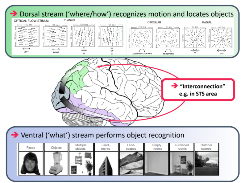
where essentially:
-
we are doing two separate systems: one that performs object recognition and the other recognizes motion/location.
-
an example would be the stepping feet illusion: our dorsal stream regonizes dots moving around as a person walking
Therefore, one idea is to build a network also with two visual passways:
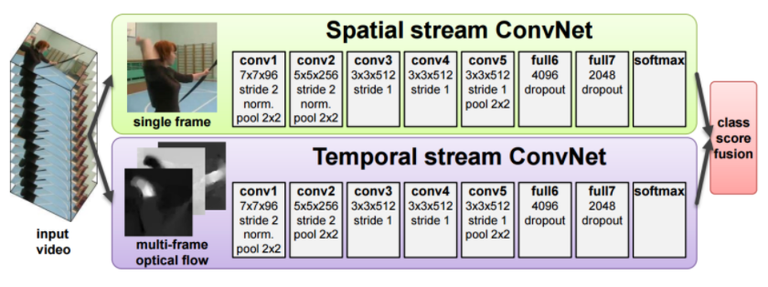
where:
- the spatial stream is basically the normal convolutional net
- the temporal stream basically is the convolutional net but the input is optical flows, how each pixel in an image moves
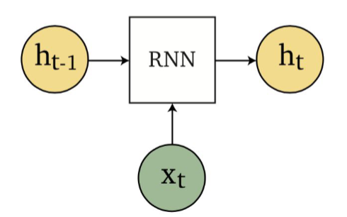
Recurrent Neural Network
Another way to represent time would be naturally the recurrent neural networks. When unrolled, basically does:
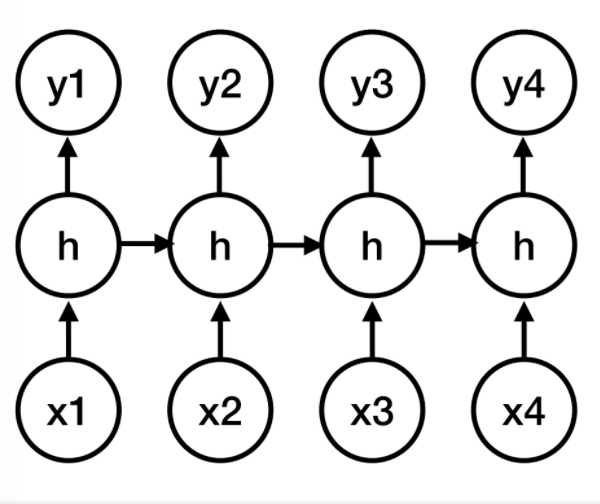
where the “forward” formulas becomes:
\[h_i = f(w_x^T x_i + w_h^t h_{i-1})\\ y_i = g(w_y^T h_i)\]where interestingly:
-
with the additional of time, another way to see this is that we now can do loops in FFNN.
-
basically now we have a state machine:
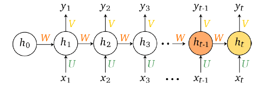
Though this network is sound, the problem is that it has a problem of vanishing/exploding gradient. Because when you backpropagation, you would be doing backpropagation through time: (TODO replace $z_i$ with $h_i$)
At time $i$, we have the forward pass being
\[z_i = h_i = f(w_x^T x_i + w_h^T h_{i-1})\]then the gradient being:
\[\frac{d\mathcal{L}(\hat{y} , y)}{dw} =\frac{d\mathcal{L}}{dz_{i+1}} \frac{dz_{i+1}}{dz_i}\frac{dz_{i}}{dw} = \frac{d \mathcal{L}}{dz_T}\left( \prod_{j=1}^{T-1}\frac{dz_{j+1}}{dz_j} \right)\frac{dz_i}{dw}\]being the general form.
- e.g. let $w = w_h$. (recall that only three weights). Then the update/gradient at the end of the sequence at time $T$ will be products of gradients, which would either explode or vanish if it is large or small.
- to solve those problem, we have GRU/LSTMs.
GRU and LSTM
Schematically, GRU does the following change:
| RNN Encapsulation | GRU Encapsulation |
|---|---|
 |
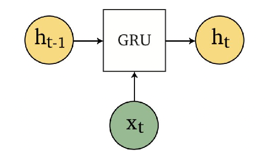 |
Specifically:
| GRU Schematic | Equations |
|---|---|
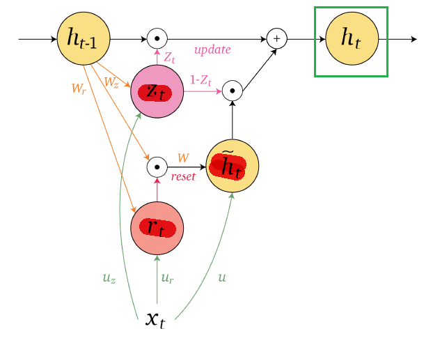 |
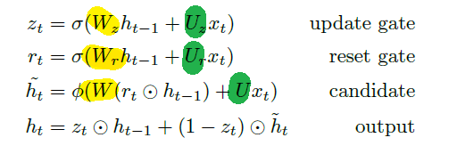 |
Similarly, the LSTM architecture looks like:
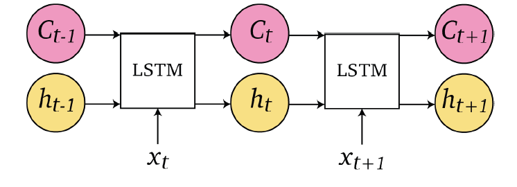
note that you have an additional memory cell, $C_{t}$, as compared to the GRU and RNN we had.
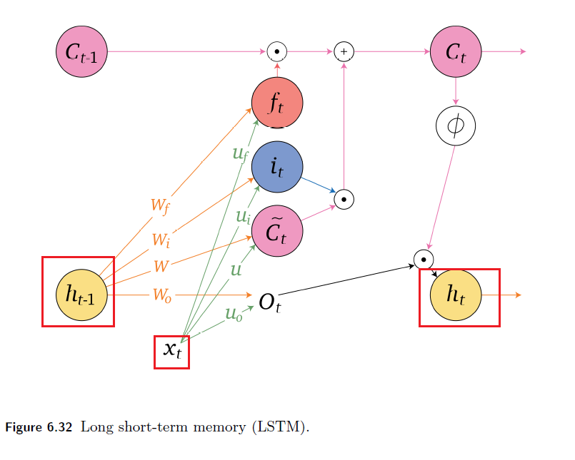
Each unit of LSTM look like:
| LSTM Schematic | Another View |
|---|---|
 |
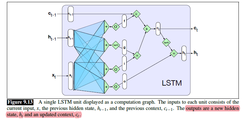 |
where the highlighted part is clear, same as RNN.
(a good blog that discuss LSTM would be: https://colah.github.io/posts/2015-08-Understanding-LSTMs/)
In both cases, the backpropagation through time would now involve addition instead of products. Hence this aims to solve the exploding/vanishing gradient problem.
Action Classification
The basic approach used here is to learn motion Features
- e.g. elapsed time feature
Key aspects of motion/video that we seem to care about:
- how long does each action take? i.e. normally, what would be the elapsed time for a normal motion.
- what are the main objects/what will happen next?
One way to learn this in NN is that we can resample a video, and then ask the NN to predict elapsed time:
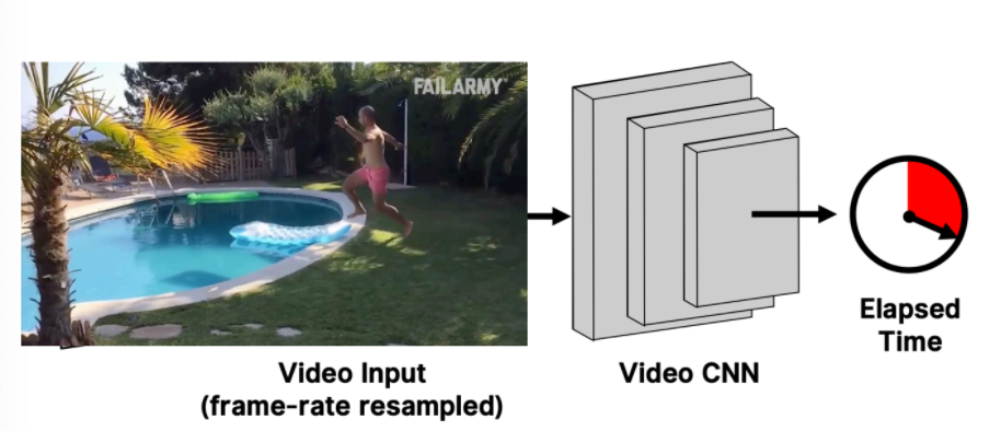
This feature can be helpful for:
- deciding whether if an action is intentional/unintentional: speed of action alters perception
Action Prediction
It turns out that all our mind cares is about the future/actions, i.e. for things that seem irrelevant in the future, we kind of just ignores it.
- correlates to the idea before that categorization of an object is related to intention/action we can do with it
An example to stress how to predict the future would be:
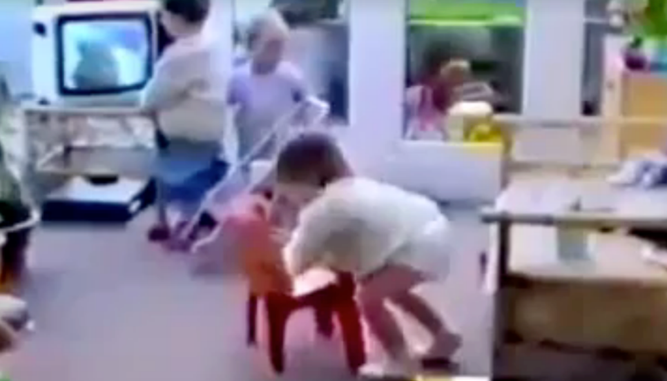
this will be called future geneation:
- given data up to $x_t$
- predict $x_{t+1}$
Then for each video you collected in your dataset:
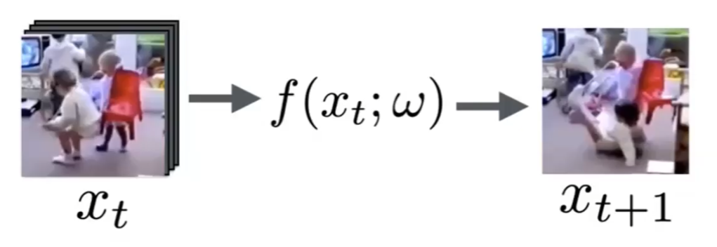
with loss being
\[\min_w \sum_i ||f(x^i_t; w) - x_{t+1}^i||_2^2\]which basically is a Euclidean loss:
- each vector $x^{i}_t$ represents the flattened vector representation of video at time $t$ (hence an image), for the $i$-th video in your dataset
But consider $x_{t+1}^i$ being the $i$-th possible future of the video up to $x_{t}$. Now you want to output, say, all possible futures, and perhaps among them, pick the most probable future.
- note that our brain can do this pretty easily!
Then, we see a problem that with this is that you can let:
\[f^*(x_t;w) = \frac{1}{m}\sum_i x^i_{t+1}\]to regress to the mean, i.e. your predicted future would be a mean of possible futures. This is bad! But how do we build models that is capable of predicting possible/likely future?
One problem is that there are multiple possible outcomes (i.e. we have uncertainties in what will happen next), but the reality we have in the video has only one future. How do we build this?
Intuition:
When a child gets near a candy store, and right before he/she goes inside, what will he/she predict to happen inside?
- instead of saying how many candies, and their color, he/she might predict his/her own sensation: they are going to taste like xxx, smell like xxx, and etc.
Therefore, the idea here is to build a NN with:
- input $x_t$, e.g. a picture
- predict the features of the future picture $x_{t+1}$. (the feature could come from an encoder that encodes $x_{t+1}$ for example)
Graphically, we are doing:
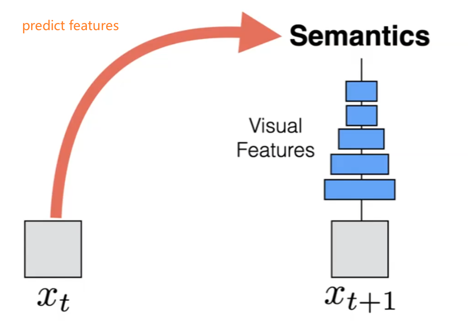
which is an easier prediction problem, because the output space is much smaller.
Then, since there are multiple possible futures, we could have each multiple predictions of the feature:
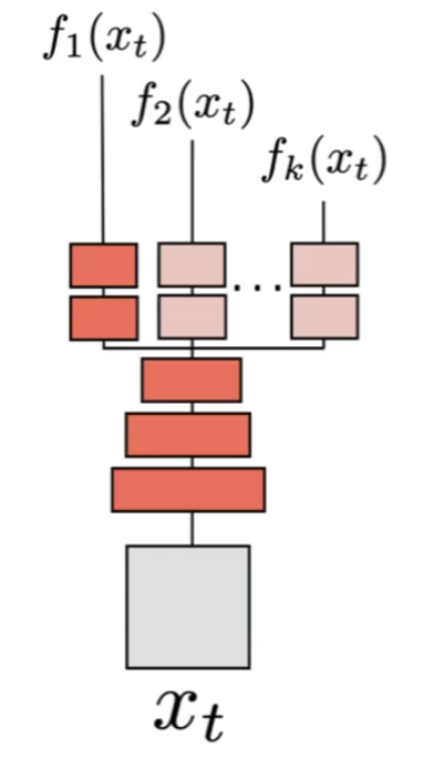
which we can do by basically having $k$-learnable activation functions/NN attached after. But then, to train this multiple prediction model, notice that we only have one output/future in the video data, hence only “labeled feature” $g(x_{t+1})$:
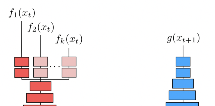
so then the problem is how to figure out the whole distribution ${f_1(x_1),f_2(x_1),…,f_k(x_1)}$ while you only have one label/ground truth $g(x_{t+1})$. Then, the idea is:
-
We know that if we only have one prediction, then we can do:
\[\min_f \sum_i ||f(x_t^i) - g(x_{t+1}^i)||_2^2\]for the $i$ data points you have in your training set.
-
If we have only one of them correct, but I do not know which one, then it means we have some latent variable to estimate.
For a single data point $x_t$, the loss would be:
\[\sum_k \delta_k ||f_k(x_t) - g(x_{t+1})|| _2^2\]for $\delta_k \in {0,1}$ being a latent variable, so that $\vert \vert \delta\vert \vert _1 =1$.
Then for all those data points, we have a different $\delta_k$ to learn:
\[\min_{f,\delta} \sum_i \sum_k^K \delta_k^i ||f_k(x^i_t) - g(x^i_{t+1})|| _2^2,\quad \text{s.t. } ||\delta^i||_1=1\]for basically $\delta^i$ being like a one-hot vector to learn.
Now we have the entire problem setup, lastly we need to train this.
- this using backprop does not work, because $\vert \vert \delta^i\vert \vert _1=1$ makes this a discrete variable, which we cannot take derivative of.
- but since it is a latent variable, use EM algorithm
- E-step: Fill in the missing variable ($\delta$) by hallucinating (if at initialization) or estimating it by MLE (when you have some $f$)
- M-step: Fit the model with known latent variable ($\delta$), and do backpropagation on $f$ to maximize the parameters for $f$.
- repeat
where essentially it solves the loop by “hallucinating”:
- to solve/optimize for $f$, we need $\delta$; but to solve/optimize for $\delta$, we need $f$.
- therefore, we just assume/hallucinate some $\delta$ to start with, then iteratively update
Examples: Then we can use this to do action prediction, with $k=3$ and predicting four features (handshake, high five, hug, kiss):
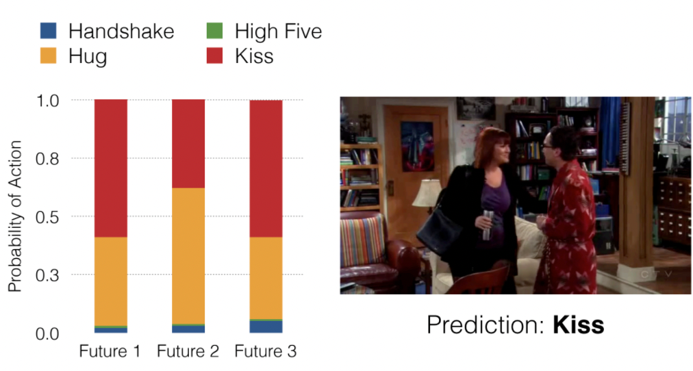
For prediction, we then use $\delta^i$ to tell which future is taking place, and then spit out the feature that has the highest score as the prediction.
Another idea is that, since someimtes we have uncertainty in actions (even if we do it by ourselves)
Predicting in Eucliean Space
Last time we saw that the objective we used results in the problem of regression to the mean:
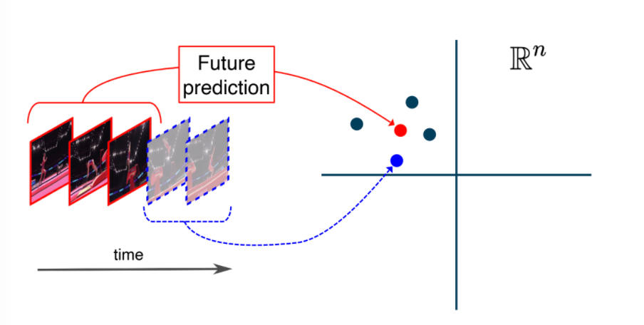
where basically
- you imagine the four possible futures, indicated by the three black points and the blue point
- the “possible futures” are obtained by having similar videos and claiming their “past” are the same even though there are some variations
- one idea of how we “fix” this is to represent this perhaps not in the input feature space
First, we need to recap what properties eucliean geometry have.
Hyperbolic Geometry
Axioms of Eucliean Geometry: (i.e. we can derive all euclidean stuff from those five axioms)
-
There is one and only one line segment between any two given points.
-
Any line segment can be extended continuously to a line.
-
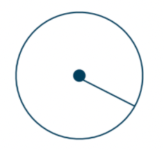
There is one and only one circle with any given center and any given radius.
-
All right angles are congruent to one another.
-
Given any straight line and a point not on it, there exists one and only one straight line which passes through that point and never intersects the first line.
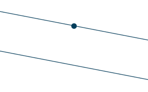
basically related to what it means being parallel.
For hyperbolic geometry, we only chage the fifth rule and we will have a different geometry:
- Given any straight line and a point not on it, there exists
one and only oneinfinitely many straight line which passes through that point and never intersects the first line.
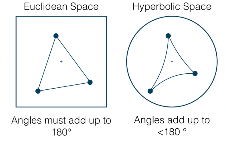
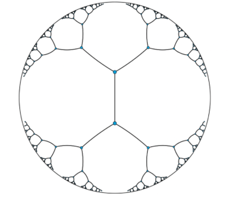
Some graphical comparision would be
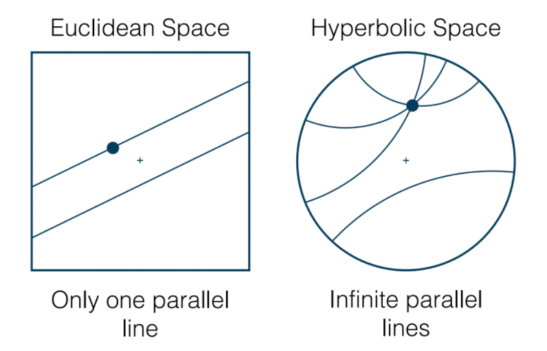
where
- the plus sign represents the origin.
- for hyperbolic space, the infinity of the space is the circular boundary
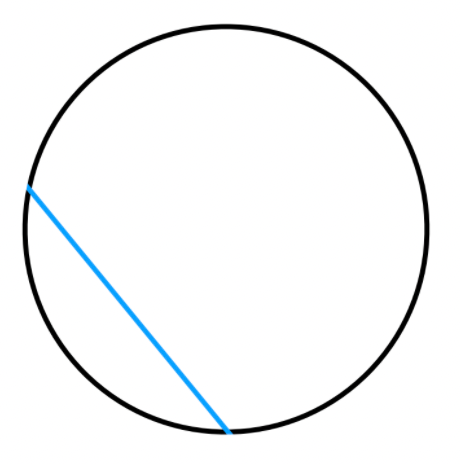
- the straight line in hyperbolic space is drawn by doing the shortest path in the manifold (see below).
- This line is also called the geodesic line, which in cartesian would be a straight line.
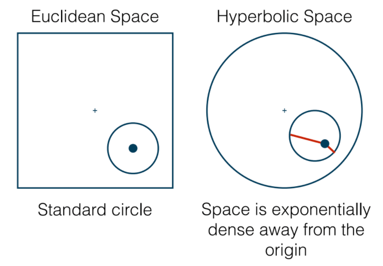
- one intition here is that the density of space is high near the boundary of the hyperbolic space.
All the points live oin a manifold, where the manifold is the hyperbolic surface in this case (the blue region above, generated by rotating a hyperbole)
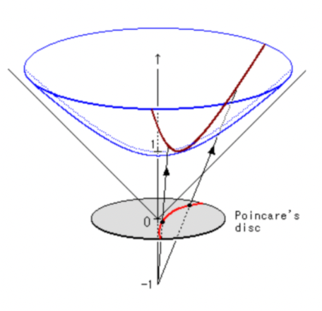
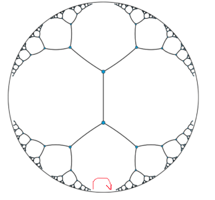
Then the formula for distance between points on hyperole (the blue surface), becomes:
\[d(a,b) = \cosh^{-1}\left( 1+ 2 \frac{||a-b||^2}{(1-||a||^2)(1-||b||^2)} \right)\]for $a,b$ being vectors to the points. Some other properties of space include:
| Shapes in Hyperbolic Space | Center of Circles |
|---|---|
 |
 |
where:
- on the left, it is significant as the area of triangle will be solely determined from angles. And the shape of “square” does not exist (though there exists four sides shapes)
- on the right, the center of circle shears more towrads the boundart, because the density is higher near boundary (i.e. the red curves, technically it sohuld be, should have the same length!)
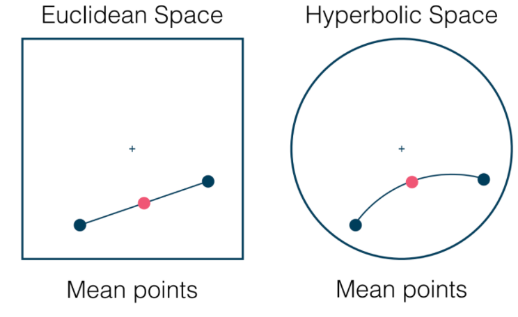
Additionally, you can also find the mean (which now relates to regression!)
Distortoin of Space
Why do we want to use eucliean space? We want to embed a hierarchy tree in to the space.
I want distance defined by a line joining the nodes should be the sum of distancce between between node-node in the tree.
Consider doing this in eucliean space, this does not work and we have distortion:
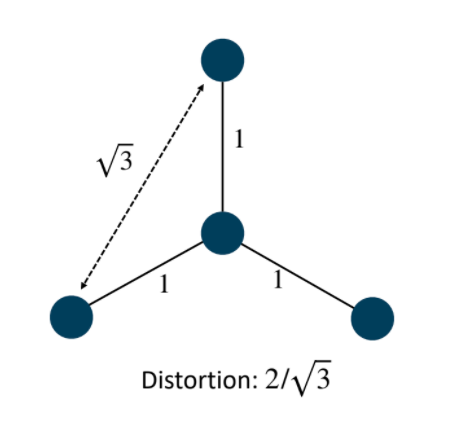
where this comes from $2=1+1$ is the correct distance we want, and $\sqrt{3}$ is the actual distance we got.
Yet, hyperbolic spaces can naturally embed trees
| Trees in Hyperbolic Space | Example | Example |
|---|---|---|
 |
 |
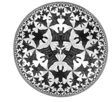 |
where the
- second figure shows an example of “straight line”/shortest path that defines the distance between the two nodes.
- third figure shows bats that have the same area in hyperbolic space
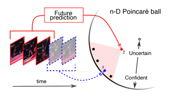
Predicting in Hyperbolic Space
Then we consider 4 possible futures, shown as the three black points and a single blue point. Our task is to predict $\hat{z}$ given the three past images, and the 4 true labels such as $f_\theta(\text{past images}) = \hat{z}$ represents the mean of the future = minimize the distance to the all the possible futures:
| Regressoin Task | Interpretation |
|---|---|
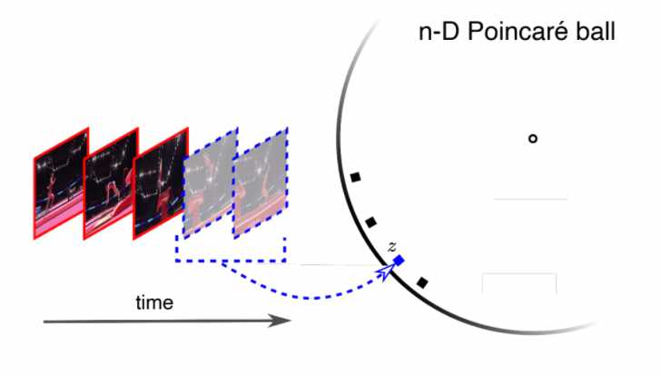 |
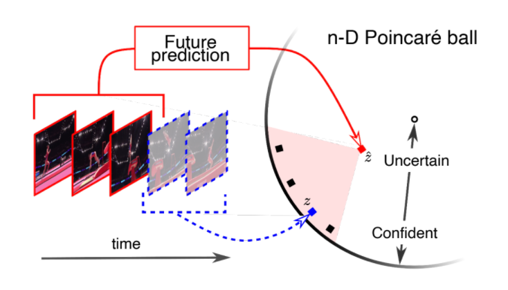 |
where:
-
regression to mean in hyperbolic space means having the point $\hat{z}$ which is closer to origin, which corresponds to uncertainty in or prediction being in higher parts in the hierarchy tree!
-
Then, the objective function would be defined by regression using hyperbolic distance
\[\min \sum_i\left[ d^2 (\hat{z}_i,z_i) + \log \sum_j \exp (-d^2 (\hat{z}_i,z_j)) \right]\]such that we essentially have two neurnets, $z_i$ from the blue neural net and the $\hat{z}_i$ from red for future prediction:
- the first term minimizes the distance between $z_i$ and $\hat{z}_i$, for $z_i$ being the one past, and $\hat{z}_i$ being its future
- technically we are predicting one $\hat{z}_i$ per past, but eventually we converge to the same future $\hat{z}$ if the past are similar
- the second term wants $\hat{z}_i$ to be far away from other non-related examples $z_j$ in the dataset (without this term $z,\hat{z}$ collapse to origin)
Graphically:
where the blue latent point can be interpreted as “what features in the future image”
- the first term minimizes the distance between $z_i$ and $\hat{z}_i$, for $z_i$ being the one past, and $\hat{z}_i$ being its future
Last but not least, given those points in the latent space, you finally map it back to features such as “probability of hugging”, and etc:
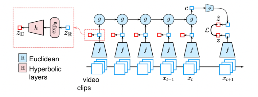
where the classifer you attached from the output of latent space vector $z$ could be a linear one in hyperbolic space.
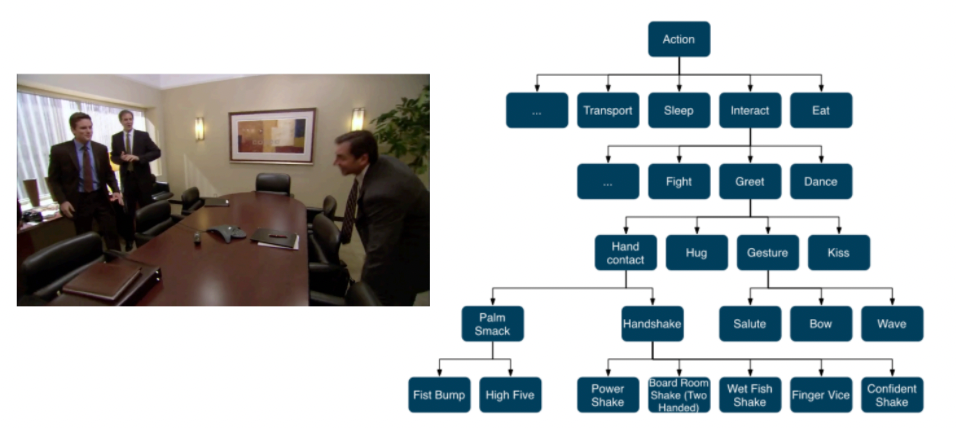
Predicing Action
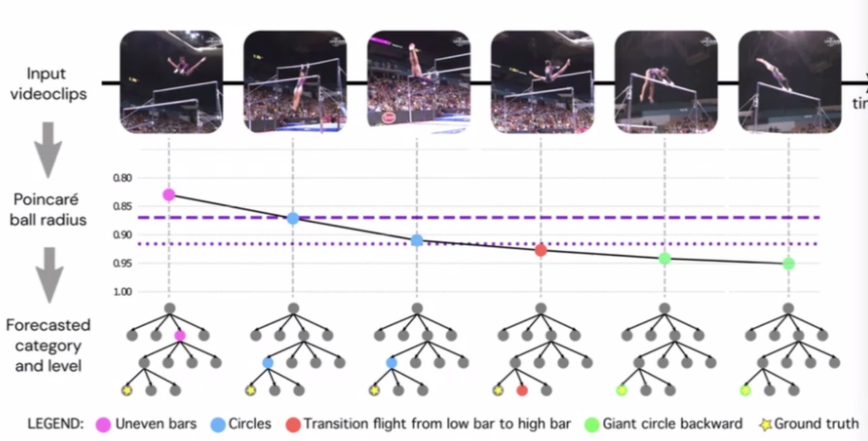
notice that:
- essentially as more future is revealed, the less uncertainty you have by moving down the action hierarchy tree
- the purple dash lines would represent the levels of the tree you are at
Action Regression
Other related applications include regression on actions to predict a score.
For example: How well are they diving?
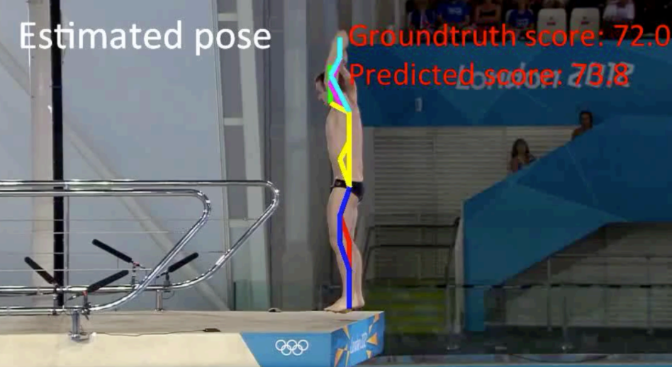
- Track and compute human pose
- Extract temporal features
- normalize pose
- convert to frequency space
- use histogram as descriptor
- Train regression model to predict expert quality score
Additionally, this can also be applied reversely by answering the question: how should the post change to get a higher score?
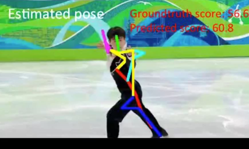
where
- essentially compute gradients
Object Tracking
The first and foremost useful representation of motion is the optical flow.
Optical flow field: assign a flow vector to each pixel
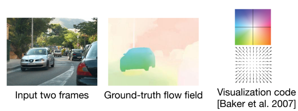
However, there is a problem with computing optical flow, e.g:
| Start | End |
|---|---|
 |
 |
which is ambiguous how the line moved, as it could have go up/right/top right, all yielding the same result.
- another example would bte the barber pole illusion, where
- e.g. if you put an aperture near the car, then how it moves become ambiguous. Hence this where machine learning becomes useful, which can learn the priors. But the problem is where can we get the correct labels if we have those ambiguities?
Learning Optic Flow
The idea is to training use game engines, so that we can:
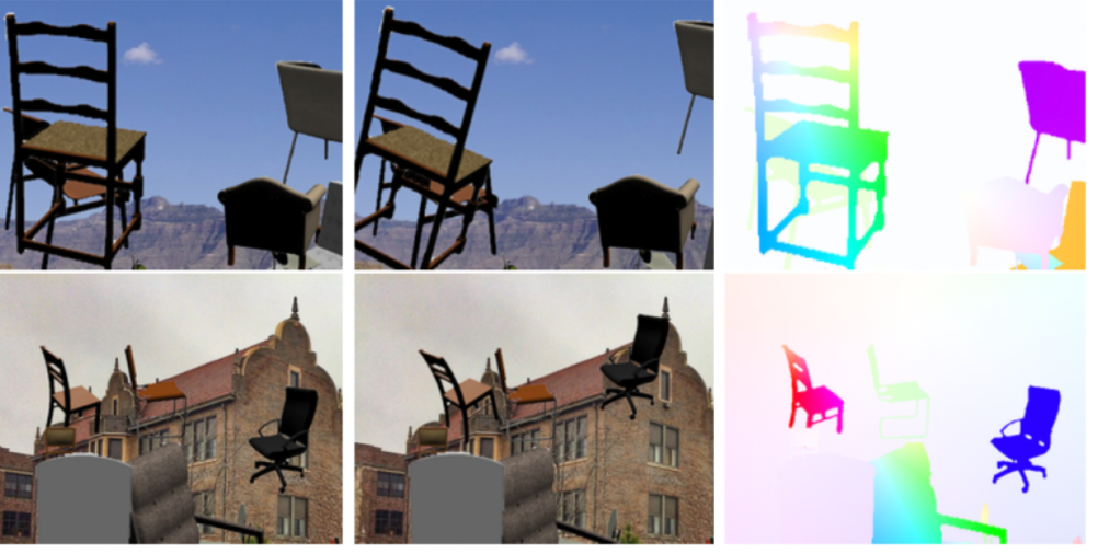
- generate dataset with labelled/ground truth optic flow using game engines
An example dataset that comes out for this is the falling chairs
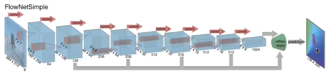
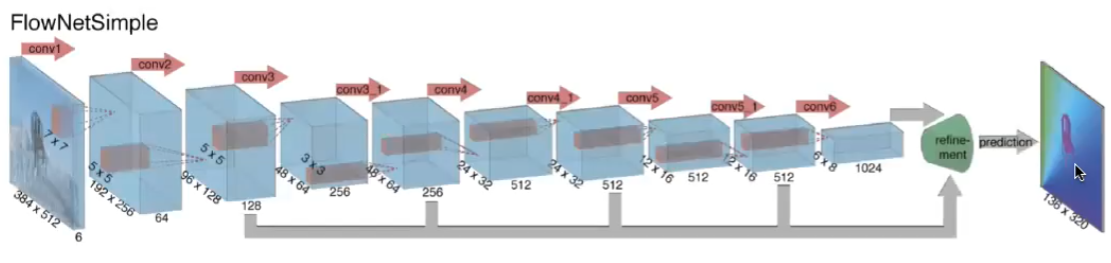
And one model that worded well is the EpicFlow
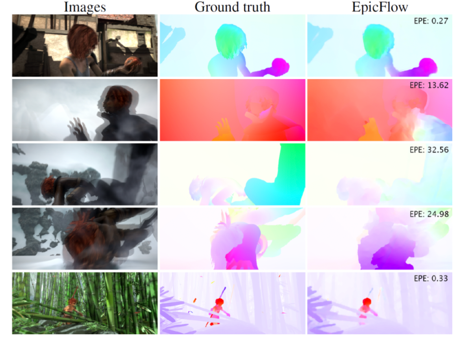
The general setup would looklike:
- input image pairs, output which pixel moves to where (i.e. flow vector for each pixel)
- sample architecture with CNN looks like
Then this can be used to to predict motion by using the motion field
-
Motion Magnification: since machines can see more subtle motions, we can create videos with those magnified
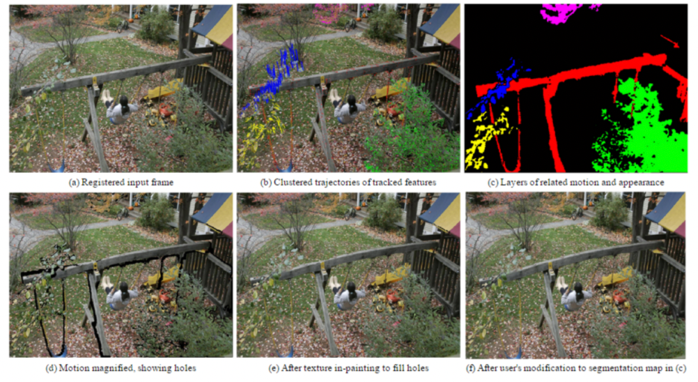
- find the motion field
- cluster similar trajectores
- magnify the motion
Tracking Dynamics
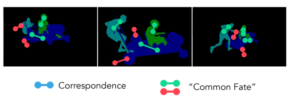
Moving from knowing how each pixel is moving, we would like to consider how each object is moving. Hence we end up in the task of how to track an object.
When tracking an object, we generally consider how to answer the following two questions:
- common fate: connected parts so that they should move together
- correpondance: how do you know those are the same thing after some time?
Example:
The common approach is to solve this by learning an optical flow field using supervised approach. Similar to how we learnt optimal flow:
- given some input video with ground truth labelled object trajectory, for instance
- learnt the tracking
Then you would end up using similar architecture for learning optical flow. For instance:
while this does work great, but the problem would be collecting those labeled data, and that:
Is there an approach where we can solve this without having a supervised approach? It feels that every living being in existence should be able to track without a “teacher”.
- for most problems, if you have a big enough dataset, then they can usually be solved by many architectures
- can we come up with a unsupervised problem that tricks the machine and actually solves the actual problem?
An example would be:
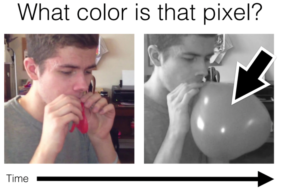
where notice that to answer this question, you would have logically tracked the image!
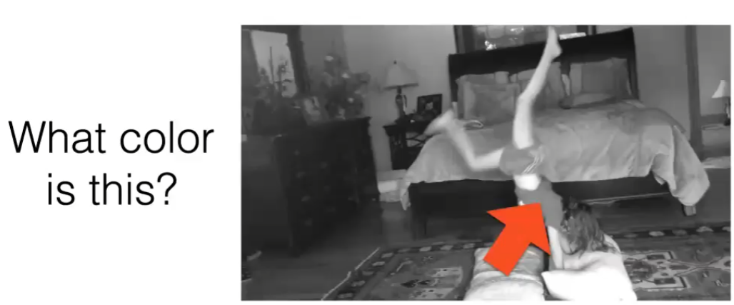
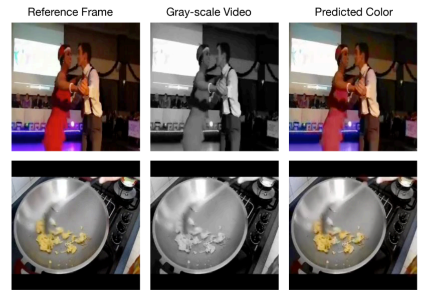
Then we can have a system such that, we are given a colored video:
- only take the first image as colored
- the rest we process to grey scale and feed into network to predict color for each pixel
- notice that we have all the labels already!
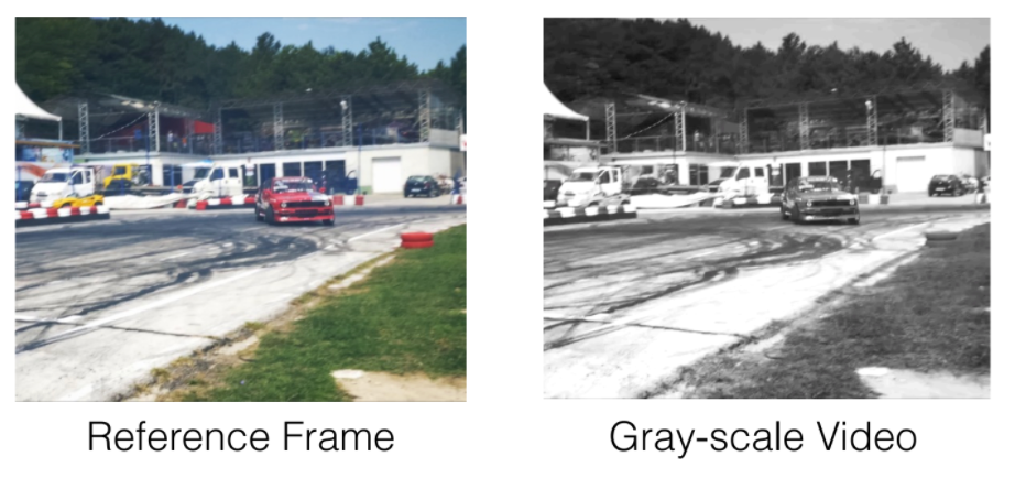
note that this won’t solve the tracking problem conpletely, but is a good approach.
- exceptions inclued an object changing color over time, perhaps due to lighting, e.g. at party house
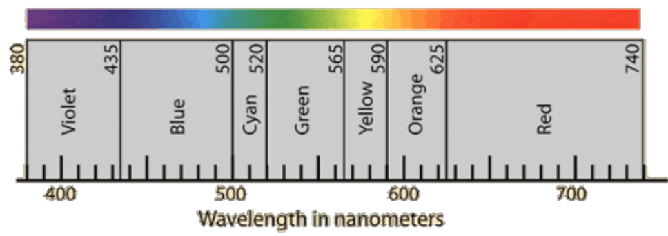
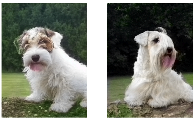
Human Perception of Color
Recall that colors we perceive essentially is determined by wavelength in light
And we have in brain rods that perceive brightness and cones that perceive those colors
| Cones and Rods in Human | Absorbance Spectrum |
|---|---|
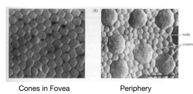 |
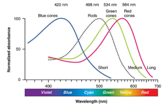 |
where in human,
- we have only three types of cones: one for blue, one for green, and one for red. But combinatinos of the three gives us perception of a spectrum of colors. This is also why we have RGB scale in computer images.
- we have only few cones in periphery, so we are actually not that good at detecting colors at periphery
Then from this, you also get modern applications in how to arrive at different colors:
| Additive | Subtractive |
|---|---|
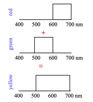 |
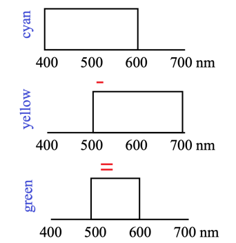 |
- additive color mixing: adding RGB to get more colors
- subtractive color mixing: multiplying/intersection of color
And we have different representation of color spaces
| RGB | HSV | Lab Space |
|---|---|---|
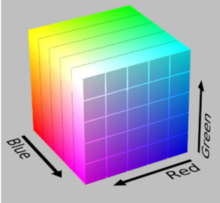 |
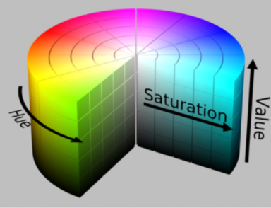 |
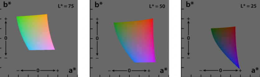 |
where:
- HSV: hue saturation value
- notice that we get an illusino of magenta which comes from mixing of red and blue, which if you look at the wavelength scale, it should not happen
- $L$ in lab space means intensity. This is a non-Euclidean space that seems to correspond the best with human vision (the idea is color spectrum could be a function of intensity as well)
- so essentially $L,a,b$ would be the values for color
- in practice $L$ is often represented as the pixel value when in grey scale
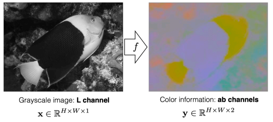
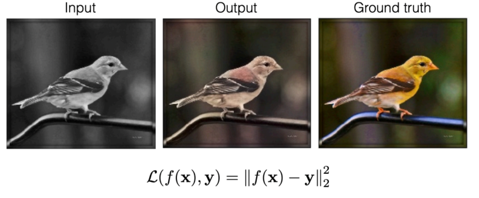
Then using Lab space could be used very commonly in for the task of image colorization
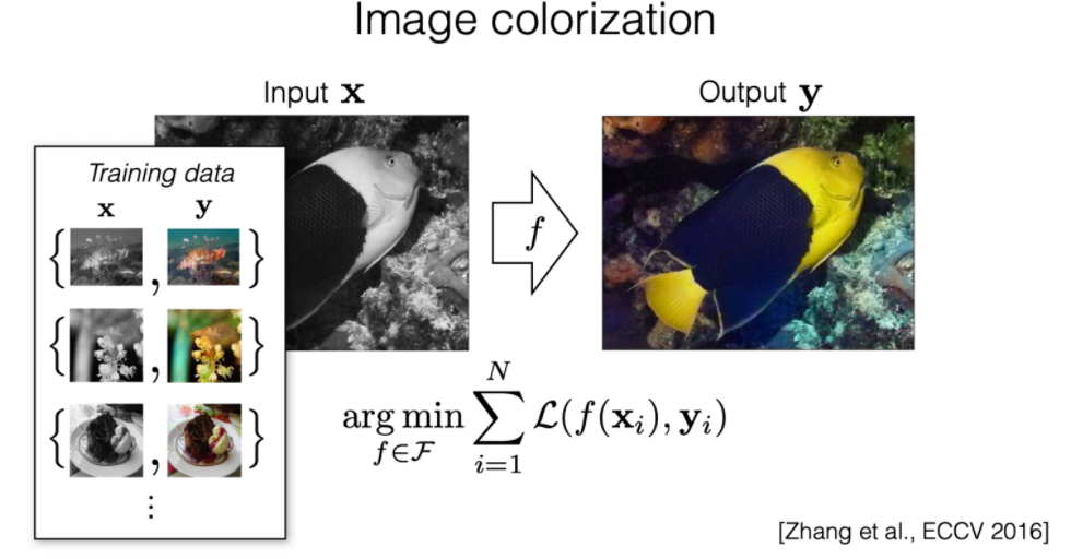
where the:
-
the grey scale image could already be the $L$ values
-
then the task is just to predict $a,b$ values of the lab
We can also only look at the predicted $a,b$ values:
But since we are learning via regression, we could have averaging problem where if we have red/blue/green birds, then
| Given Data | Output |
|---|---|
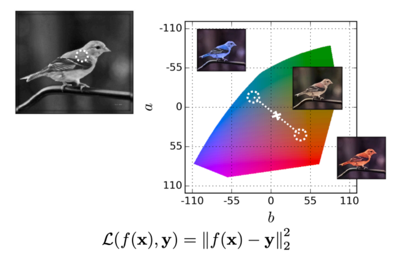 |
 |
One way to deal with it is to predict a distribution of discrete colors, so that we allow for more than one answer!
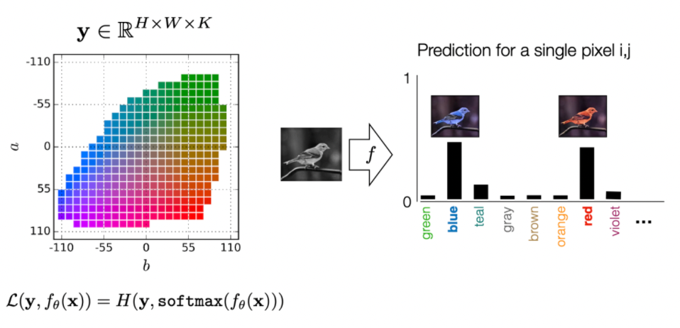
then basically we can output a distribution of possible for color for each pixel.
But still this type of model still have problems in biases:
| Training Data | Input | Color Prediction |
|---|---|---|
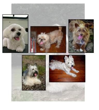 |
 |
 |
where:
- because many training data had dogs sticking tongues out, it paints a tongue as well on the input
Color Mapping for Tracking
For image colorization, we ask the question:
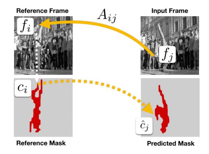
However, in video, recall that we would want to consider coloring for the hidden purpose of tracking. Hence your question would be:
Where should I copy this color from?
| Learning Task | Label |
|---|---|
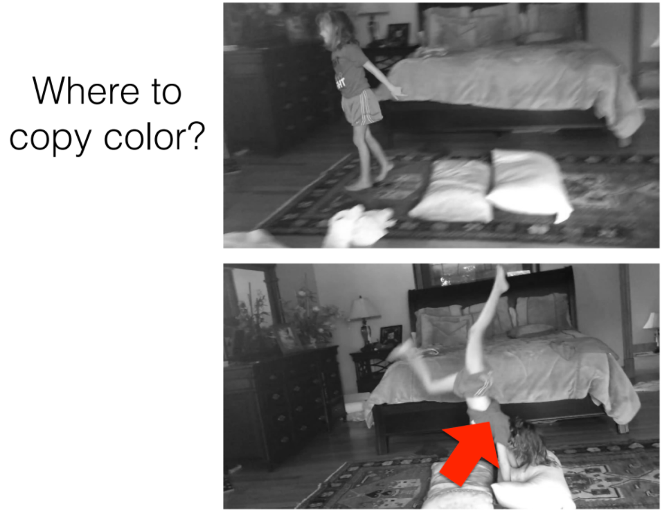 |
 |
where notice that the solution to this colorization problem is tracking (hence we achieve our goal)
- we do not want to say that all objects of the same color are the same object, which is kind of what image colorization do
- here we learn color for tracking, hence this reformulation.
How do we color the video such that it learns where to map?
- essentially what the NN learn is a pointer, but the loss is on the color
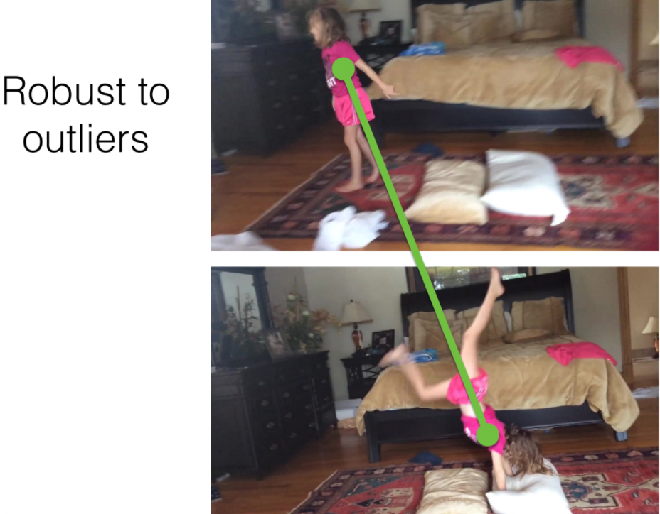
For each pixel, we have some embedding.
- $i,j$ would represent the location of the pixel in each image
- for every pixel $i$ in frame 1, we want to know how similar is it (i.e. if same object) to pixel $j$ in frame 2, e.g. at a later time.
- Hence we get a matrix $A_{ij}$ for measuring similarity between every pair of pixel
- then, we want to assign same color to “similar” pixels by having a weighted sum
Therefore, the whether if a pointer exist between pixel $i$ and $j$ would be represented by similarity between $f_i$ and $f_j$.
Graphically, we are doing:
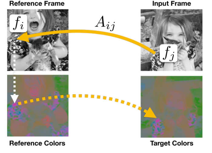
In more details: given color $c_i$ from reference and (learnt) embedding $f_i$ from refernce, and a input to predict, what is the color at each position $j$? We do this by:
\[\hat{c}_j = \sum_i A_{ij}c_i,\quad A_{ij} = \frac{\exp(f_i^T f_j)}{\sum_{k} \exp(f_k^T f_j)}\]essentially a weighted sum based on similarity of the embedding of each pixel. (note the analogy to self-attention mechanisms)
Then since we have the label already:
\[\min_\theta \mathcal{L}\left( c_j, \hat{c}_j | f_\theta \right) = \min_\theta \mathcal{L}\left( c_j, \sum_{i}A_{ij}c_i \,\, |f_\theta \right)\]so that
- for a particular video, our NN would be able to produce a pixel-wise embedding $f$ from its learnt parameters $\theta$
- once we have the embedding, we can color the image or we find object correspondance hence tracking by measuing similarity between $f_i,f_j$ between any two locations of between two frames!
Example: using it to predict color
which implicitly learns object tracking. Therefore, if you need tracking information, you just keep a pointer by:
-
compute the $\arg\max_{i} f_i^T f_j$ so we know which pixel $i$ the pixel $j$ corresponded to
-
then convert an entire group of it as a mask
and let the mask propagate in your network to do other things. Some more result examples
| Tracking Segments | Tracking Poses | Visualization of Embeddings |
|---|---|---|
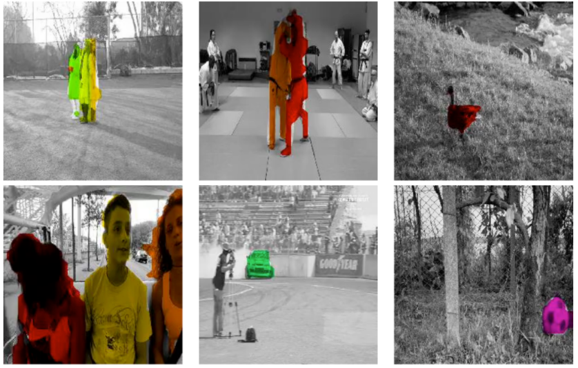 |
 |
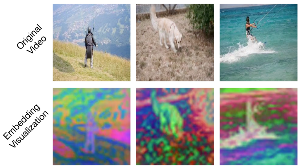 |
where
- embedding in the third example refers to the $f_i$ for each pixel. Since $f_i$ is high dimensional, we needed to use PCA to reduce it to 3 dimension to superimpose on the original image. Note that this could also be useful for drawing a segmentation for objects in a video.
- note that the above notion of $\arg\max_{i} f_i^T f_j$ makes sense as the colors we found is dependent on the similarity between $f_i$ in input/reference image and $f_j$ of another frame
Interpretability
How to interpret deep learning architectures? Consider the simple example of
What are neurons in the network learning? What should it learn?
- those techniques below could also be useful for debugging your model.
This is an important chapter that covers many common technique used in real life to visualize what is happening in your model.
Grandmother Neurons in Human
It turns out that research shows there are specific neuron in your brain that represents your grandmother, a neuron in your brain that represents your friends, etc.
- done by inserting electrodes into brain and letting patients look at certain images. Hence recording neuron activities.
- recall that brain sends electrical signal around. Here it is sticked in visual system, so it responds to what people see and activates certain neurons.
When flashing pictures of celebrities, there are neurons that would only fire for them:
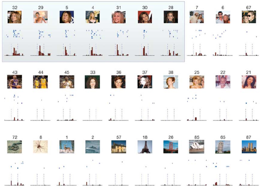
where we see there are high activations for only a few neurons.
More interestingly, they are firing for the concept of a person:
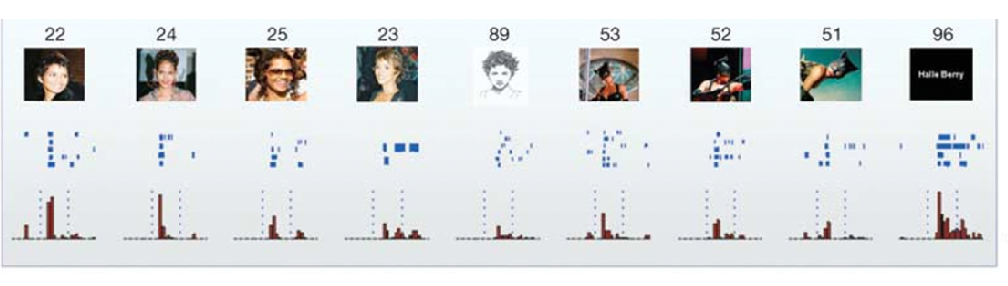
so that it also fires for things like “sketches” Halle Barry.
- but the question is, if I take out that neuron, would I forget about Helle Barry? It is highly plausible that there would be redundancies in brain so that we don’t forget easily.
- but still the concept of a few/specific neurons being able to fire/activate for a certain class is important.
A grandmother neuron is a neuron that responds selectively to an activation of a high level concept corresponding with an idea in the mind.
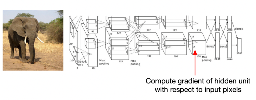
Deep Net Electrophysiology
Following from the above search, this hint on one way how we can interpret deep learning networks, by looking at what kind of image patch would cause the neuron to fire.
- other interpretation methods include Similarity Analysis, Saliency by Occlusion, etc.
First, we consider the activation values for each neuron:
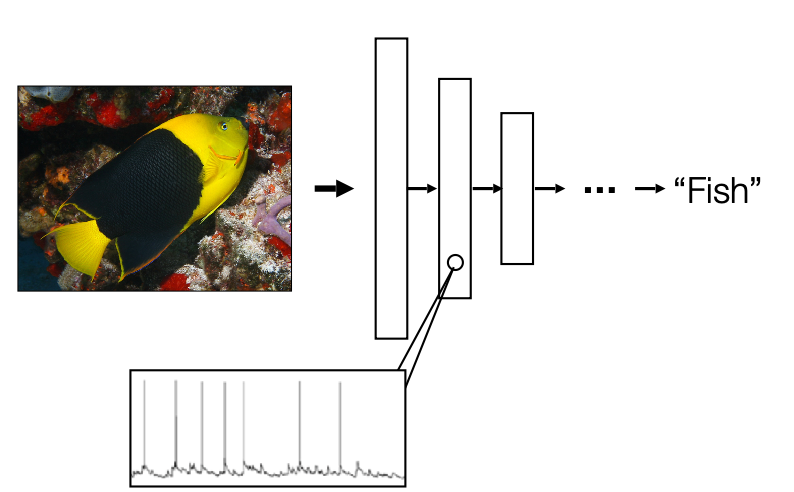
then you can also get a graph like the above for a certain layer.
A more detailed example is visualizing the CNNs. Here we have each layer being a bunch of Convolutions, and we treat the kernel as neurons.
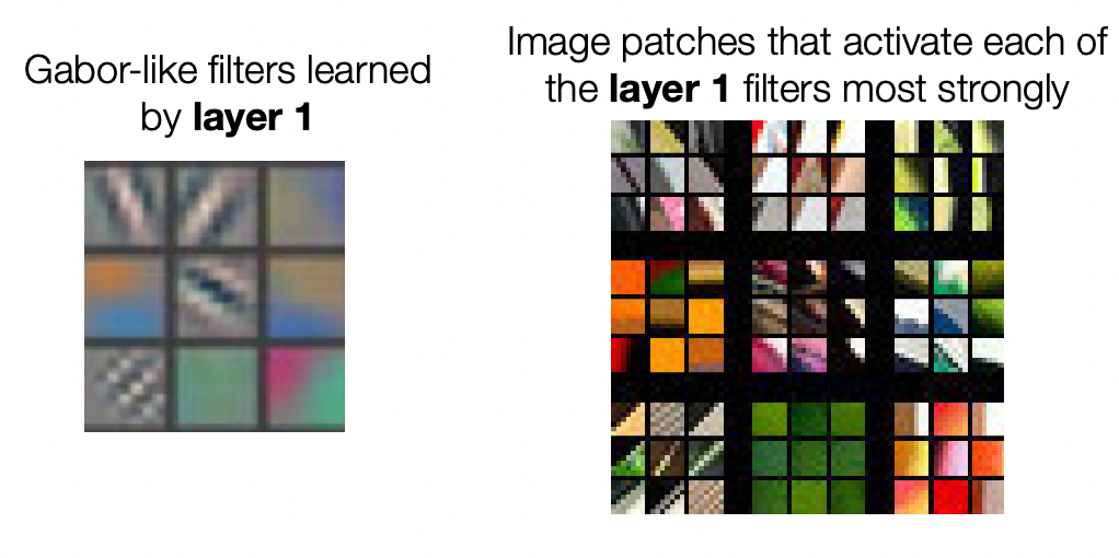
where essentially we record what image batches activate the first layer most strongly, and it seems that we are detecting edges. If you also do it for layer 2 in the network:
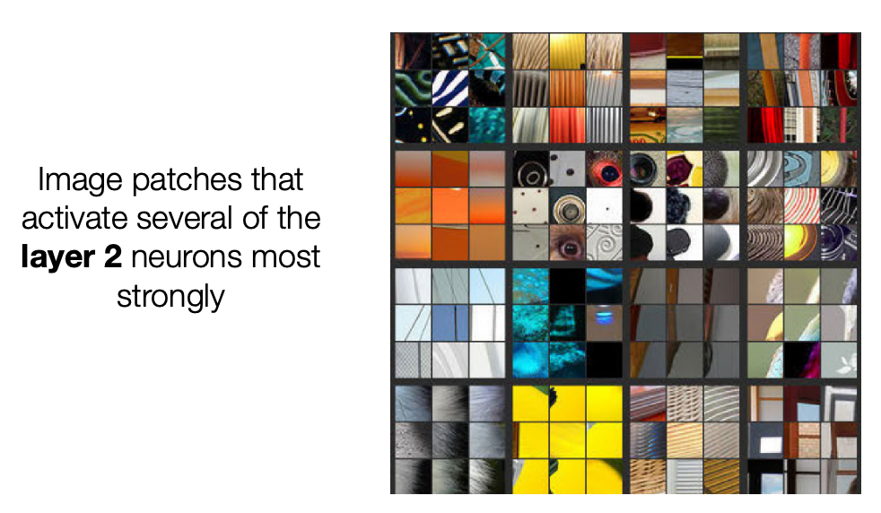
where it seems that those neurons are firing for patterns/shapes, and finally at layer 3:
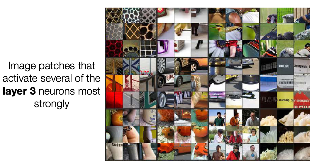
where here we seem to be able to put shapes together and detect objects!
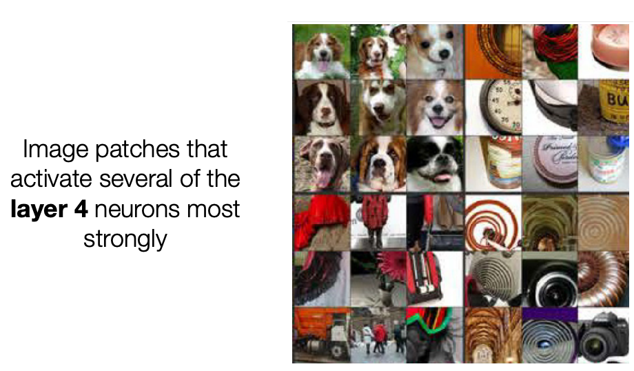
and etc. But notice that the image activated are axis aligned
Since rotations are linear transformation, then we should imagine that to not change any information hence learnt representation should have an arbitrary aligned axis?
- rotation can be performed by a linear transformation, so then a NN could have rotated and those representations. Then why are we still have the vertical alignment for maximal activation? i.e. the activation is lower if we rotated the image, which shouldn’t happen.
Therefore, this also motivates another view that instead of having a grandmother neuron specialized for a concept, could it be that we have a distributed view of a concept across neurons, so that the combination gives us the classification?
- then we can perhaps recover the extra degree of freedom carried in by transformation such as rotation?
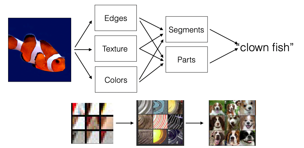
In summary, it seems that CNNs learned the classical visual recognition pipeline
We can also quantity this at each level:
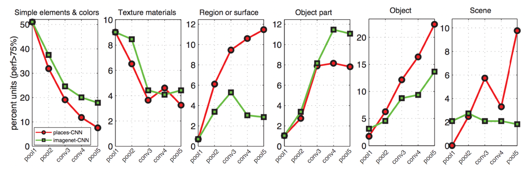
where vertical is percent of neurons that activated when pictures described in the title is fed in. So here we see that:
- the deep layer we are in the model, the more higher layer concepts we are leanring.
Similarity Analysis
Then if we take the embedding vector/hidden state of those images, we can also compare those vectors between images of different classes:
where we expect that similar images should have similar representations. Then we can use this to conpare compare thi
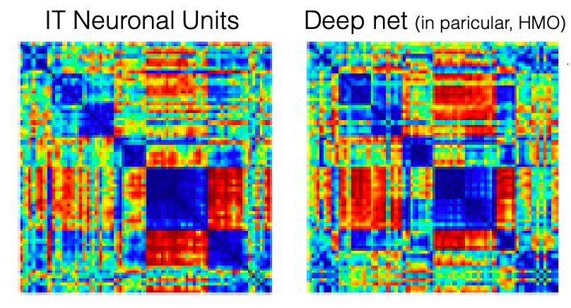
where here we can see what DNN thinks are similar or different objects. The correspondence (left is from people) is high!
- in some ways, this is surprising that machine is learning a similar way as human does
- but it could be reasoned that as humans are labelling those images. of course machines learnt a similar way.
Saliency by Occlusion
What part of the image does the neural net make decisions on? Which part of the elephant did the neural net use to determine?
One simple idea is to blocking of several regions in the image, and consider how much does the score go down when each region is blocked
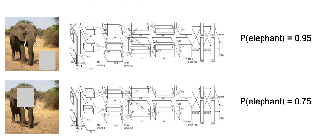
Then doing it over all regions:
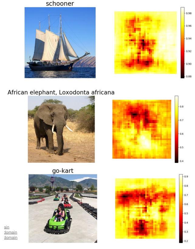
where we can basically identify:
- which part of the image blocked out, still has high confidence
- then the inverse of the number would represent importance
Another intuitive approach would be to answer the following question.
What is the maximum number of pixels I can mask out so that the machine can still classify the image?
An example of answering the above question would be:
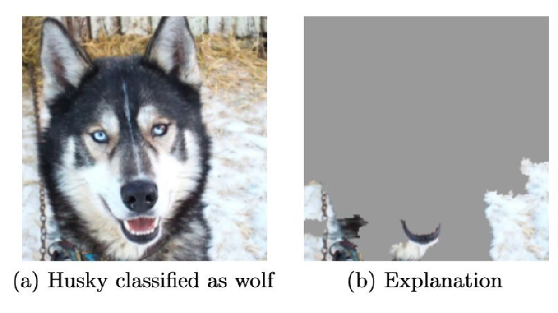
so in this case the neural net is not learning the correct thing.
Guided Backpropagation
What pixles can I twiddle such that the resulting clasification is no longer correct?
Then this results in
Guided backprop: Only propagate pixel if it has a positive gradient backwards, i.e. activation increases if this pixel changed. Truncate negative gradients to zero.
- the reason why we truncate negative gradients is because we want to find which regions cause the object/find causation relationship, not the regions that do not cause it.
Visual examples of what we are doing:
Results:
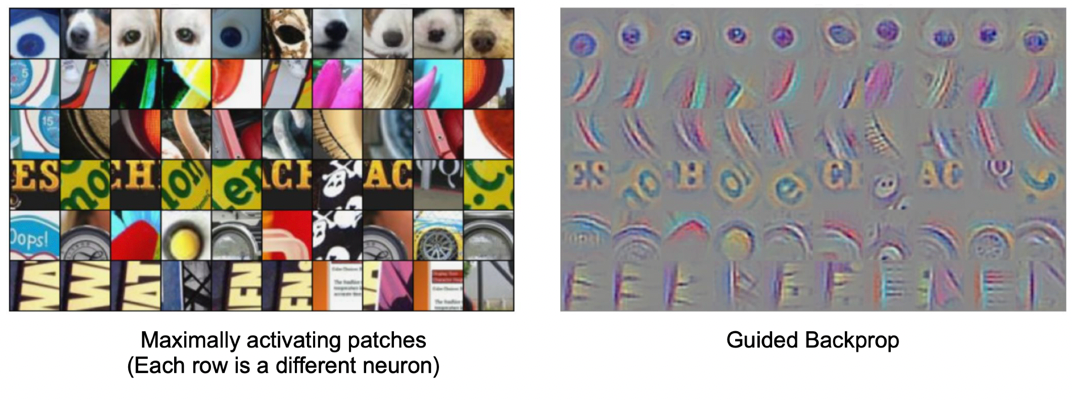
where in this result, we are doing:
- patches found using the “Grandmother” neuron procedure, i.e. maximum activating patches
- from those patches, we perform a guided backpropagation to know what aspects of those patches that caused the maximum activation
You could also do only a guided backprop on the whole picture.
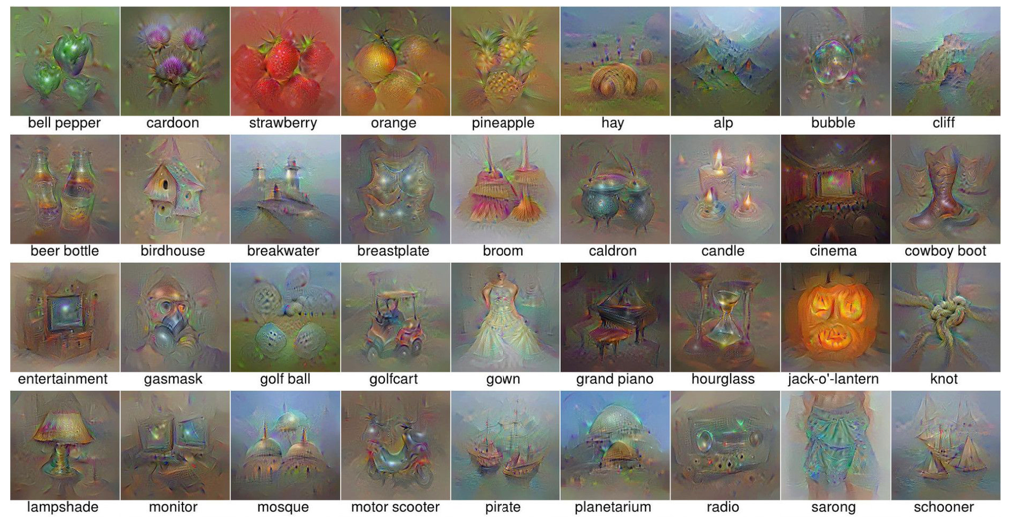
Gradient Ascent/Adversarial Attack
Given a trained model, what image does the network think is the most representative/likely of class $k$?
Then we consider:
\[\max_x f_{\text{neuorn}_i}(x) - \lambda ||x||^2_2\]where $f$ would be the activation function for each neuron
-
$x$ would be input to each neuron, which corresponds to certain pixles of the image
-
the regularizatoin is needed so that $x$ would be at least in the visible range, as otherwise we can go towards infinity
Then eventually we do a gradient ascent to find the “best representation for each class”. Results look like:
Then the “fun” things people could do is that we can try to modify an image such that some class $k$ would be activated for a neuron:
| Original Image | Modified Image using Gradient Ascent |
|---|---|
 |
 |
where in the right we are modifying images so that the model would have triggered activations of many classes you like.
Self-Supervised Learning
One example we have seen before would be how to use color for tracking, which turned the task into a self-supervised/unsupervised task. Here we see some other generic unsupervised methods used for downstream tasks.
-
such as unsupervised segmentation $\to$ object detection.
-
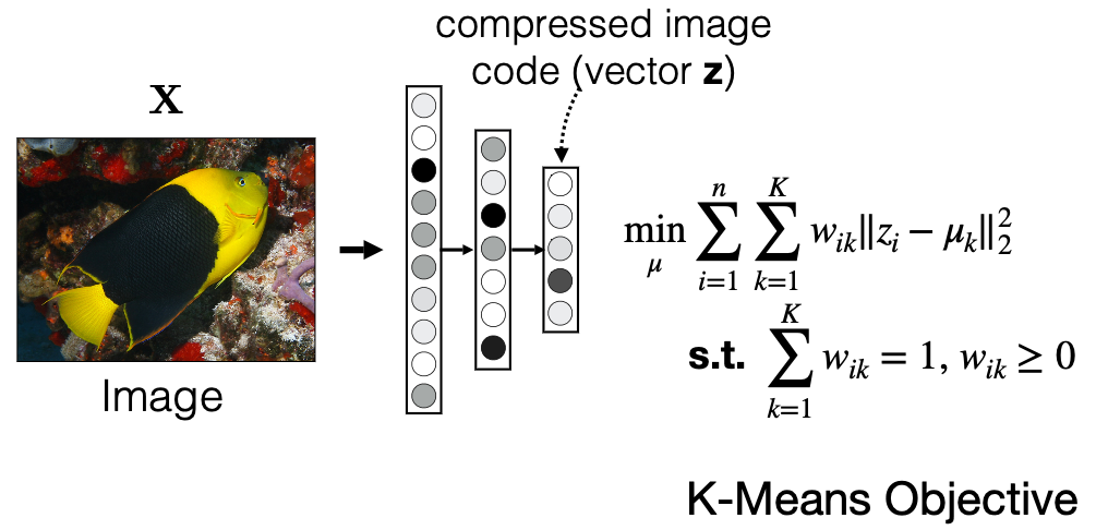
e.g. representations learnt can then be used for clustering. We can use the learnt $h=z$ hidden vector for k-means
One simple architecture used would be similar to the process of fine-tune a pretrained model:
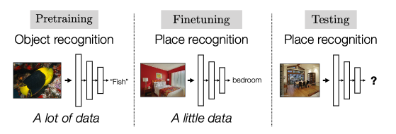
where the key point is that finetuning starts with some representation learnt from a previous task hence:
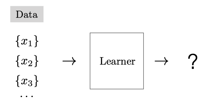
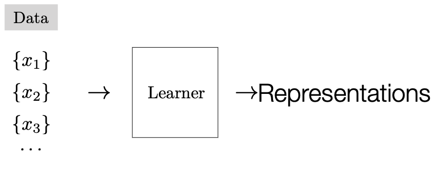
- we aim to construct a network that can learn useful representation $h$ of images $x$ in an unsupervised way
- then use that representation $h$ as a “pretrained network” for fine-tuning on other tasks
hence here we are mostly concerned with:
| General Self-Supervised | Self-Supervised Representation Learning |
|---|---|
 |
 |
Why is having some representation $h$ useful?
Consider the example of remembering the observed image and then drawing from scratch
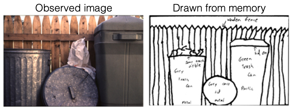
notice that:
- when most people draw it, we automatically extrapolated: we drew the entire rubbish bin when we only observed part of it
- the same happened for videos, when we are only show part of a video and were asked to describe it, we extrapolate unseen scenes.
Our mind is constantly predicting and extrapolating. Self-supervised learning aim is to be able to extrapolate information/representation from the given data.
Common Self-Supervised Tasks
How do we get that representation $z$ or $h$? Here we will present a few:
- find a low dimension $h$ such that reconstruction is the best: autoencoder
- find a network $f_\theta$ that outputs representation of both image and audio of the same video, and maximize correlation
- find a network $f_\theta$ that outputs representation for context prediction, i.e. predicting relative location of patches of an image
- find a network $f_\theta$ that outputs representation that can be added, i.e. sum of representation of parts of an image = representation of an image
- find a network $f_\theta$ that outputs representation such that similar objects in a video have a similar representation
Using Autoencoder
One self-supervised task is to use an autoencoder to learnt $z$ for reconstruction:
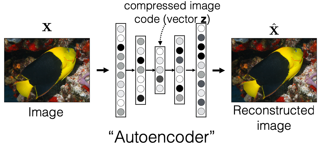
where the loss would be reconstruction loss $\mathbb{E}[f_\theta(x)-x]$. of course you want to make the dimension of $z$ much smaller than the dimension of the image. So you want the representation to be reflective of the object
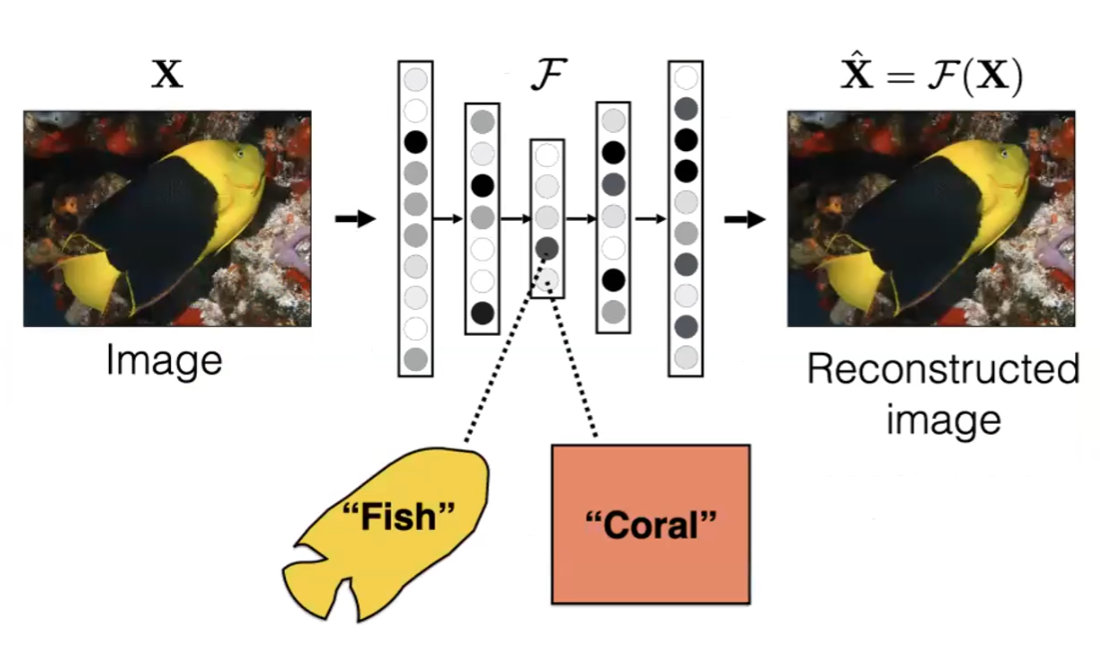
e.g. we hope that $z$ can compress and learn “face of fish is yellow”, etc, but in reality is just learnt a down-sampled version of the image
Using Audio Data
Another idea is correlate different views of the data, and hence predict “what sound it can produce” (this is actually one of the first self-supervised approach).
- hence, rather than compression, this is about prediction/extrapolation
- i.e. I know what a “cow” is because it can make a “moo” sound. Hence the representation should reflect the two
For example, given an input video, it will have both sound and image in the video:
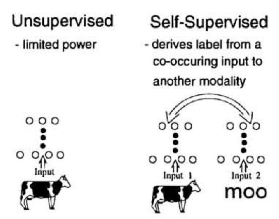
where our aim is to let the model be able to say that “cow” produced the sound “moo”. In fact, this idea itself to use different modality of the same data is common in self-supervised learning in CV (e.g. colorized image vs grey scale)
Using Context Prediction
we want to improve the autoencoder so that it does not just learn a down-sampled version. Consider solving the following problem
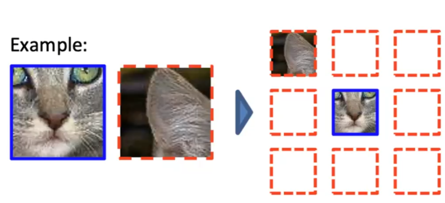
notice that to solve it, we needed to know how a cat looks like.
Hence, we want to predict the spatial layout between the patches, which depends on learning some good representation $z$ of the object:
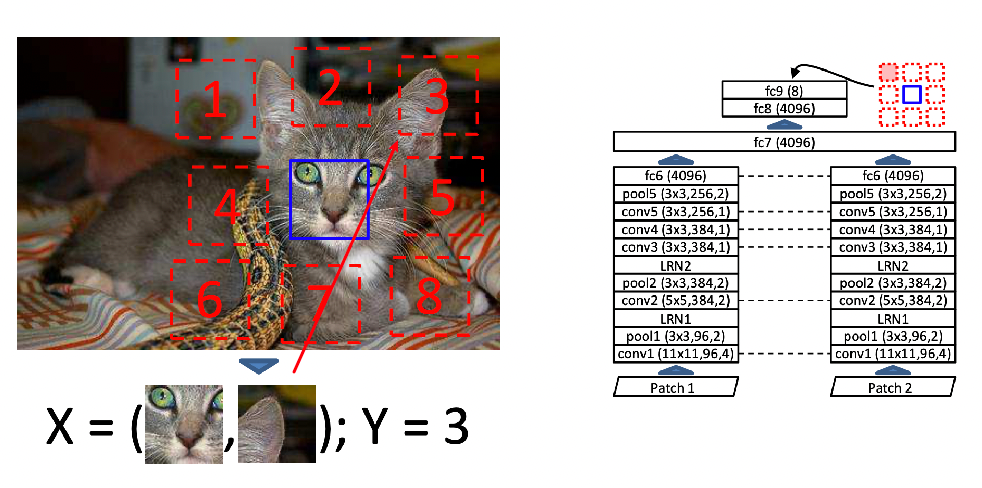
where remember that instead of just compressing the image. it should manage to learn “what a cat looks like” so be able to correctly place the missing patch:
- note that then context prediction, the $Y$ we already know as we have the entire image. Then, since we only have 8 choices of where to place it, the loss would be cross-entropy loss
- similar for image colorization, the by-product of this would be a neural net that produced $n=4096$ vector $h$ which should be representative of the image patch
How do we visualize the embeddings $h$? One way is to do:
- given an input patch $i$, produce an embedding $h$
- find nearest neighbors $j$ of the that embedding amongst the training data
- return that original image patch $j$
Some examples:
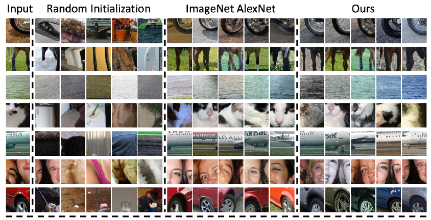
where notice that:
- the AlexNet representation also learnt the color of the wheels, but the new version learnt only the wheel
Using Counts
Another idea is inspired from counting: i.e. the sum of the representations should recover the total representation:
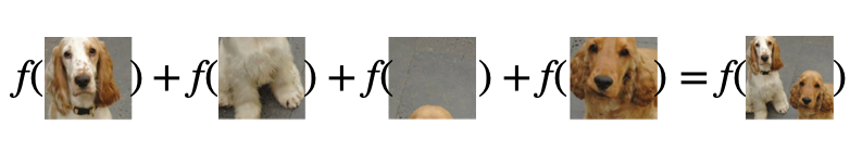
the intuition is we want to leverage recursive structure to images:
- consider the question being how many eyes there are in the last image
- it should be the same as the sum of number of eyes in those 4 patches
Hence the architecture is
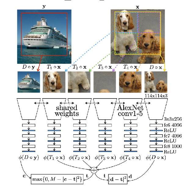
where
-
first we concatenate the four pieces into $t$
-
you want the sum to be close to the original image $\vert d-t\vert ^2$ but far away from some other random image $-\vert e-t\vert ^2$
This is very valuable in videos as we want tracking objects which can easily deform, e.g. a human doing parkour.
Using Tracked Videos
We can use this idea of the same objects in a video over time should be close to each other in the embedding space, even if its shape could have deformed:
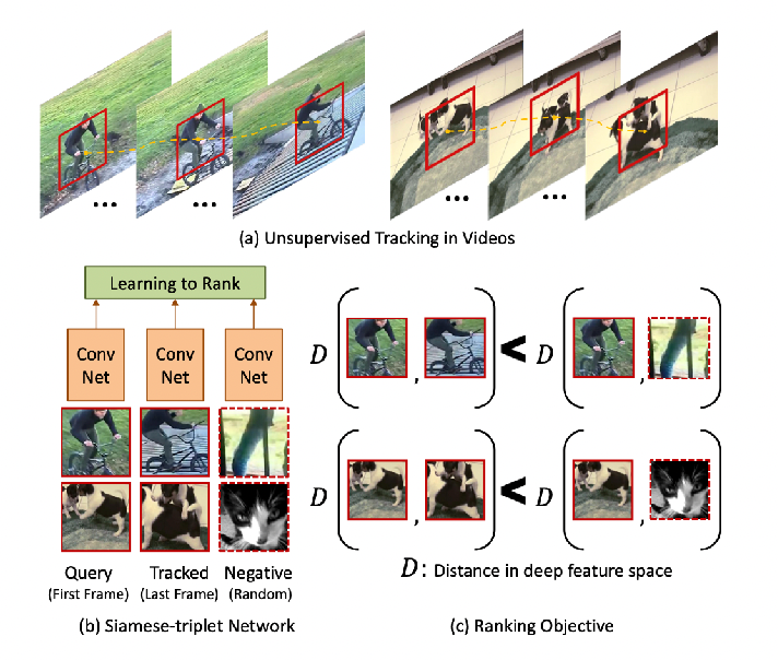
where
- this of course requires an already labeled/tracked video
- again, we want same objects being close but different objects being far away
Learnt Kernels from Unsupervised Learning
In many of the above applications, we can visualize the kernels learnt:
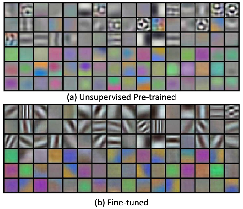
where notice that they ended up learning a very similar kernel than fine-tuned tasks which is a supervised version.
Contrastive Learning
This is probably the most successful unsupervised learning method in CV to date.
The idea is the following:
- given an image, we can create its similar pair by transformation of itself such as rotation/cropping
- given an image, we can create negative pair/different pairs by transformation of other images
- given any of the two images above, we also want to encode it $h_i = f(x_i)$ using an encoder
Then, we want to minimize the following loss:
\[l(i,j) = -\log \frac{\exp(\text{sim}(z_i,z_j) / \tau)}{\sum_{k=1,k\neq j}^{2N}\exp(\text{sim}(z_i,z_k) / \tau)}\]essentially making sure that similar pairs score high (e.g. same labelled pair). Of course this can be extended to learn negative pairs as well (SupCon). Graphically:
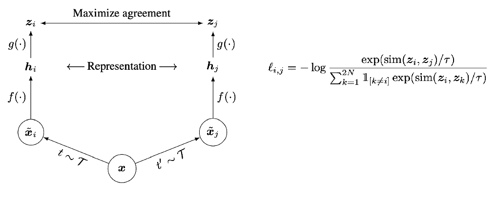
where:
-
we want the network to agree that they are the same object/representation if it is just rotation/cropping of the object
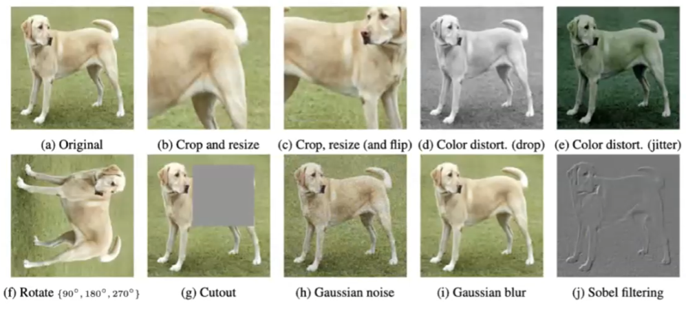
-
the loss have $z_i,z_j$ being the same image, $z_k$ is iterating over all images. Hence we want the top to be as small as possible/close together, while the denominator we want to be large/far away
Notice that the loss is on another representation $z$ rather than $h$ which is the representation we use. The idea is that $z$ vector might only be storing the minimal sufficient part of the image for maximal agreement.
However, this does perturn the objective of “ensuring $h$ representation is good” as ensuring $z$ matching might not be enough. But empirically it works.
Finally, when training is done, we can take that $h_i$ for each input image $x_i$ and plot them (not on this dataset, just for example)
| SimCLR | SupCon |
|---|---|
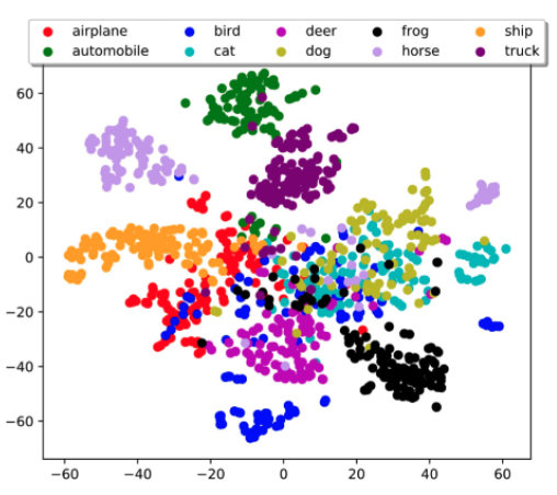 |
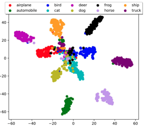 |
so that essentially close together pairs seems to be clustered.
This is very as it even beats some of the supervised version:
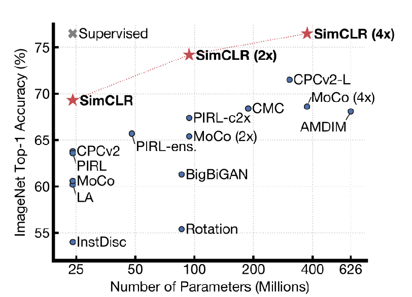
Causal Interpretation
see https://arxiv.org/pdf/2005.01856.pdf
Learning Visual Shortcuts
Whether if this is a good phenomenon or bad depends on how you use/see it. Consider the task of recovering the layout of an image:
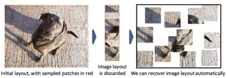
which works well as an unsupervised task. However, if we convert the image into grey scale, the same training image failed:
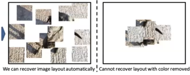
why did that happen?
- this is because there is chromatic aberration and vignetting in the inage, where neural network picked up as clues.
- however, those are hidden information relative to human eyes
Chromatic Aberration and Vignetting
Those two are come from the physics of lenses, essentially its property that refraction depends on the wavelength of the light.
Chromatic aberration, also known as color fringing, is a color distortion that creates an outline of unwanted color along the edges of objects in a photograph.
Vignetting is a reduction of an image’s brightness or saturation toward the periphery compared to the image center.
| Chromatic Aberration (exaggerated) | Vignetting |
|---|---|
 |
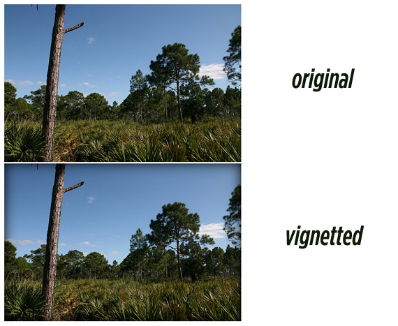 |
Why did they happen?
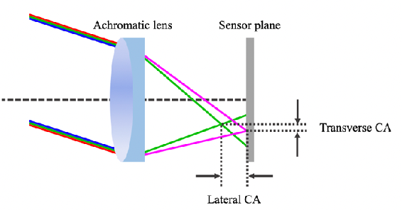
- the fundamental problem is it is difficult to focus on all wavelength in the same manner using a lens
- so that some wavelength, e.g. purple, got focused better than other color, such as green, causing chromatic aberration
- on the other hand, more light is going through on the center, hence in general you have brighter regions in the center - cuasing vignetting
Graphically:
| Causing Chromatic Aberration | Causing Vignetting |
|---|---|
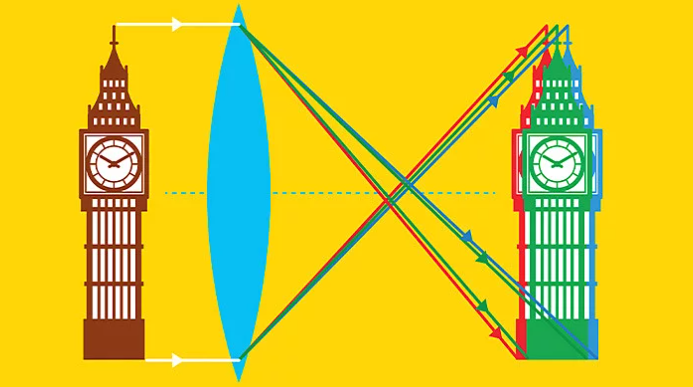 |
 |
Using Shortcuts
Hence NN utilizes those to do patch re-localization. Some plots of how those effects affect performance:
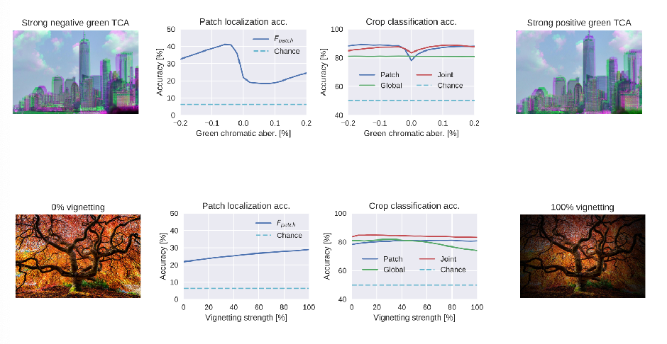
But you can also turn this as a good “feature” of the program, as chromatic aberration and vignetting is always present in photos, we can use it to detect if the photo is cropped/edited/etc
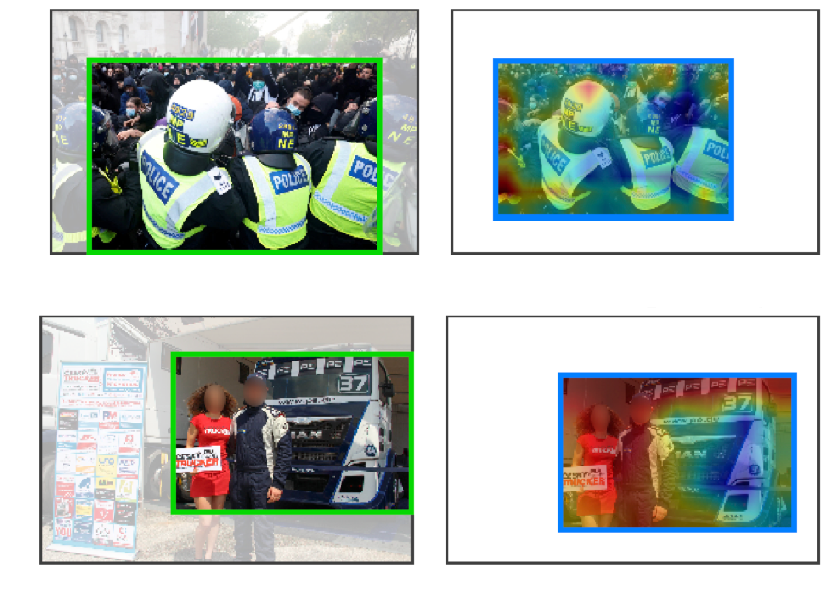
where, for instance, if the photo is cropped, then the vignetting/chromatic aberration center will be shifted.
To Reinforcement Learning
Self-supervised learning sounds like the “next stage” for supervised learning. But there could be more
Kitten Carousel:
Consider the following experiment:
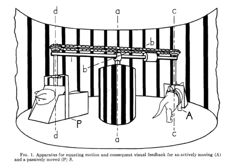
- take two cats born in darkness, and let them grow up in darkness
- the first cat $A$ can move around and see scenes
- the second cat $P$ can not move, but they are seeing the same thing as the contraption is symmetric
- then they did some IQ test on both cats afterwards, and it turns out that cat $A$ is smarter (though this result is very controversial)
The upshot of this is that ML algorithms is essentially cat $P$, it is not interacting with the world, only learning from observations.
Hence then we get the field Reinforcement Learning becoming a very important field for building intelligence.
Yann LeCun’s cake
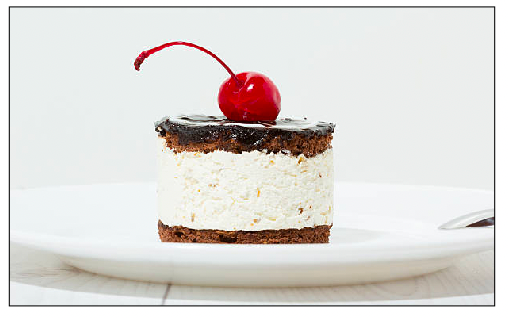
- Cake is unsupervised representation learning (i.e. most of the math)
- Frosting is supervised transfer learning (we need a little bit of it to be interesting)
- Cherry on top is reinforcement learning (model-based RL)
so that AI would work with just 1 and 2, but more intelligence needs interactions hence 3. But of course, the third step is expensive as it could have high stakes, i.e. if you make a mistake, people might get hurt.
Synthesis
Before, all the tasks we had could be generalized to “how to process an image”.
The goal of synthesis is “how to create an image” (either generate from scratch/random noise or manipulating existing ones)
Some history of photographs:
In 1888, when the first camera is created, photos were proofs. However, that only lasted 100 years:
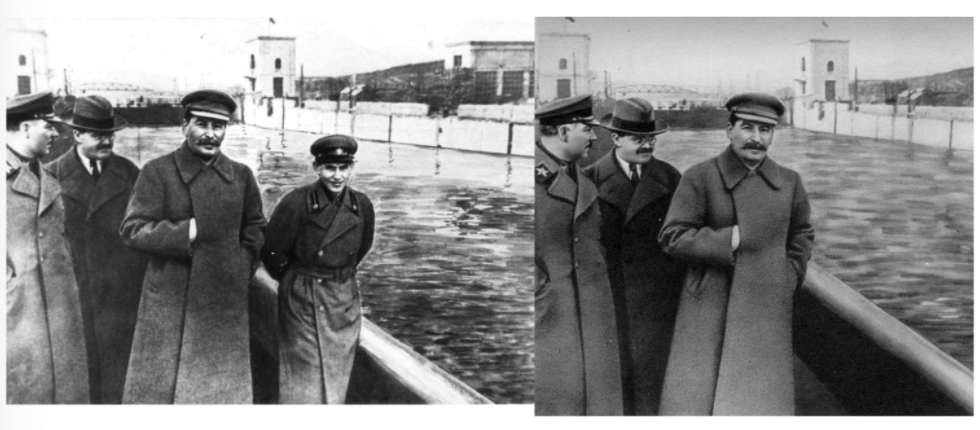
which comes to the topic of how to synthesize images, e.g. DeepFakes.
Since we need to create an image, we are moving from discriminative models to generative models
-
Discriminative Models (what we had before, e.g. CNNs)
- Learn the linear/nonlinear boundary between classes
- Estimates: $P(Y \vert X)$ the posterior (which essentially learns boundaries)
-
Generative Models (what we want now)
- Learn the distribution of the data
- Often you can sample from it
- Estimates: $P(Y, X)$ the joint (i.e. learn the data distribution, hence generate more data)
Examples of generative ones we will discuss include
- GAN networks, e.g. trained on many dog samples, and synthesize a new dog, and OpenAI DallE 2
- Variational AutoEncoder
- etc.
View of Generative Models
Of course the aim of genenerative models is to directly learn the distribution $P(X,Y)$. But along with this goal, we need to make sure:
- model being able to inferencce/genereate data within the distribution but outside of training data
- we also want to able to draw samples from it
Hence this results in the following idea for generative models:
Given some known prior distribution $p(z)$, e.g. a Gaussian, learn a mapping (e.g. done from neural network $G$) from $p(z)$ to the target joint distribution you want to learn.
Visually, if we need to find a model $G$ such that it learns:
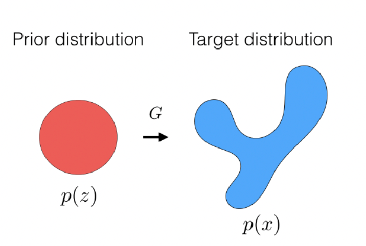
so that for generation, then we just need to give a random input $z \in p(z)$ to $G$, and it will give us a synthesized output.
Then, in eventually you use a NN to model $G$, hence basically genreative models are doing the following:
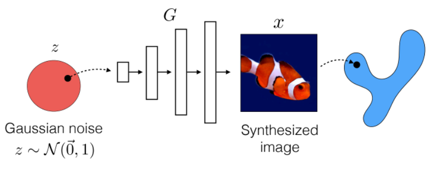
where after you learnt the parameters in $G$
- $z$ input would be input from the prior $p(z)$ you specified in training
- $x$ output could be an image, for instance.
But how do you know that the networks is not memorizing photos? i.e. memorizing $z \to x$ being an identity map?
This is often resolved by the fact that you can move in latent space $p(z)$ and change attributes of a given $G(z)\to x$ such as camera view point. This shows that it can interpolate unseen images, hence not merely memorizing!
Visually, again the aim of learning $p(x)$ from a finite set of training data is to that we can interpolate unseen images:
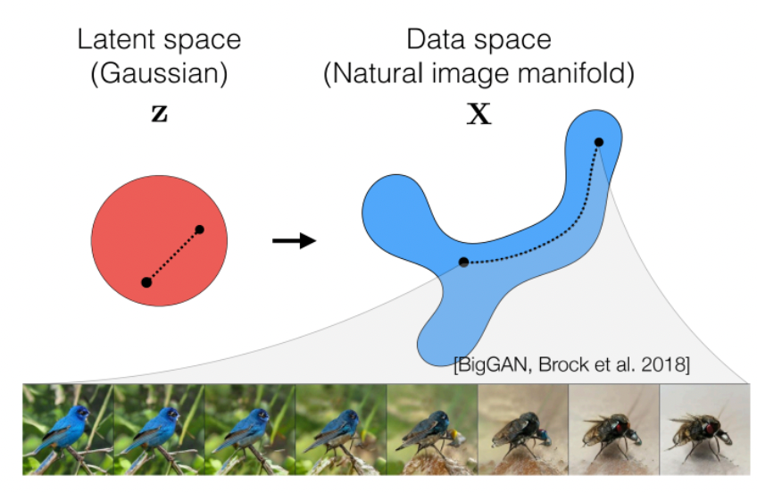
where you can imagine the two black dots being the given training set, data along the line are interpolated.
Additionally, some research shows that, given a $z,G(x)$ pair, you can move along some specific direction (a basis for the Gassian) of the latent space $p(z)$, and obtain samples of data corresponds to changing in camera viewpoint
| Angle 1 | Angle 2 |
|---|---|
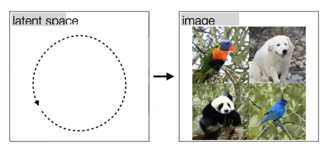 |
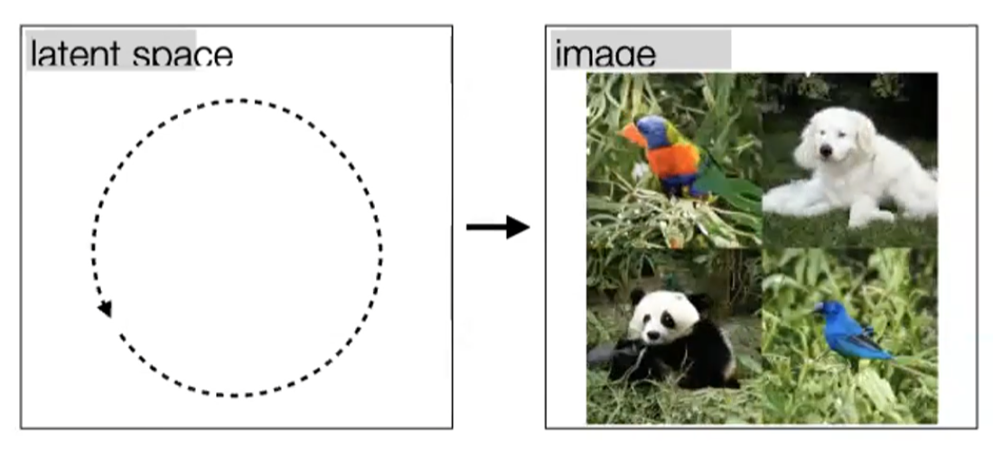 |
In fact, there is a class of GAN network that aims to find ways to, say, change the color only, change the view point only, and etc, which is called StyleGAN.
Generation with VAE
Recall that the classical autoencoder does compression:
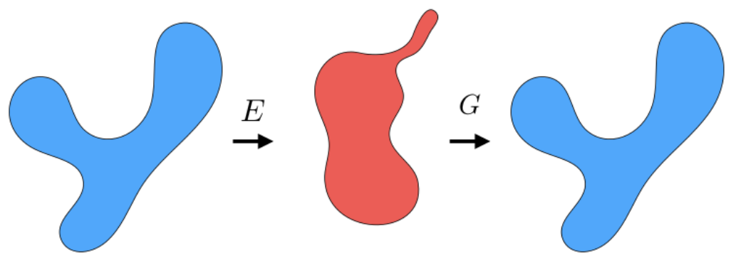
where your model $M$ would learn
- an encoder that goes from $E(x) \to z$ being compressed
- a decoder that goes $G(z) \to x$ seems to learn a mapping from the red space to blue space
But why does pure autoencoder not work? Because we technically still don’t know the red latent space, hence we cannot sample $z$ from the latent space to generate some new data. Therefore, instead of mapping to some random latent space, we can enforce it to map to a known, given prior distribution:
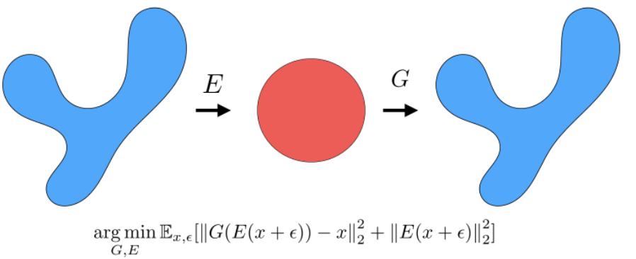
Therefore we consider Variational AutoEncoder:
- we are learning a mapping from prior distribution in red (e.g. Gaussian), which is parameterized distribution (so that we know how to sample from it once we know the parameters) to the target distribution
- then we can construct this problem as an autoencoder like problem, but $p(z)$ would now be parametrized
- with this learnt, we can sample from $p(z)$ and when $G(z)$ to output a new image/sample!
| Learning Time | Generation Time |
|---|---|
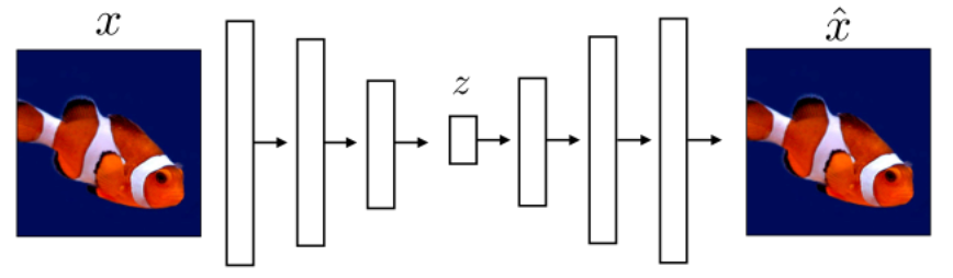 |
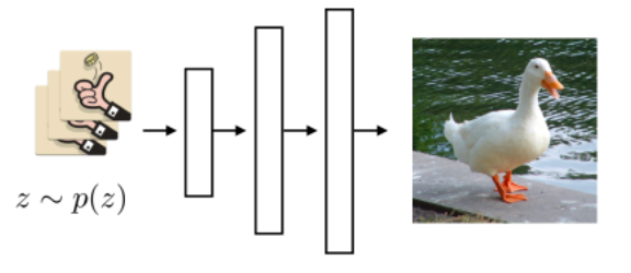 |
Formally, this is how it works. First we consider learing $G_\theta$ that maps from $z\sim p(z)$ to $x \sim p(x)$. Given $p(z)$ which is known:
\[p_\theta(x) = \int p(x|z;\theta)p(z)dz\]then we need to figure out $p(x\vert z;\theta)$, which is essentially given a $z$, how can we map it to a distribution?
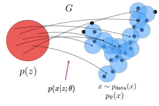
Suppose we can approximate the target distribution $p$ by assuming it to be a collection of priors so that
\[p(x|z;\theta) \approx q(x|z;\theta)\sim \mathcal{N}(x;G_\theta^\mu(z),G_\theta^\sigma(z))\]so that eventually all $x \sim p(x)$ is approximated by
\[x = G_\theta^\mu(z)+G_\theta^\sigma(z)\cdot \epsilon\]for $\epsilon \sim \mathcal{N}(0,1)$.
So essentially, the network $G$ decoder has to learn only $\mu(z) =G_\theta^\mu(z),\sigma(z)=G_\theta^\sigma(z)$ when given some $z$.
Then, together with the encoder, the architecture looks like:
| Network | Abstraction |
|---|---|
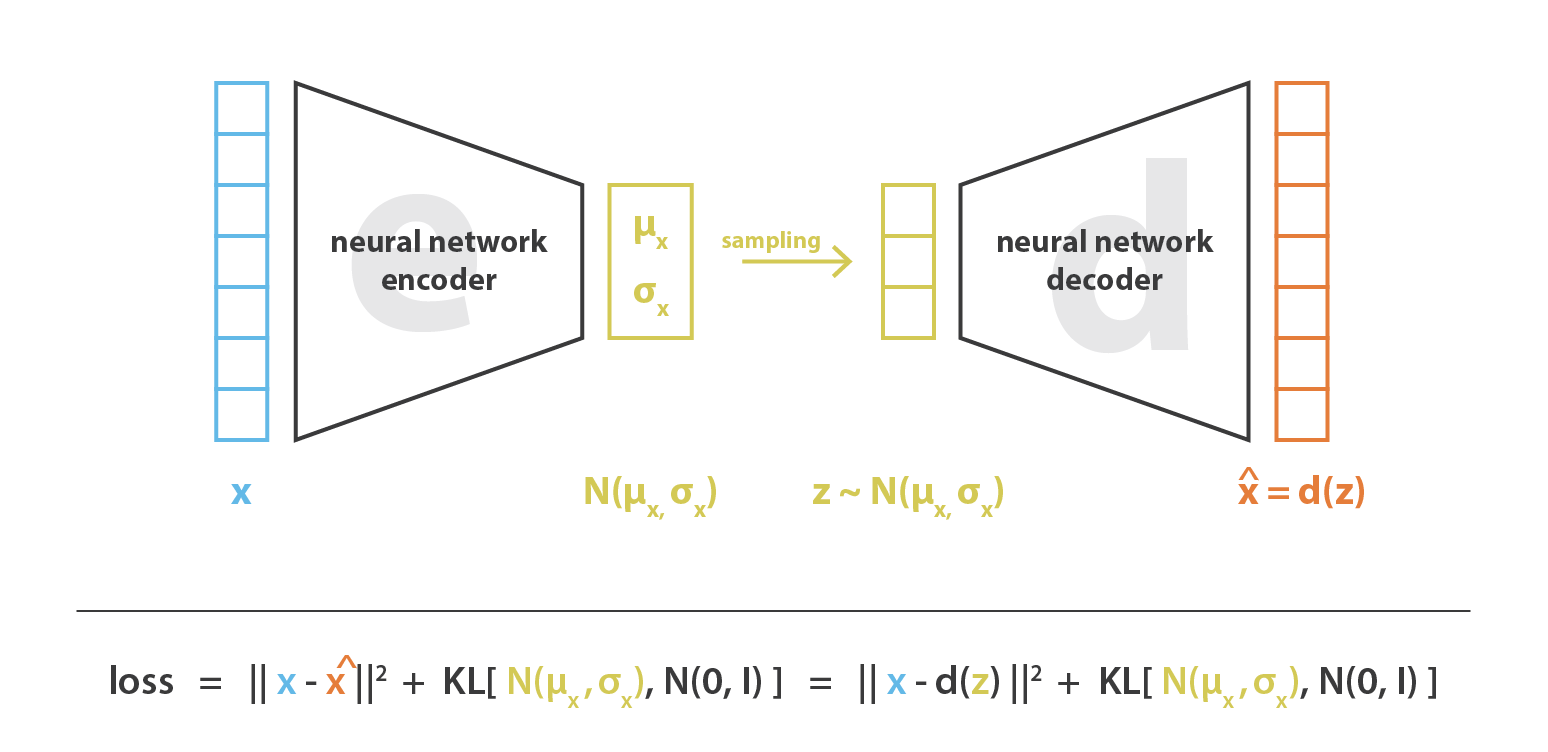 |
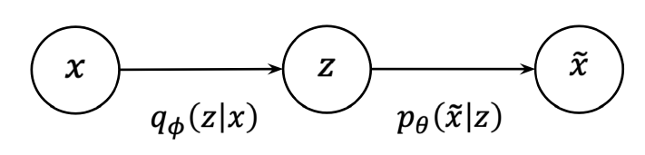 |
where:
-
$KL(q(z)\vert \vert p(z))$ would correspond to the encoder, because we are trying to find out $q(z)$ that is close to $p(z)$
- represents encoding data from $x$ to latent variable $z$
- hence, if going well, this means that the explanation of the data ($z \sim q(z)$) does not deviate from the prior beliefs $p(z)$ and is called the regularization term
-
$\mathbb{E}_{z \sim q(z)}[\log p(x\vert z)]$ would correspond to decoder
- given some sampled $z \sim q(z)$, this is the log-likelihood of the observed data $x$ (i.e. $x_i := x$).
- Therefore, this measures how well the samples from $q(z)$ explain the data $x$, which can be seen as the reconstruction error to get $x$ back from an encoded latent variable $z$
Then the total task becomes learning $\theta, \phi$ by maximizing ELBO:
\[\begin{align*} \mathcal{L} &= \int q(z)\log \frac{p(z,x)}{q(z)}dz \\ &= \int q(z)\log p(x|z) dz - \int q(z) \log \frac{p(z)}{q(z)}dz\\ &= \mathbb{E}_{z \sim q(z)}[\log p(x|z)] - KL(q(z)||p(z)) \end{align*}\]Generation with GAN
The basic idea is that you again, learn some mapping from $z \to x$ by $G(z)\approx x \sim p(x)$. However, do it in the following way
| Generator | Full Network |
|---|---|
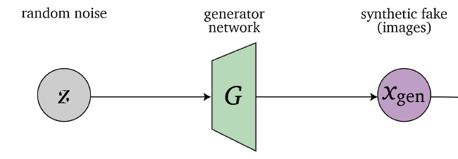 |
 |
where $G(z)$ again learns a mapping, but we train this by the architecture on the right, so that the entire forward pipeline looks like:
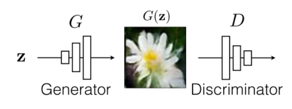
- A generator tries to learn the mapping from prior $p(z)$, e.g. a Gaussian, to the image distributions
- A discriminator tries to provide feedback on how close $G(z)$ is to real sample $x$ it learnt
- then, if the discriminator $D$ learnt some feature (e.g. human have 2 eyes) and used this to tell $G(z)$ is fake, it can backpropagate this information to $G$ so that $G$ can update and learn about the distribution $x \sim p(x)$
So formally we want:
-
generator fool discriminator to say $D(G(z)) \to 1$ being real
\[\min_G \mathbb{E}_{z \sim p_{z}(z)}[\log (1-D(G(z))]\] -
discriminator being able to tell the difference and learn from $p_{data}$ so that $D(x)\to 1$ and $D(G(z)) \to 0$
\[\max_D\mathbb{E}_{x \sim p_{data}(x)}[\log D(x)]+\mathbb{E}_{z \sim p_{z}(z)}[\log (1-D(G(z)))]\]
Together, the loss for the whole network is therefore
\[\min_G\max_DV(D,G)=\mathbb{E}_{x \sim p_{data}(x)}[\log D(x)]+\mathbb{E}_{z \sim p_{z}(z)}[\log (1-D(G(z)))]\]where this is if $D(x)=1$ telling that it is real is a good thing. If you want $D(x)=1$ meaning $x$ is fake, then you would swapped to have
\[\min_G\max_DV(D,G)=\mathbb{E}_{x \sim p_{data}(x)}[\log D(G(z))]+\mathbb{E}_{z \sim p_{z}(z)}[\log (1-D(x))]\]which is a minimax optimization.
Common observation during training:
- at the start, you would initialize $D$ with random weights and its would have 0.5 performance. And $G$ would initially generates random noise
- then $D$ realize you have random noise, hence can discriminate. But this provides a gradient/signal to $G$
- in other words, whatever rule $D$ learnt can be undone/backpropagated to $G$!
- e.g. $G$ generates person with 3 eyes, $D$ realize and learns how to count number of eyes in real images (2), and then $G$ realizes and updates.
- then, $G$ fix that bug, and $D$ will need to learn a new features/rule from the $x \sim p(x)$ that could discriminate.
Note that if $D$ is really good (e.g. pretrained on large task), then it might not work to train a $G$. This is because:
- since $D$ needs to produce a probability, typically we have as a sigmoid behind it
- then, if $D$ is really good, it will always output values very close to $0,1$ as it is very confident.
- But this means that the gradient will vanish as gradients near the tails of sigmoid are minimal.
Therefore, the above architecture/training only work if we have $D$ developing knowledge along with $G$.
Samples from BigGAN
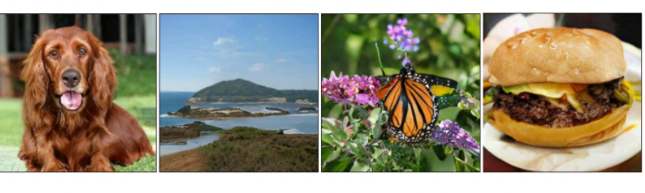
Mode Collapse
Common practical problems with training GANs include Mode Collapse and Convergence issues. Here we discuss mode collapse.
Recall that we wanted
-
generator fool discriminator to say $D(G(z)) \to 1$ being real
\[\min_G \mathbb{E}_{z \sim p_{z}(z)}[\log (1-D(G(z))]\] -
discriminator being able to tell the difference and learn from $p_{data}$ so that $D(x)\to 1$ and $D(G(z)) \to 0$
\[\max_D\mathbb{E}_{x \sim p_{data}(x)}[\log D(x)]+\mathbb{E}_{z \sim p_{z}(z)}[\log (1-D(G(z)))]\]
But suppose $G(z)$ can generated a subset of $x$ being realistic. So that it learnt
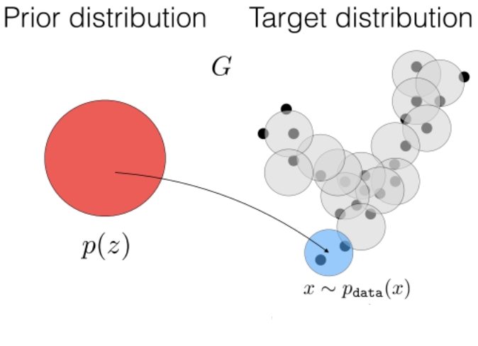
e.g. suppose $p(x)$ are pictures of animals, but if $G$ generates cats that $D$ cannot tell, then it has no motivation to learn another mode
-
i.e. there is no guarantee that the mapping covers the entire image space
-
in theory, this should not happen because if $G$ only learns a subspace of the real images, then $D$ could be able to learn by memory the small set of images $G(z)$ returned, and hence get out of the pitfall. However, it still does happen and it is under active research.
Cycle GAN
The idea of CycleGAN is to do style/domain/etc transfer between two classes using a GAN network:
| Object 1 Domain $X$ | Object 1 Domain $Y$ |
|---|---|
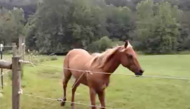 |
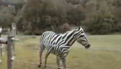 |
where essentially you want to learn:
- a mapping from $X \to Y$
- a mapping from $Y \to X$
So then you can consider having model being
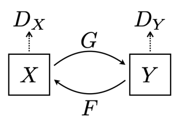
where you want:
-
$G$ learns a mapping from $G(X) \to Y$
- $F$ learns a mapping from $F(Y) \to X$
- $D_X$ discriminates between real $X$ and $F(Y)$
- $D_Y$ discriminates between real $Y$ and $F(X)$
Then naively you might write down:
\[\mathcal{L}=\mathcal{L}_{\text{GAN}}(G,D_Y) + \mathcal{L}_{\text{GAN}}(F,D_X)\]where
\[\mathcal{L}_{\text{GAN}}(F,D_X) =\mathbb{E}_{x \sim p_{data}(x)}[\log D_X(x)]+\mathbb{E}_{y \sim p_{data}(y)}[\log (1-D_X(F(y)))]\\ \mathcal{L}_{\text{GAN}}(G,D_Y) =\mathbb{E}_{y \sim p_{data}(y)}[\log D_Y(y)]+\mathbb{E}_{x \sim p_{data}(x)}[\log (1-D_Y(G(x)))]\]being the losses for normal GANs. However, this would not work as, for example, it does not require $G(x),x$ to be the same object, i.e. it only needs to learn realistic $F(y),G(x)$, but it could be of entire unrelated objects from $y,x$.
Therefore, the solution is to enforce cycle consistency to ensure the transfer is done on the same object
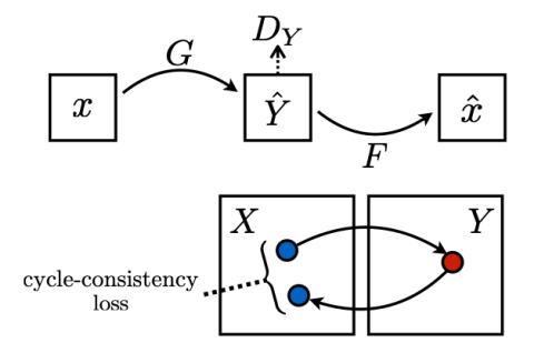
so that you have
\[\mathcal{L}_{\text{cycle}} = \mathbb{E}_{x \sim p_{data}(x)}[||F(G(x))-x||_1] + \mathbb{E}_{y \sim p_{data}(y)}[||G(F(y))-y||_1]\]so that the final objective is
\[\mathcal{L}=\mathcal{L}_{\text{GAN}}(G,D_Y) + \mathcal{L}_{\text{GAN}}(F,D_X) + \mathcal{L}_{\text{cycle}}(G,F)\]Then for training, you would need to prepare paired $X,Y$ ready for transfer
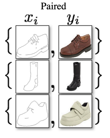
and the trained network could be used for style transfers on test/new images
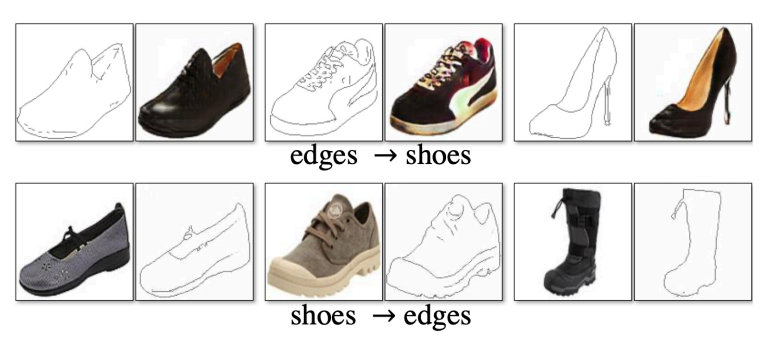
Ethics and Bias
This section will cover a series of real life scenarios where we caused problem due engineers not paying attention to bias/ethics
Note that a lot of the ideas/interpretations written in this section will be subjective.
Unconscious Understanding
It can be said that often those bias/ethical issues crawls in because we didn’t realize that it could be a problem. We often think we understand something, but in reality we might not.
Consider the question of understanding how we see. In the past, people believed that vision is accomplished by emitting beams from eyeballs:
| Past Theory | |
|---|---|
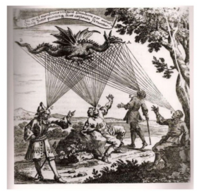 |
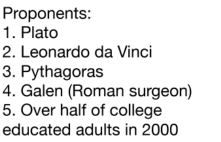 |
But they had some interesting evidences to back up:
- In near darkness, cat eyes are still visible, deer in headlights, also red eye
- e.g. in cartoon, you only see people’s eyes but not there body!
- Taping the eye causes short flashes (don’t try it)
- Evil eye, feel when somebody is looking at you
- how did you feel that? in the emission theory it seems to make sense
- Elegance: similar to touch
But today, with careful experimenting we found that:
- in reality, your retina is just very reflective even of minimal light. (and people in the past cannot make full darkness anyway)
- its blood
- in reality a study is done that people only had $50.001\%$ of the time being able to tell
The upshot is that bias/ethical issues could crawl in in things you believed was right!
Racism with Motion Tracking
In reality, we have a lot of examples with products having ethical and bias issues:
-
2008 HP webcam cannot track black people but white (engineers explained as the training set had only white people)
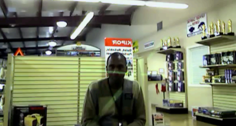
-
cameras tries to make your face “whiter” when auto-enhance is enabled (with the aim of making your photo looks good). But again it is racist!
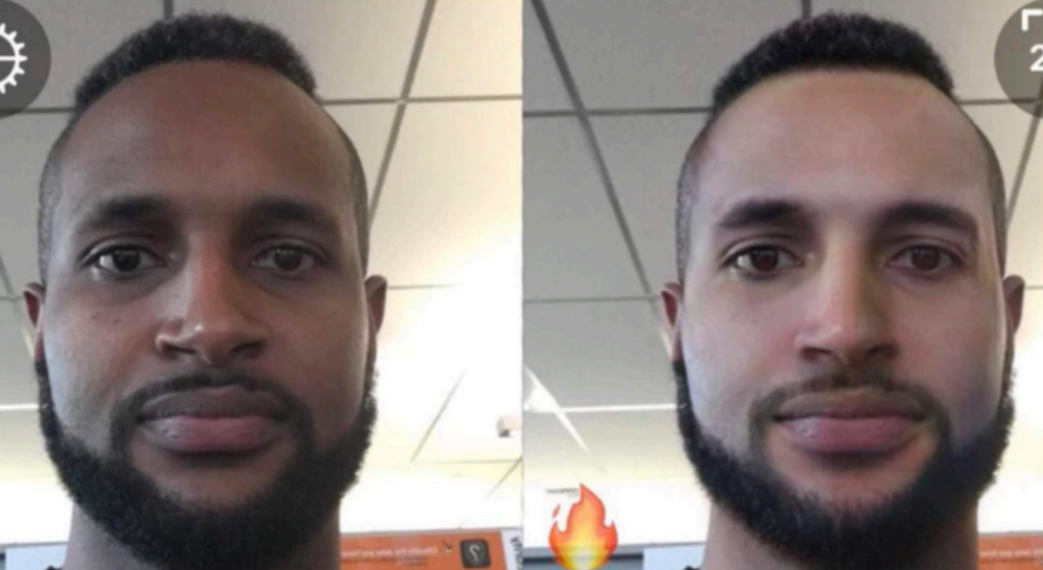
-
ML encoding definition of beauty, which is completely biased!
Is the source of the bias/ethics problem the training data?
Film and Beauty Cards
The below story will show you how some bias/ethical issue can be embedded in everyday objects/tools we used!
Consider how films in the past works.
-
For a black and white film: photons comes through lens and hits the film (which looks like a sandwhich)
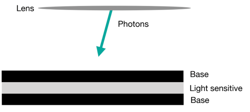
basically depending on the intensity of light, the light sensitive material in the middle picks up.
Then, for black and white files, Film development wipes away undeveloped silver halides, resulting in the negative
-
However, for color films, you have:
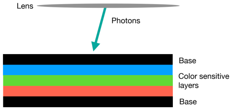
e.g. anything that is not blue nor green pass all the way to red.
Then, when you ship this to the lab, we need to take the channels, find a way to mix them, and resemble them into a colored photo. This means you need to a come up with a chemical process to mix those back. But what is the standard for a good mix?
How do you reassemble a photo that makes you happy?
Film companies distributed reference cards so labs could test their color reproduction.
Then this gives the first Shirley Card:
| First Shirley Card | Other Shirley Card |
|---|---|
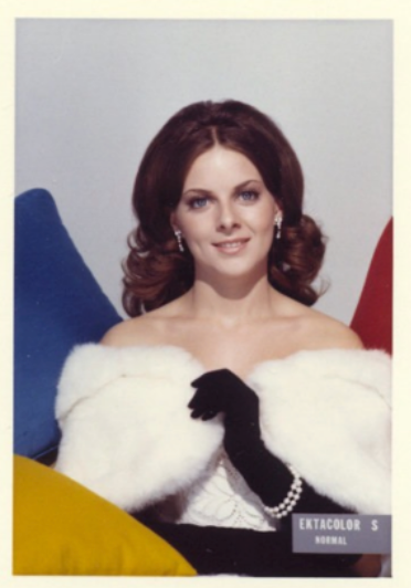 |
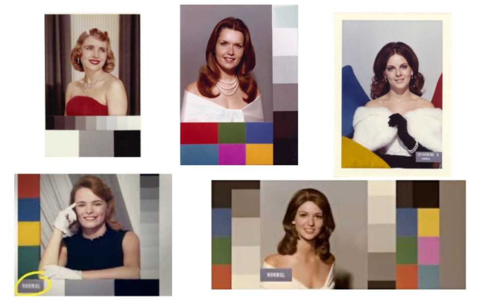 |
so that people calibrates machines/color mixings according to those cards. Apparently we see the definition of beauty in colored photos is bias towards white!
As a result, if you take a colored photo of the blacks at that time:
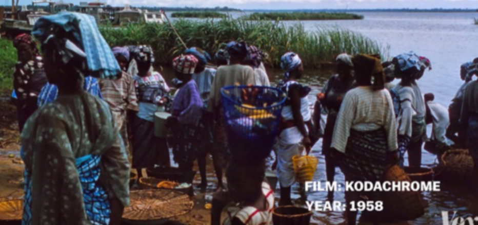
so that the exposure is so bad that yuo cannot see the facial details of those black people.
What is the solution? We should fix the training data to include diversity:
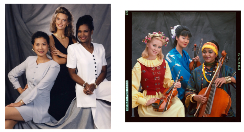
(but what actually caused the change are advertisings, e.g. chocolate does not look good, not due to complaints from people)
However, the source of the problem are people themselves.
- whatever reference set we defined is subjective, which is in the end defined by people
- it is sometimes all those tiny decisions you (carelessly) make that propagates to the society and becomes a bias!
Many other examples show-casing how people themselves produces bias include training models based off internet:
- learns to tag black people as terrorists, because there are patterns/statistics that does have this correlation
- Tay chatbot on twitter
Image Processing and Lena
Early reference image used in image processing commonly included the following image:
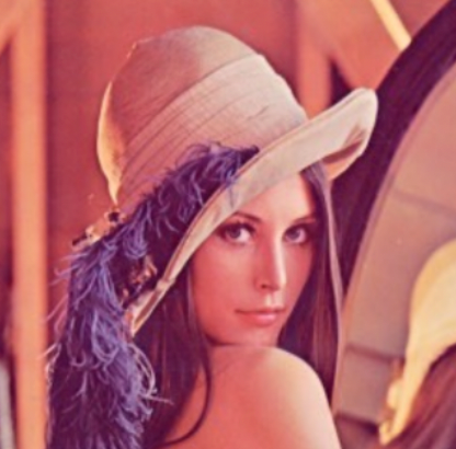
where for image processing, examples include:
-
find a compression technique such that this photo looks good.
-
etc.
But why this picture? Do you know where it comes from when you are using it?
- this image is a crop from a photo originally in an adult magazine (Playboy)
even today, we compare results, papers on this picture!
- again, these tiny. careless decisions people make could have impact! (those temporary decisions could be stuck in the entire industry)
- but people would just use those biased dataset, for example, without realizing that this could be biased. However, the motivation would sound justified: we do not want privacy issues, hence we end up using those public images which are usually celebrities
And the only way to break it is to have people along the line of using it to be aware of every decisions that you make.
Tay Chatbot
Consider producing a bot that maximizes likes on twitter
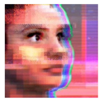
Then after 16 hours of deployment, this chatbot
- Learned to retweet offensive messages
- then was shut down
Again, problem is the training data. Yet who creates the training data? It is us ourselves!
Facial Bias
In the past and even today, you might hear:
“Facial recognition is Accurate, if you’re a white guy”
In 2018, some results show that commercial facial recognition on gender identification when given a photo:
- white man has 1 percent of error
- black man has up to 12 percent of error
- white woman has 7 percent of error
- black woman has 35 percent of error
“One widely used facial-recognition data set was estimated to be more than 75 percent male and more than 80 percent white, according to another research study.”
And you also have a lot of bugs as well in the system:
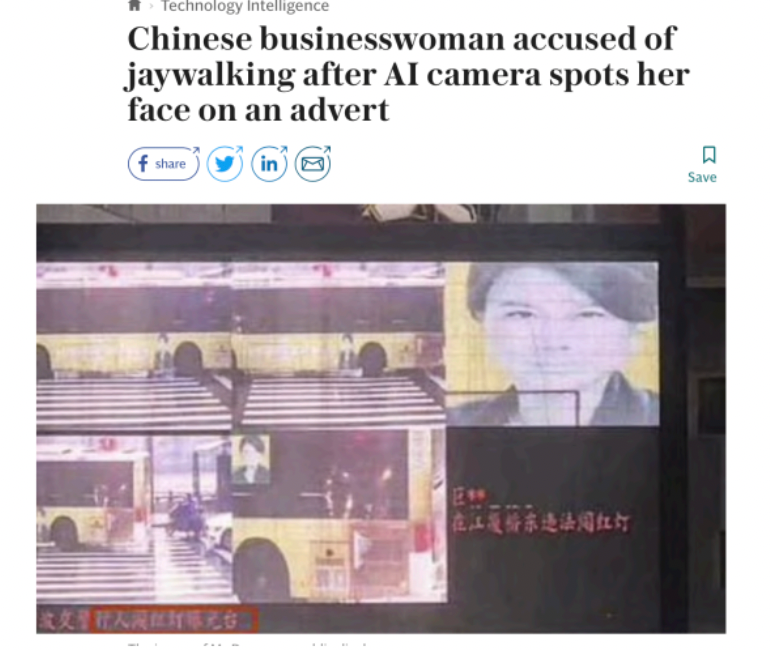
which are all examples where you think vision is easy but how do you build a system that avoids that error.
Criminality and Sexual Orientation
Some very controversial research were even published on the topic of:
-
Given a face, inference the likelihood of crime.
- https://arxiv.org/abs/1611.04135
-
Attempting to predict sexual orientation from facial photograph
-
first we need to collect dataset. One way they did is to download photographs from a dating website (another problem of data privacy)
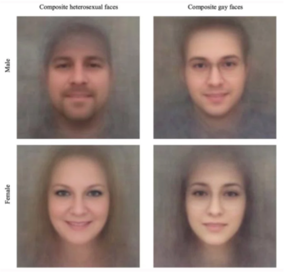
where the first column would be heterosexual, the second being homosexual.
-
Found some correlation, and claimed it was due to facial structure (i.e. had a non-chance performance)
However, in reality
- there is a superficial bias that is hidden, such as angle of taking a photograph, whether if there are makeups or wore glasses, etc.
- so if you control on those variables, the performance becomes pure chance.
-
Again, many work comes from good desire but the approach is pure fallacy if you do not take care of bias/ethics
Career-wise advice: join a diverse team! We engineers have to start insisting on preventing those biases.
Fairness and ML
fairmlbook.org
Vision and Sound
In a video, we not only have the visuals, but also the sound! In general, we have many multimodal data in reality to deal with
When dealing with those data, keep in mind that there are rich interaction between modalities
A famous example will be the McGurk effect
where even if the audio is the same:
- if the mouth movement changed, you might hear “Ba” or “Fa”
- when you have conflicting data in modalities, how does your mind resolve/combine those information? which one is your brain listen to?
- If you have conflicting perception, you will trust your eyes. (one possible explanation is because your vision system works faster)
But most of the time, normal/natural data will have correspondence between modalities. In this chapter, we aims to build models that exploit those interactions.
- an example application would be to train a model that can locate the source of a sound (e.g. an instrument) from a video
- denoising algorithms (has nothing to do with vision)
Human Ear
Before we look at how to build systems on solving the above mentioned problems, first we can look at how human ear works
Essentially how we hear is by having sound waves hitting your ear drum, so that
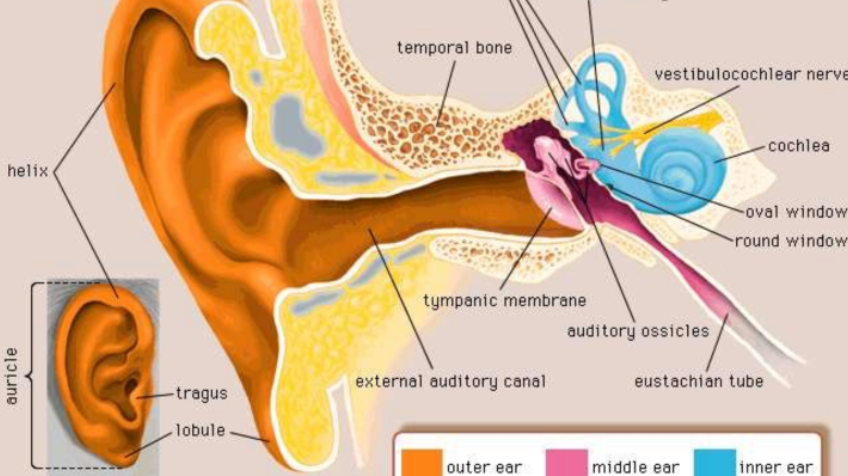
-
vibration of air causes some bones in your eardrum to vibrate as well
-
then the vibration transfers to cochlea: which essentially does a “FT” (vibration in fluid) by activating on different frequencies
- when you get old, some parts of your cochlea breaks down and you cannot hear high frequency sounds
Additionally, if you loses your sight, the system that processes your vision will switch to hearing, so that
approximately all the vision related regions in brain will adapt to hearings, hence:
-
you end up having acute hearing
-
the adaptation happens in about 6 month
An interesting experiment would be that, if you spend times with only touching/hearing things, but then given sight back, can you recognize the same object you touched?
Sound in Computer
Now, to deal with sound information, first we have to know how to represent sound into “numbers”.
How do we represent sound in computer?
Computer represents sound by resenting its wave: by variation of amplitude (air pressure) over time. But more often we do a FT of the waveform to get a frequency domain: spectrogram/sonographs
| Amplitude | Frequency |
|---|---|
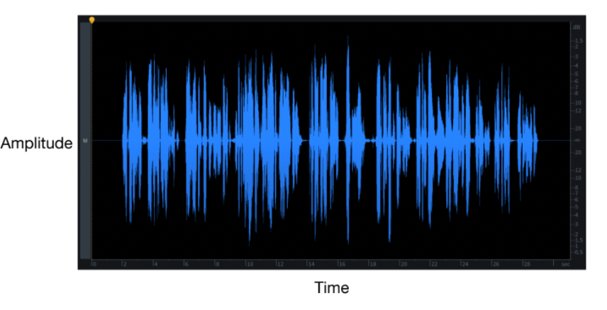 |
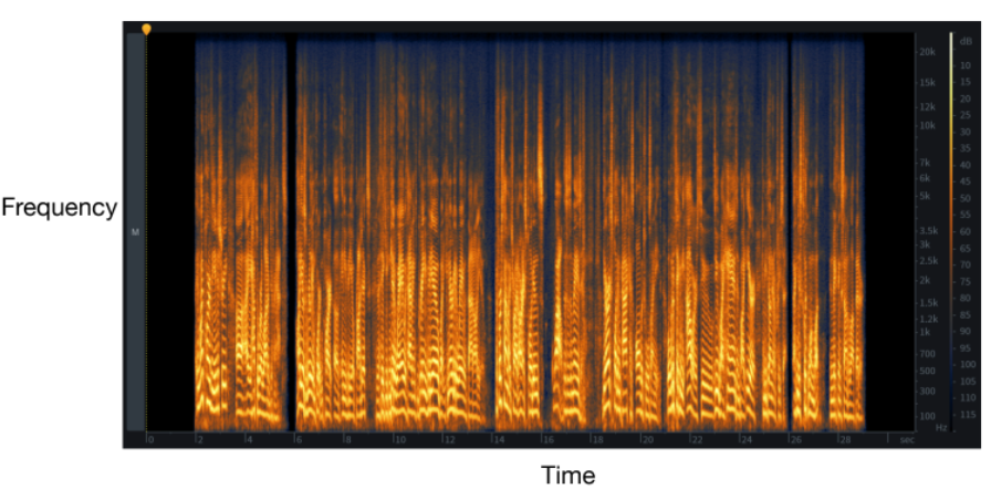 |
which is basically doing two things: a) break the amplitude-time graph into several windows/partitions; b) for each partition get a Fourier transform $G(f)\to (A,\phi)$ for the wave inside that partition; c) concatenate them back with time where now the color/brightness represents the amplitude
-
recall that a fourier transform of a Amplitude-Time graph gives Frequency-Amplitude:
Wave within a Window FT 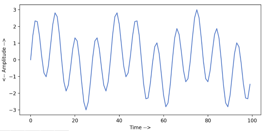
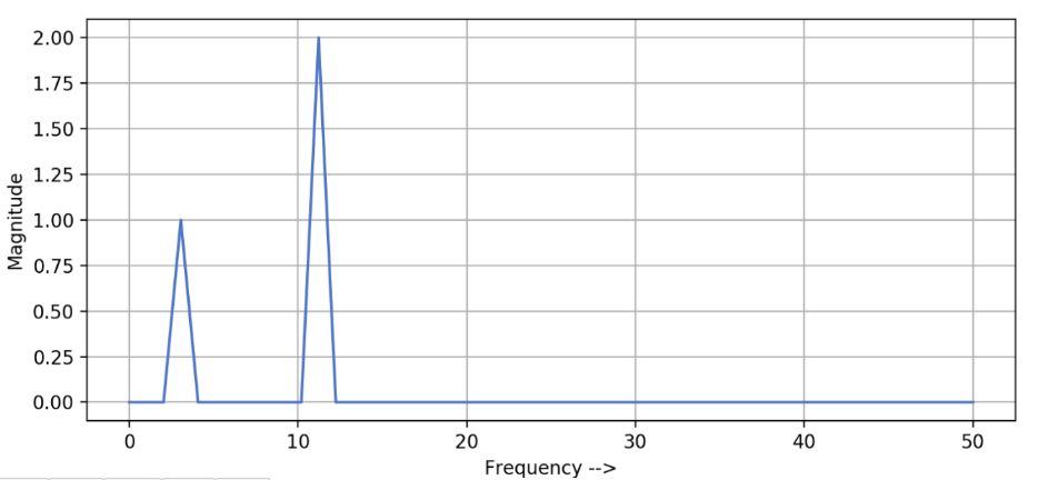
note that with only a FT, you lose the time information/ordering (which is an important feature if you want to use this as input to a model). This is why we have spectrogram as a representation.
-
in the example example, we see that at time $t=0$, we have few high frequencies, but many low frequencies. Therefore, we also get only a few high frequency waves (i.e. many have $A=0$ for high $f$, less dense/bright on the right figure) but dense low frequency waves.
-
for humans, we can only hear up to 22,000 hertz. So if it gets high frequency regions in the chart, we might not be able to hear it.
Some more examples include:
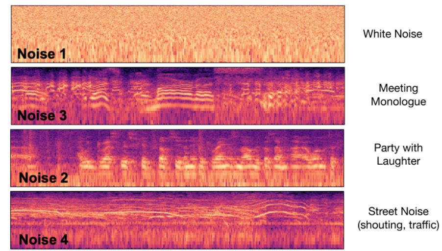
where notice that:
- white noise has a “uniform distribution”: all frequencies everywhere hence the brightness/density is approximately the same.
- for party with laughter, we see many high frequencies data present as compared to the other ones
- this also means that if your hardware ended up adding/manipulating the spectrogram, then you will hear a slightly different sound
Learning to Hear
Essentially all techniques mentioned in video works in audio.
Our aim is to:
given a spectrogram $x_s(w)$, i.e. sound data
learn some task-related information from it (e.g. what object does it correspond to)
\[f_\theta(x_s(\omega)) \to \text{objects}\]or you can learn other things such as the location of the image that produced the sound
Many architecture for sound, which is essentially 2D data, can be basically made similar to a ImageNet (note that the only difference is that you would expect sound data to have a high width-dimension as you typically have a high sampling rate for sound)
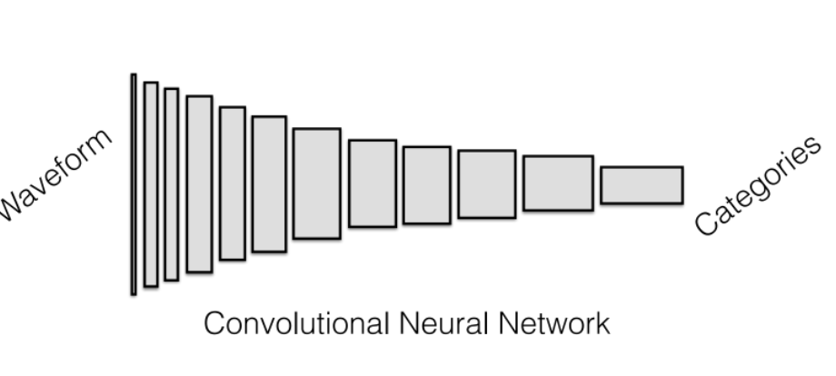
most of the hard stuff is how do we get training data (for free). Usually this is done by utilizing the synchronization of videos which have both a sound and vision perspective.
Then consider the task of associating an object from a given sound
| Input Sound (of a Lion) | Output |
|---|---|
 |
Lion |
We can Use natural synchronization of sound and video to “label” the sounds. We consider that, from a video:
- use a network $F$ that learn the objects and scenes in the picture $F(x_v)$. Use this as a teacher
-
use a network $f$ that deals with sound input $f(x_s)$. This will be a student
- use KL divergence to match the distribution between by and student model
Hence this is basically what SoundNet does:
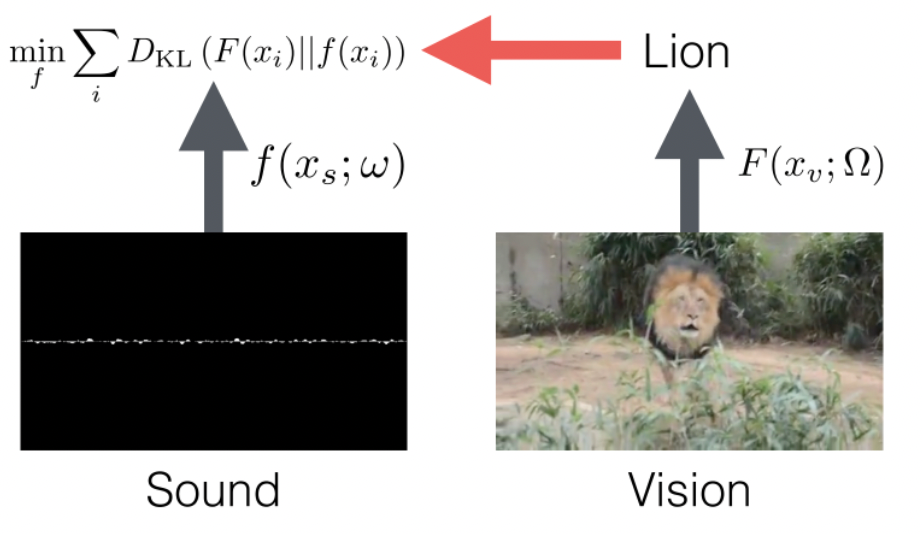
then it learns that, given a sound, what are the objects and scenes in the sounds:
-
we usually first train the model $F$ alone (or take a pretrained model), so that it is treated as the teacher
-
then, the student network $f$ tries to learn a mapping from its own data to the output of the teacher network
-
as a result, it can learn that the above particular sound should correlate with the object of lion
However, there are “problem” cases. Consider the example of
| Example Input: Dog barking | Example Input: Birthday |
|---|---|
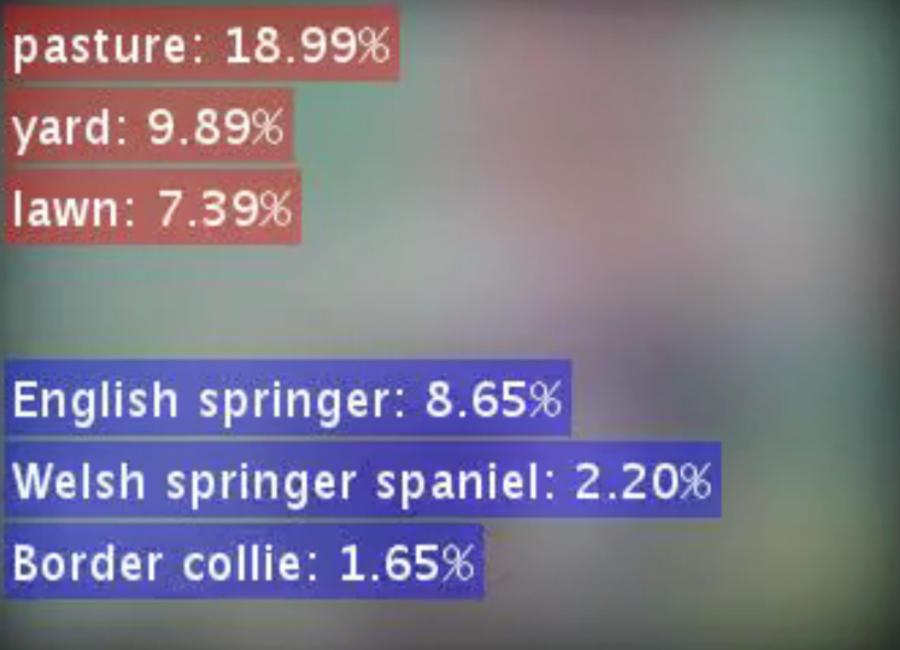 |
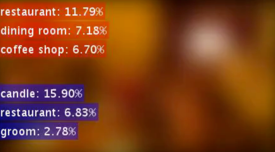 |
notice that both cases above where output of $f(x_s)$ when only given sound
- on the left figure, it even found the breed of the dog (extra information learnt due to the vision mapping)
- on the left figure, can also tell some background sceneries, e.g. on a pasture. (extra information learnt due to the vision mapping)
- on the right figure, it predicts that there are candles when only given a sound of happy birthday (extra information learnt due to vision mapping)
- technically the above are forms of “spurious correlation”. But whether if it is good or bad depends.
Finally, for completeness, below is performance of SoundNet for classification:
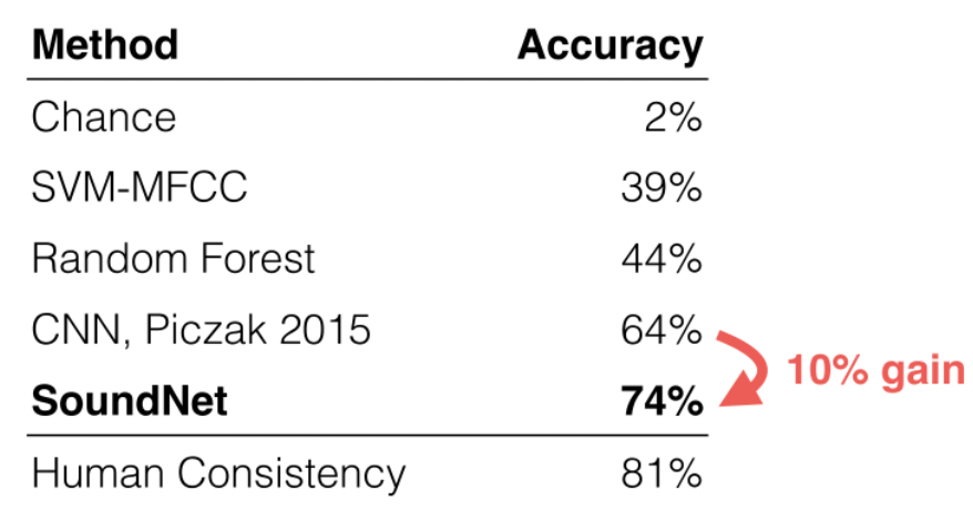
Cocktail Party Problem
The cocktail party effect is the phenomenon of the brain’s ability to focus one’s auditory attention on a particular stimulus while filtering out a range of other stimuli.
With this ability we can easily/fast switch attention to people mentioning your names in the noisy background
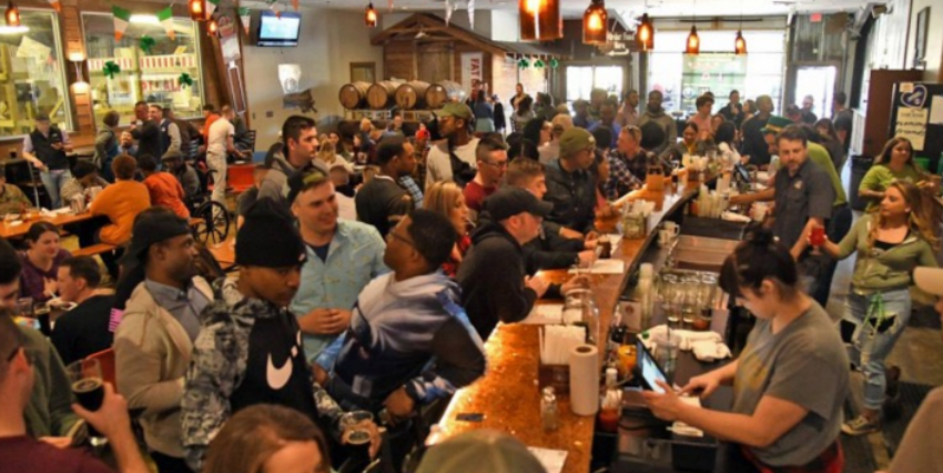
A related task in DL would be:
Given a sound/spectrogram that is a composition of sounds (e.g. two musicians playing), can we build a network so that we can choose to attend to one player’s sound while filtering out the other?
- essentially the problem of unmixing sounds
The aim would be to build a program so that:
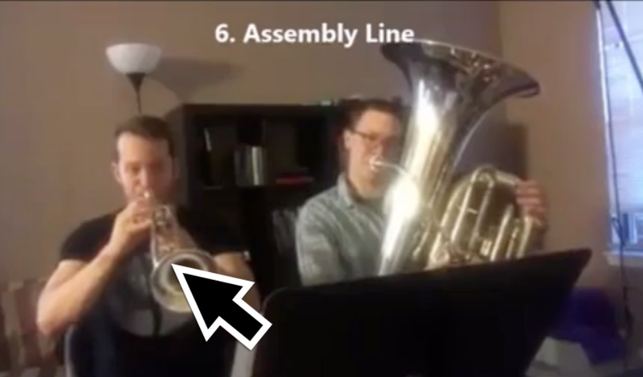
if you click on a person/instrument, you will attend to a specific person/instrument’s sound (i.e. only hear its sound)
To make the above application, we need a network that figure out which regions of the video are making which sounds.
- the final hidden aim is to unmix the sound in the video
So essentially:
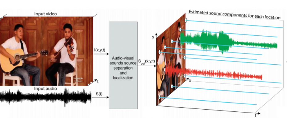
but again how do we even get training data?
- Again the trick is to utilize the fact that videos have synchronized audio and vision information
- sppose we have $N$ videos with a single player producing some sound. Then we can compose $2^N$ video by:
- choose a combination of the videos (with their sounds)
- concatenate the video and add the sound (assume each mixed sounds are sums of spectrograms)
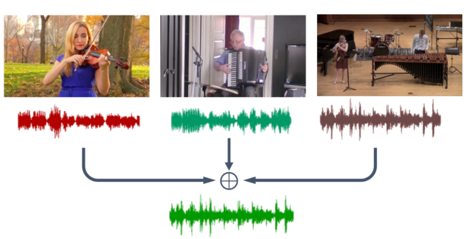
Then we automatically have labelled data. But recall that we need our network to do two things:
- unmix the audio
- assign which region in the video each unmixed audio comes from
The biggest problem is that there are infinitely many solutions for un-mixing + assigning:
- there are infinitely many ways to unmix the audio
- even after unmixed, how do we let it learn which location it comes from?
To solve this problem, consider formulate the problem to be reconstruction task:
- given a mixed video + audio input
- find some $k$ video embeddings $i_k$ and $k$ audio embeddings $s_k$ (i.e. learning unmixing/separation)
- let the video embedding choose which audio embedding it has (e.g. similarity)
- reconstruct the sound from using those $2k$ embeddings
High level architecture
| General Architecture | Detailed Architecture |
|---|---|
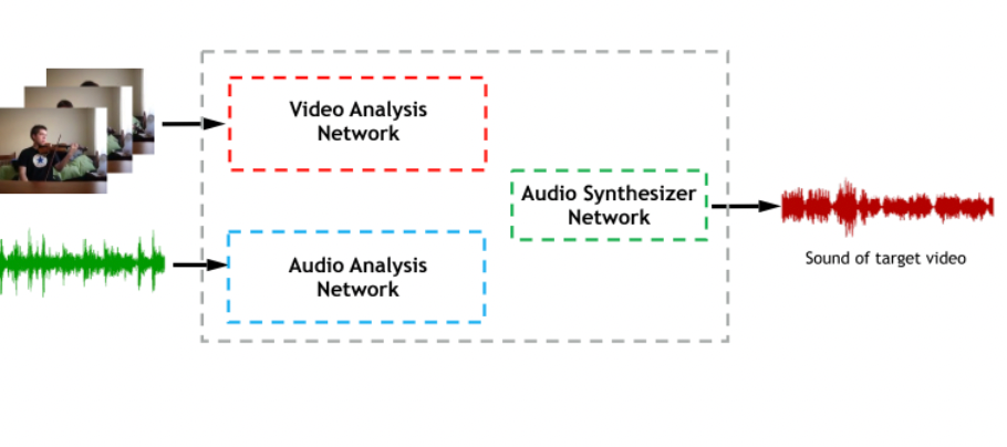 |
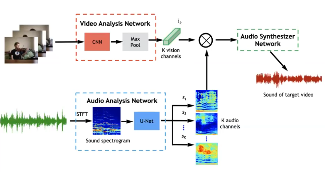 |
so that essentially
- we want the network to get from one spectrogram to $k$ spectrograms
- then the key idea is that the audio NN should learn what are the $k$-channels that can best reconstruct the original sound!
Then if we have large enough data:
- each $s_i$ (e.g sound of a dog) would correspond to the vision of $v_i$
- technically you can choose a $k$ that is large, so that even if there are less objects than $k$, we can have the vision “fragmented” $v_i$ and $s_i$ so that when we “click” on the object, we just sum the fragmented sounds and get back the sound of the object
- so technically it learns by separation by category, so that if you have multiple instances of the same instrument, then it won’t work
Once trained, this system can
-
manipulate volumes of of each individual instrument as now we have it seperated!
-
also create a heat map knowing where the sounds come from
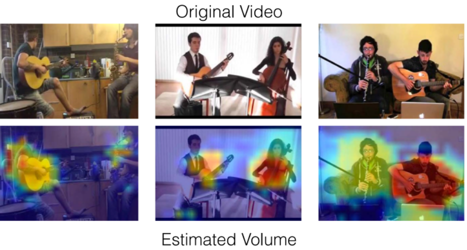
Interpreting SoundNet
We mentioned that the same architecture of CNN can be used for sound. Then what does the kernel learns to do?
For instance, recall that the firs layer in CNN for vision learns to detect edges:
| Layer | Kernel Visualization |
|---|---|
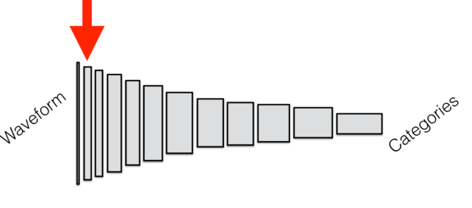 |
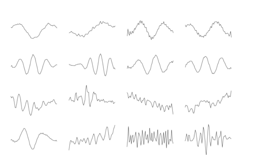 |
it turns out that the kernel for sound at layer one:
- detects low frequencies and high frequencies
- the “edge detectors” parallel for sound
Moving on, for middle layer kernels activates specifically for an “object” of sound. E.g. smacking/chime sound (i.e. only hear those = only those got activated after some neuron)
| Layer | Activation “Map” |
|---|---|
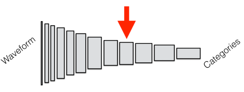 |
 |
Then in an even higher level, there is a unit activates on an even higher level “object” of sound (e.g. one parent talking to kids)
| Layer | Activation “Map” |
|---|---|
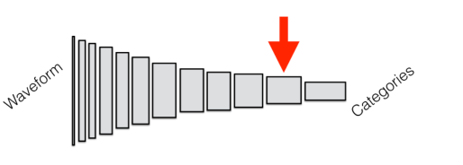 |
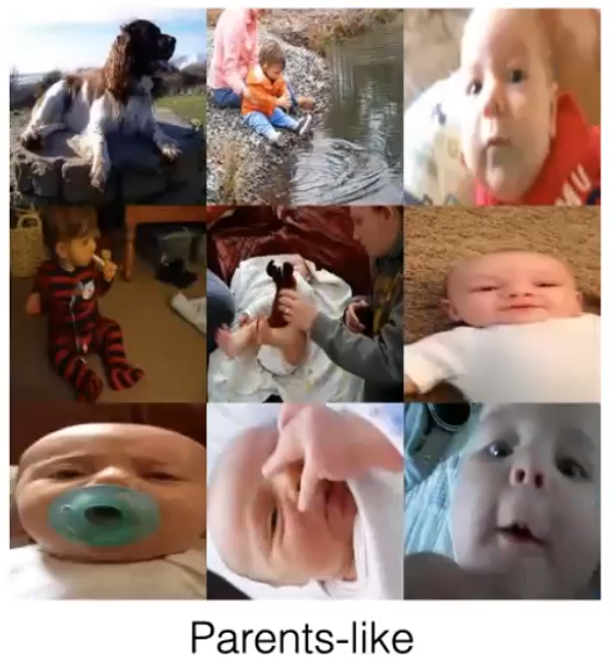 |
Clustering sound
Once we have embeddings of sound data, we can cluster them based on distance (e.g. below uses MDS)
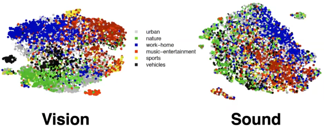
where here we compare how vision and sound data relates to each other
- green/nature cluster: images/vision about nature seems to be close together in “semantics” as they have similar embedding
- yellow/sport cluster: for sound, they are spread all over the space
Additionally for sound data specifically:
- music are being close together, forming a cluster
-
urban and nature seems to be close in sound representation
- clustering becomes more diverse
Denoising
How do we suppress the noise in a video conference call? Solving this task essentially leads to
How do you figure out which part is signal (our speech), and which part is noise? (Hence do noise removal)
- note that this is purely an application of hearings, no vision related techniques are applied
One key observation/property is that human needs to breathe, hence we get silent intervals. Then during those silent intervals, estimate the noise distribution:
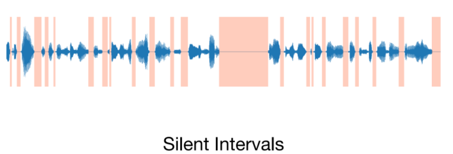
then we want to estimate the noise using those intervals, and then subtract it to get denoised input.
Then the architecture looks like
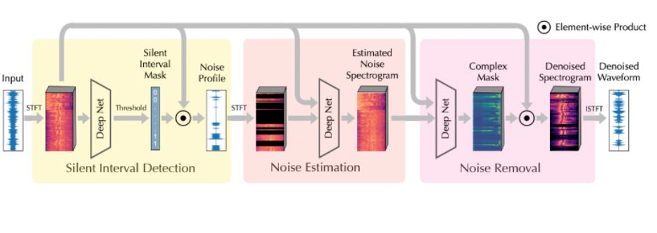
Vision and Language
What is an ideal AI system? Ideally, we would want it to be able to do:
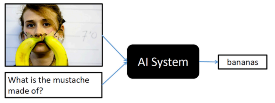
Notice that to answer those, we not only need vision, we also needed NL understanding, as well as:
how to combine two two information/query and data
some common sense (see below)
. More examples:
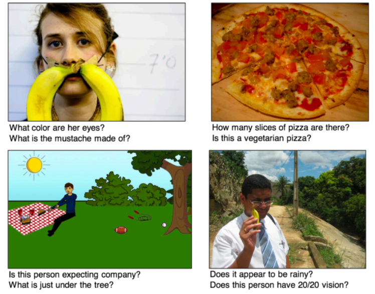
where notice that:
- we need encode the given data which is both in vision and text
- we also need some common sense encoded in the system, so that we can answer the bottom row questions
Trial Architecture
If this solved, then it is real AI! But it is not yet solved, and some simple approaches just brute force combining embeddings of everything:
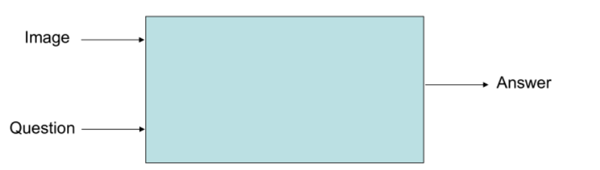
where the question is how do we fill in the black box.
Recall how we can representing Words: One NLP task is to find similar words given a word
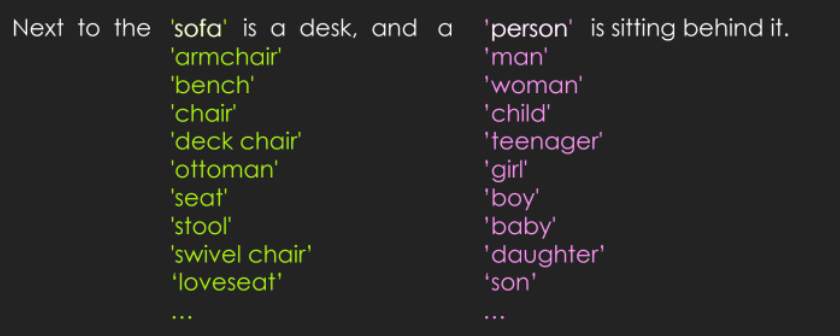
which essentially is to find embeddings given a word and hence produce similarity scores.
- word2vec embedding
- Glove embedding
- BERT
- etc.
Then a sample architecture comes out as
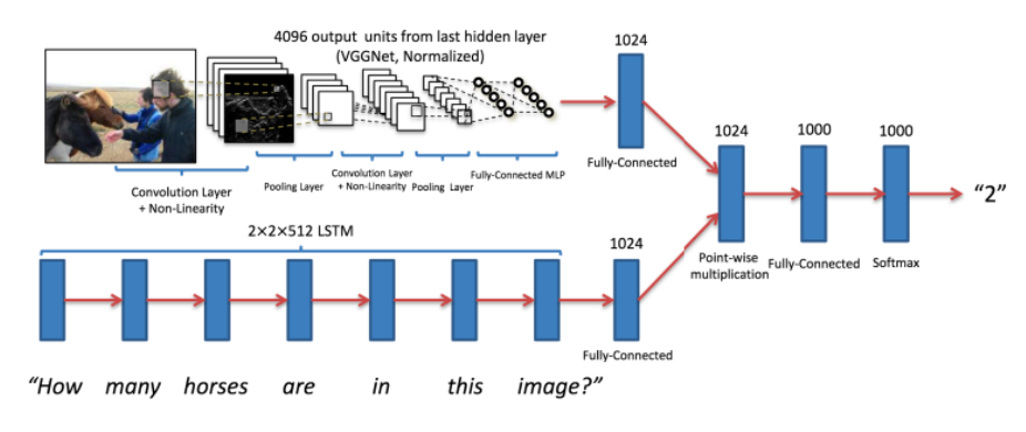
Then if we have enough data, we hope to encode common sense in the system as well:
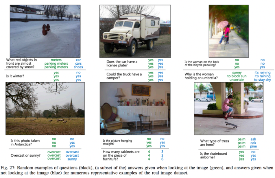
where
- green is when we gave both text and image as input
- blue is when we only have text as input
- notice that there is a great potential of the network just learning by memorization/overfitting
But some times it works. Some applications that comes out from this:
| Examples | Examples |
|---|---|
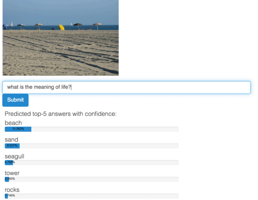 |
 |
however, there are problems:
| Inconsistencies | Inconsistencies |
|---|---|
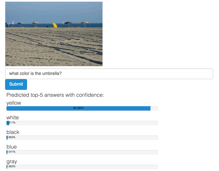 |
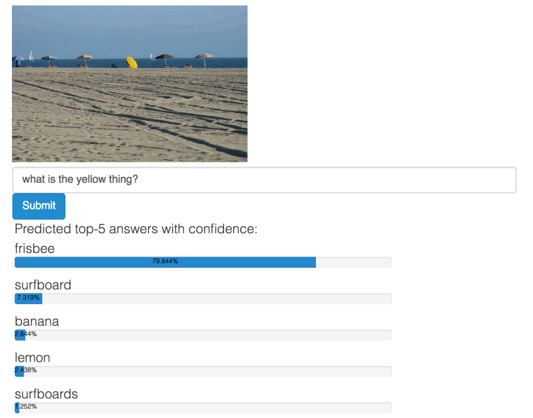 |
where we see that
- there is no self consistency (yellow frisbee)
- it is perhaps not how a person answers the questions (its common sense is not the same as ours)
- overfit, biases comes in, etc.
Compositional VQA
Instead of finding a model to answer the question, let the model learn the logics to reach the answer
- that way, we can perhaps control the bias that would be learnt from the NN
Consider the following questions on the compositions you have in the image:
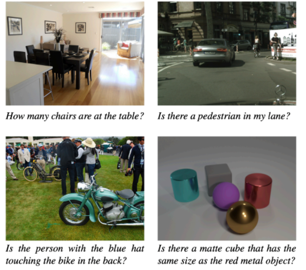
We want a NN to synthesize a program that outputs the answer
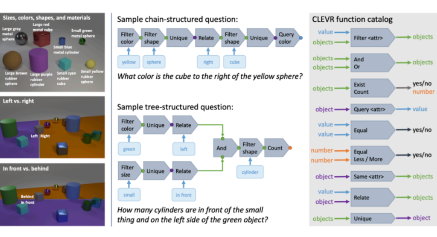
where:
- right column includes the operation you can have for the program to do
- then, the network learns to assemble pieces to output a program
- so that when you run the program, you get answer to the question
Therefore, your architecture looks like
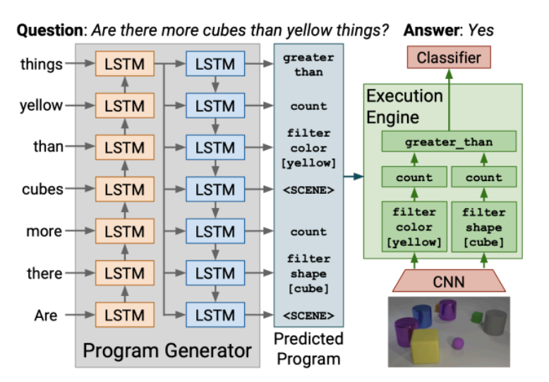
where essentially the
- program generated from the text only, so there might be efficiency issues.
- the objective is to produce the same program given the same question, so that we have predictability (even if we swap the image input)
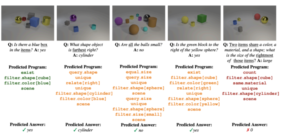
Relational Network
To answer the question, we need to first learn some mapping/correspondence between parts of the image and words in the question. Then answer the question.
Google came up with a this network that solve the following types with 99.9% performance
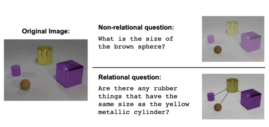
where the big difference from the previous is:
- if one component of the program is wrong, then the performance is bad (i.e. structure assumptions we are making, which works only if right)
- but for black box approaches with NN, the risk is much smaller
The idea is to basically
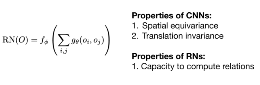
so that we view image as patches of pixels, and sentence as a patches of words
- then each patch of image would correspond to each word/phrase
- $O$ is a set of objects, where an object could be a pathc of image or a word
- basically consider all possible pairs, and produce a feature representing those pairings
Then there is very little assumptions made
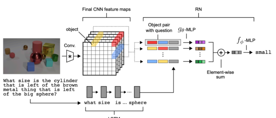
3D Vision
Why you have two eye balls instead of one? It might seem redundant that you have two eyes looking at the same direction = why do we need this extra redundancy? Why did evolution not have our second eye at the back of our head?
It is with such “redundancy” that we can perceive depths.
Binocular stereopsis, or stereo vision, is the ability to derive information about how far away objects are, based solely on the relative positions of the object in the two eyes.
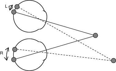
Human Vision and Applications
Many animals also have stereo vision:
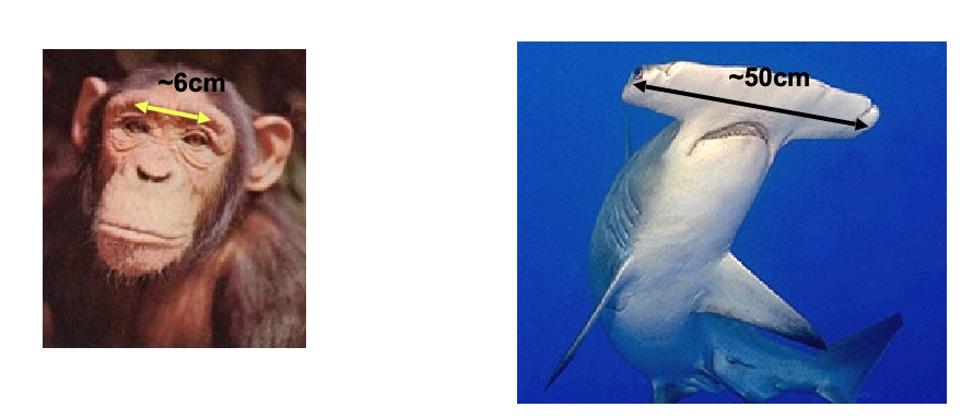
and the further the separation is, the better you are at seeing depth (e.g. for very far away objects)
-
This is very important for predator: how far away are you from the prey?
-
On the other hand, prey sometimes doesn’t need this. For instance. for pigeon, it is more about seeing 360 vision instead of depth
- Therefore their eyes don’t need to “overlap” but goes “sideways”
- however, they still can achieve some stereo vision by moving your head in some particular away
Stereoscopes: in the 19th Century we already had goggles that you can wear to see 3D pictures
| In the past | Today |
|---|---|
 |
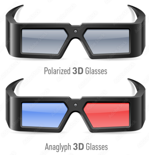 |
but they are typically very expensive.
- today we often have a cheaper way: we construct the visuals in a way that pairs up with the goggles on the right
- it works by having only red light passes through the red lens, and same for blue, to create an illusion of 3D. Essentially it controls which eye sees which view to render the entire scene 3D!
Mars Rovers: Very expensive, so we want our rover not to hit/crash into any obstacles!
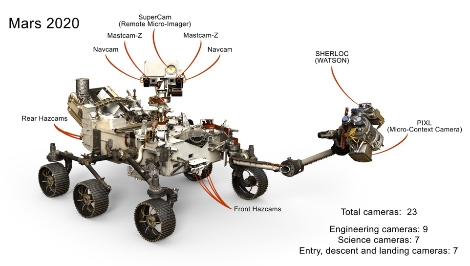
so we see that it used many cameras for stereo vision and hence navigation.
Depth without Objects Recognition
How does your brain merge the two views you see in two eyes to get a 3D perception?
Some interesting experiments done in the past considers whether if we performed object recognition first and then depth:
- e.g. could it be that because I know it is a table, I know the depth? i.e. we know the priors and use for depth perception
- turns out to be not the case! we directly see depth without object recognition, as shown in the experiment below
Random dot stereograms: consider concentrating on the two squares highlghted on the le
| Random Dot Stereograms | Human Perception |
|---|---|
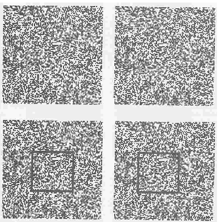 |
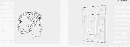 |
the idea is simple:
- take two noises, and take the same two squares in the noise as shown on the left
- if you can cross your eyes to put the two squares on top of each other, it will seem that the square is closer to you than the background
- this shows that depth has nothing to do with objects recognition. You directly perceives depth somehow!
Important of Depth Information
Consider the following examples:
| Left Light Source | Right Light Source |
|---|---|
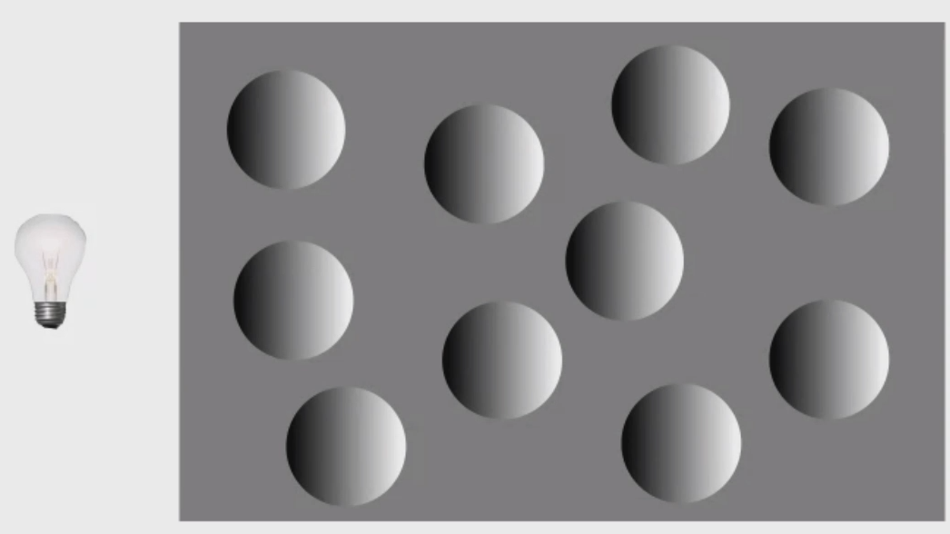 |
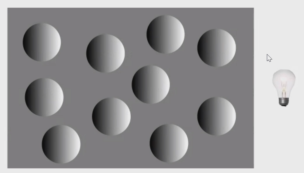 |
where:
- on the left you should perceived that the holes are sticking in, whereas on the right the holes appears to be popping out
- but we have the same image, hence whether if the holes are sticking in/popping out is ambiguous if we don’t know the location of the light source (or resolved if we know the depth!)
Similarly, which vertex of the square is sticking out/which face is in the front is ambiguous:
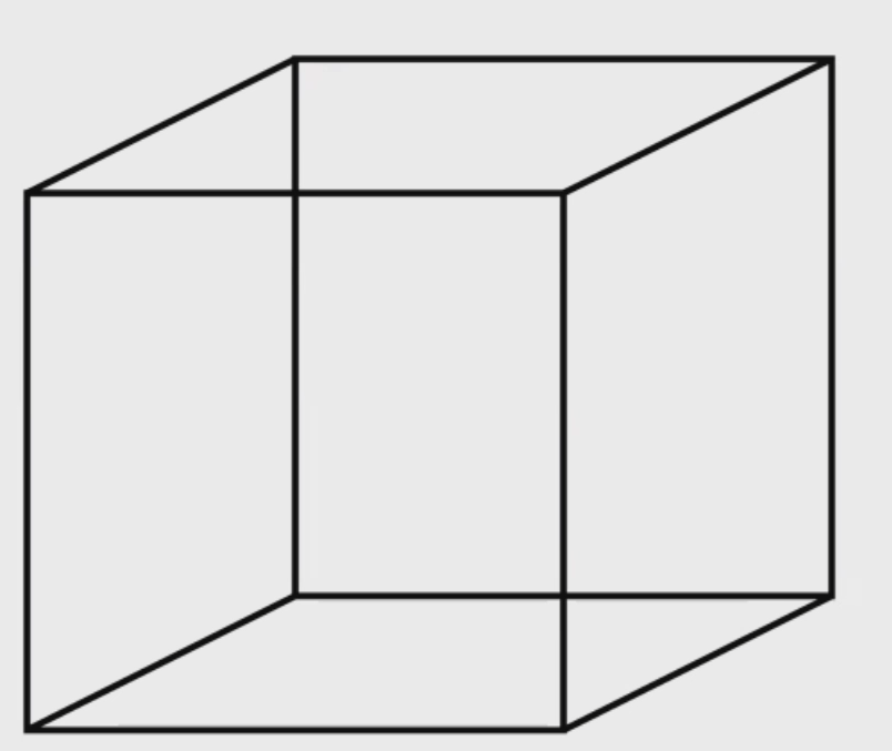
it all comes down to putting a 3D object 2D loses information:
- there can be infinite many 3D configurations that have landed in the same 2D picture shown above
- ambiguous what the original 3D object is without depth information
Perceive Depth with Machines
How do we use algorithms based on geometry to see depth?
- e.g. given an object and some cameras, how do you construct the depth information of the objects?
- once we understand how this works, we can maybe inference some new view points and construct 3D scenes you never saw before!
There are two common approaches to calculate depth (given some view point), and to construct 3D visuals:
| Binocular Stereo | Photometric Stereo |
|---|---|
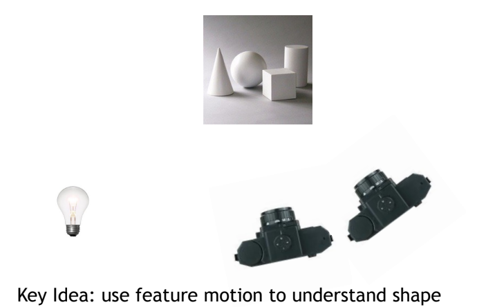 |
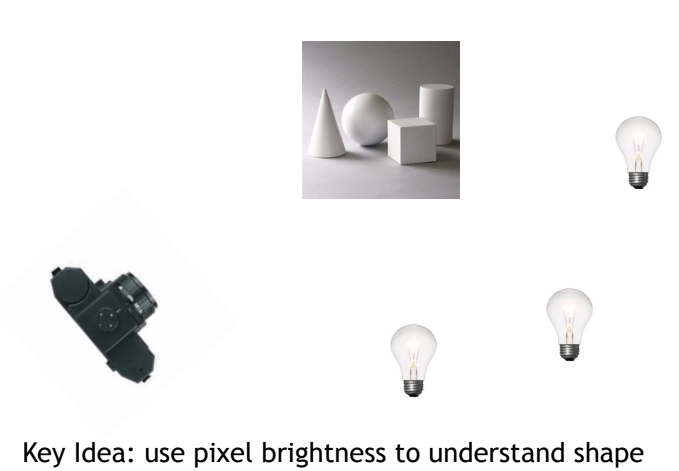 |
where
- Binocular Stereo: like our eyes, we have a second camera
- based on how far away the pixels move when we “move” our camera, we can estimate depth
- i.e. things are far away will have almost no movement when we shifted the camera, however for close objects it will have some movement that is related to how far it is from the camera
- Photometric Stereo: only one camera but lights move around
- essentially computed based on changes in pixel brightness
- actually works very well in practice
If this works well, why do we need ML on this?
For estimating the depth of a point, we need to figure out changes of a pixel when we changed the camera position/light. However, this means that we first need to know which pixel are corresponding to which pixel in the different images we took.
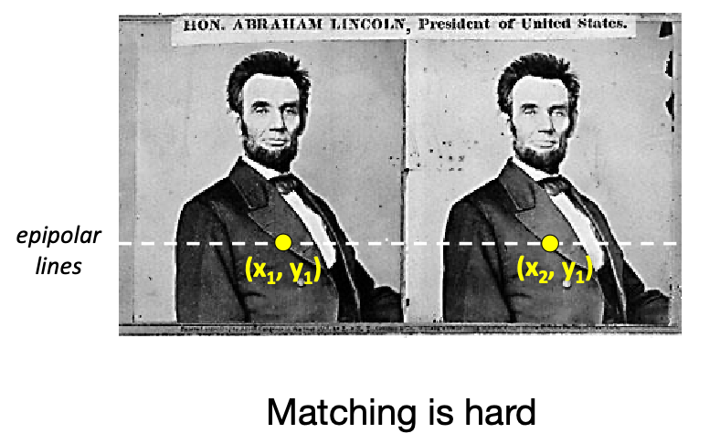
Given two matched pixels, we can of course figure out how far they moved, and therefore depth:
- but how do we find the matching pixels on the first hand?
- then, how far did they move/how many pixels did it move/change?
Applications of Using Depth
More examples using ML to find out depth information could be useful
Necker Cube
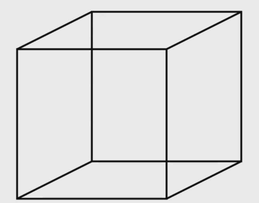
with many data samples of the same cube taken from different angles, we can use ML to estimate depth and hence reconstruct the original 3D object!
Facial Recognition
For face recognition, we need to build a 3D model of your face
| Facial Recognition | Modeling |
|---|---|
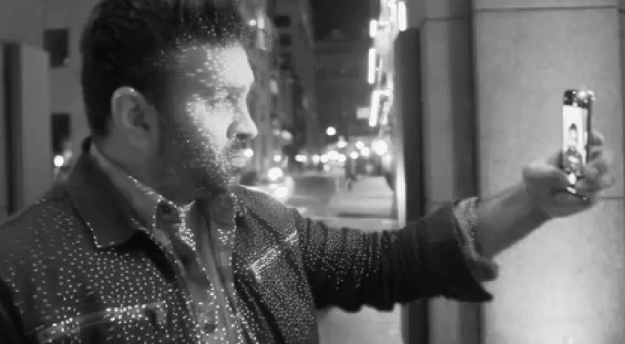 |
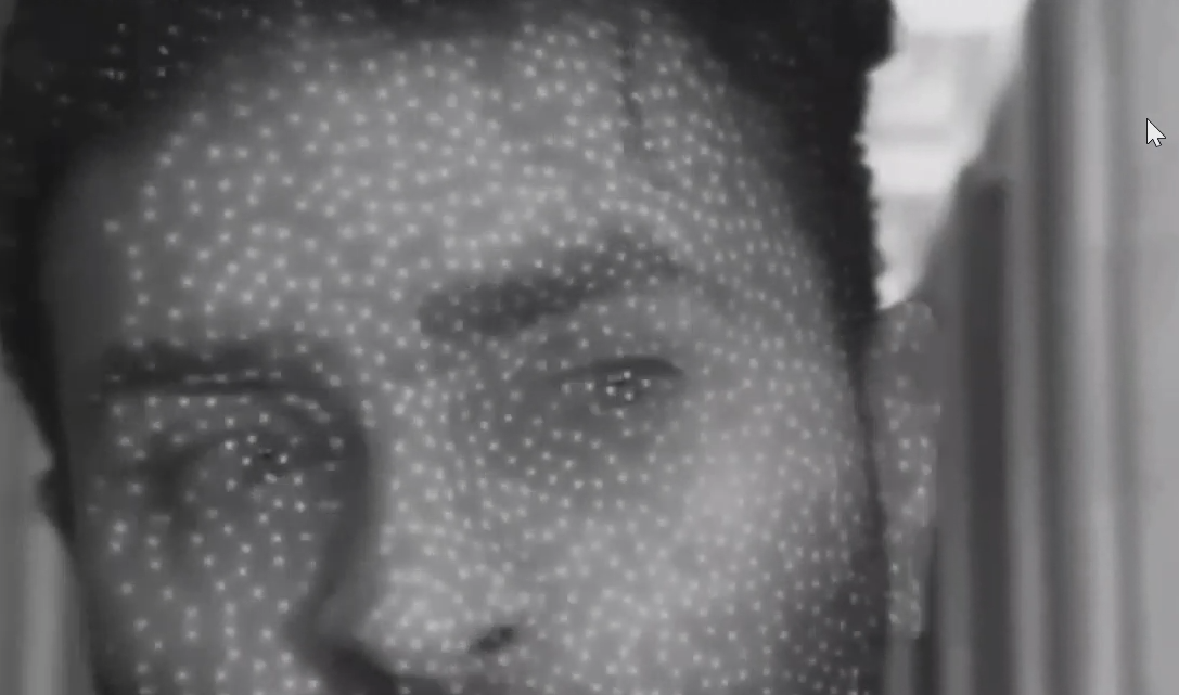 |
- how it works is that it shines infrared light on your face and you that to estimate depth
- our phones have many 3D sensors/streo cameras already!
LiDAR:
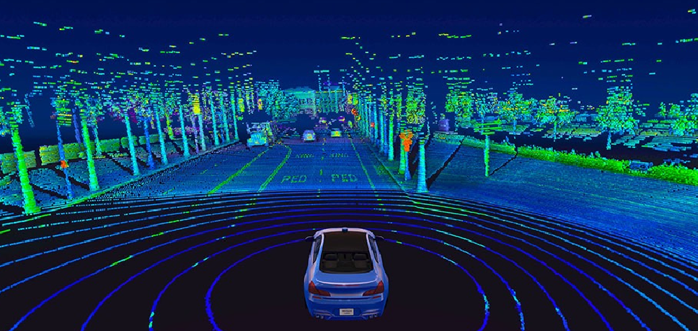
not using machine learning to compute depth, but uses laser to calculate depth.
-
essentially works by calculating how long the wave returns.
- basically the best sensor we have for outdoor depth estimation.
- it can see depth VERY far
- but many car manufactors uses camera instead of LiDAR. because
- it is too expensive!
- also there are cases when LiDAR doesn’t work. Since it is based on reflection time for wave, if you have rain and fog then it could reflect of from rain drops.
- last but not least, you still need cameras as it does not tell you what is there, but only depth
Representation of 3D Information
How do we represent this in machine?
- Images: Pixels
- Videos: Stop
- Motion Sound: Wave form
- 3D: how do we do it?
Essentially some ways to represent 3D information are:
- Voxel (volume Element): representing 3D scenes with many small 3D cubes
- Point Cloud: representing only object surfaces with a discrete number of points
- Mesh: the above but with surfaces connecting them, hence no holes
- Implicit Surface: by using a function $F(x,y,z)$ that given a coordinate gives you $0$ if you are in/on the object!
Voxel Representation
Recall how pixel representtaoin works
| 2D Images | 3D Info |
|---|---|
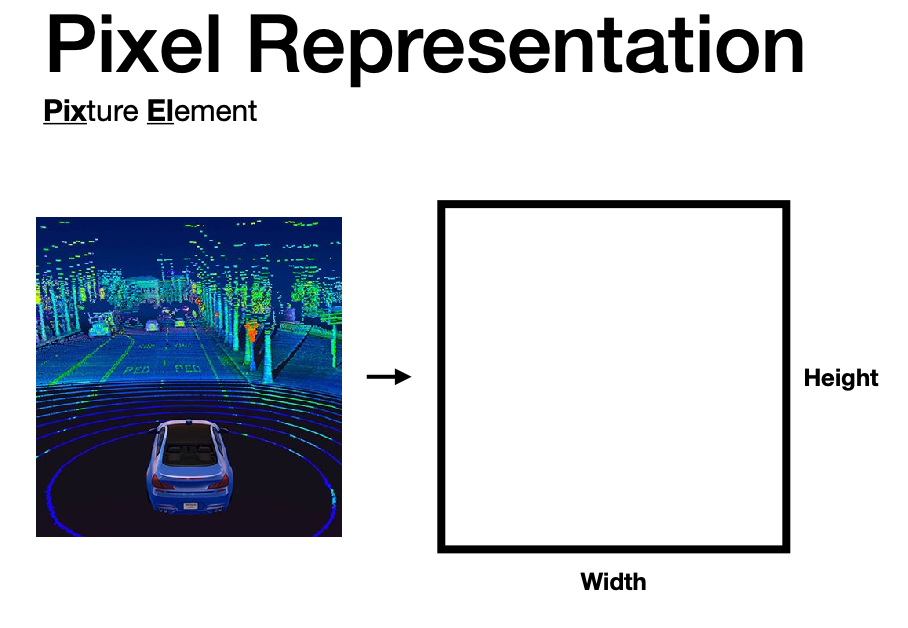 |
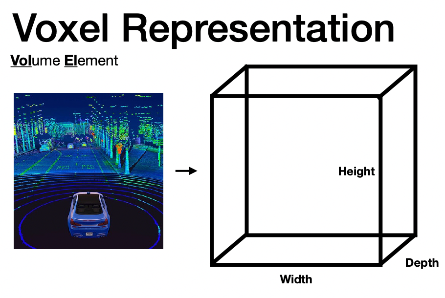 |
where if we have an object somewhere, we have a corresponding volume there.
-
basically like encapsulating the real world into the 3D box, so that if an object will be combination of volume elements in the space (like putting together a Lego)
-
but this is not used because
- it is too memory intensive . If we increase our “world”, it scales with $O(N^3)$
- it is often very sparse!
- there is also a trade of of resolution (i.e. the smallest volume component of an object) and details
- e.g. if your smallest Lego piece is very small, then you can have complex shapes. But if that is large, then you can only have simple shapes.
Point Cloud Representation
Consider to only represent objects (but not empty space), by using a collection of points on its surface
- resolves the sparsity problem as we only have objects represented
- and it also scales if we have a large scene!
| Representation | Example |
|---|---|
 |
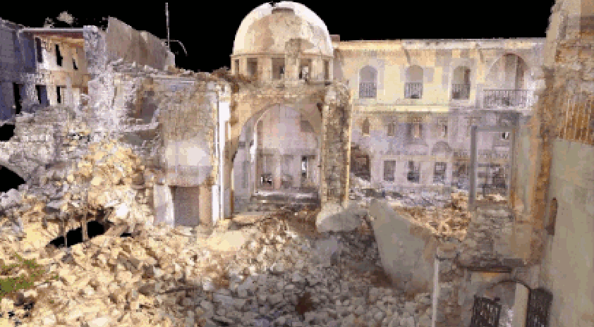 |
but there are problems:
- there are holes, which means you will need to interpolate in between if you need to model some interaction (e.g. robot picking up)
- the above worked because we have so many points, hence an illusion. If we zoom in, you see holes!
Mesh Representation
Instead of a collection of points, having them connected to form a mesh would resolve the “hole” problems
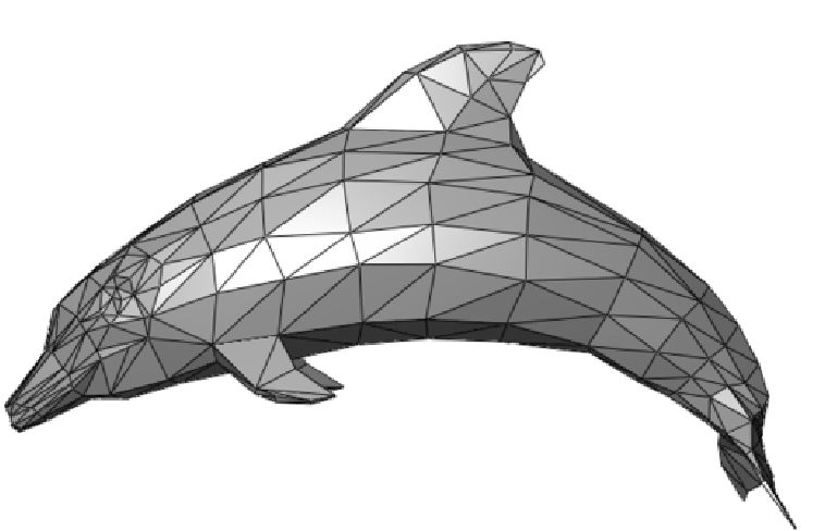
however, the problem is to integrade with neural nets
- it is easy to turn a lidar scan into a point cloud, but not a mesh
- why can we not just combine nearby points from a point cloud to a surface to get mesh?
- difficult to deal with noisy points. We need to determine whether if it is a noise and then decide to include it or not
- then we also need a merge algorithm, to merge the small surfaces into a larger smoother mesh
Implicit Surface Representation
Instead of modelling what we see, we can model a 3D shape by a function:
\[F(x,y,z) = 0 \iff \text{on surface}\]if it is not zero, it can represent the distance away form the object
- a very compact representation. You only need to store the parametre to the function.
- there is no resolution trade-off as everything is now continous! We can query any point we want (hence infinite resolution)
- but to get this function, e.g. we can train a NN to represent $F$. but it could be expensive to train
Essentially you can imagine this $F$ models the real world! (like the model-based method in RL algorithms)
Learnig with 3D Represnetation
Now, given a representation in either of the four, how do we perform tasks such as:
- classification of 3D objects
- segmentation of 3D objects by parts
- segmentation of a 3D scene
For example, if the input is point cloud representation:
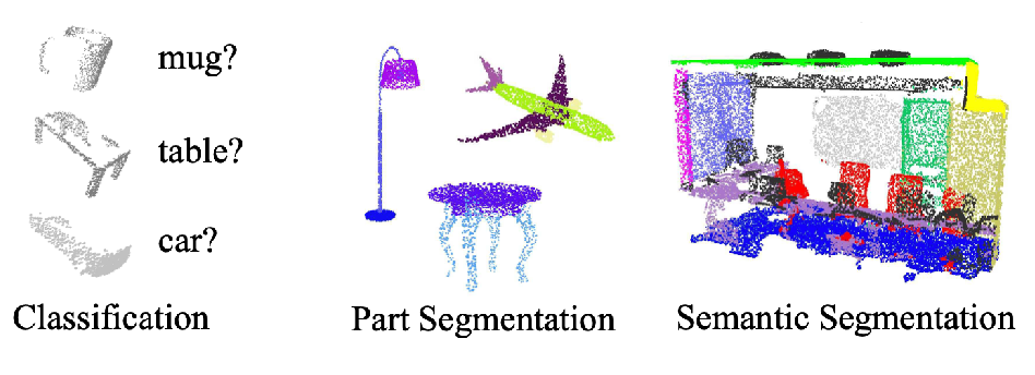
Learning with Point Clouds
Given some point clouds input, our task is to solve the following problems using ML:
Note that, as mentioned before, this representation have holes in the object, which we need to find some way to interpolate and know it is not empty space.
Since point cloud is essentially a list of coordinates:
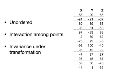
where consider we want to do object classification given this data:
- no-order in the data.
- for images we know which pixel is next to which pixel
- the above essentially enables convolution, we know neighbors of each pixel
- however, we do not have this information here!
- to recognize this as an object, we need to somehow learn interaction between the points
- we want our algorithm to be invariant under transformation
- if I shift everything over by 10, I would have not changed anything (because the center can be arbitrary).
- How do we make a NN learn those invariant transformation (e.g. still work produce the right classification)?
Some ideas you may have:
- first sort the data (deterministically), and then feed the results into a CNN. This is invariant to order!
- problem: will be disturbed by noise a lot
- problem: not invariant to rotation
- treat the order as data augmentation, then train a RNN
- problem: there are too many possible configurations to go through
- problem: still isn’t solving the invariance to order problem as we will only sample a limited orderings
- render this to a picture and then use CNN
- problem: lost all the 3D information such as viewpoints, occlusion.
PointNet Architecture
Idea: for each pooint $x_i$, we can extract some feature $h(x_i)$ by the same neural net, ant then have another function $g$ that is invariant to input so that we have:
\[f(x_1,...,x_n) = g(h(x_1),...,h(x_n))\]which is invariant to order by construction!
So essentially:
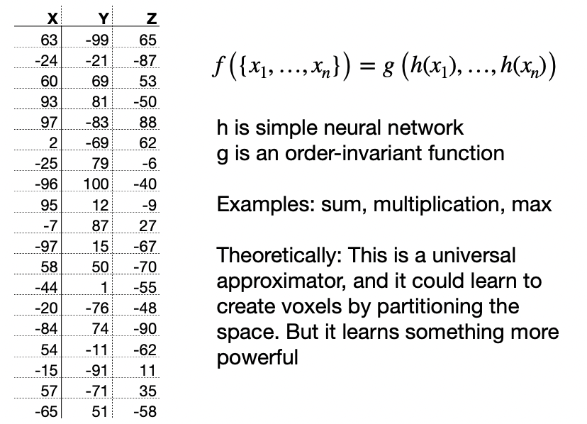
- each point goes through some NN $h$ to give a feature
- then the features goes into $g$, but this has to be order-invariant (e.g. sum/max)
- this this can be passed into some further NN as we are already order-invariant
- then our final resultant function is order invariant as well!
- however it is not invariant to transformation by construction
Then architecture looks like
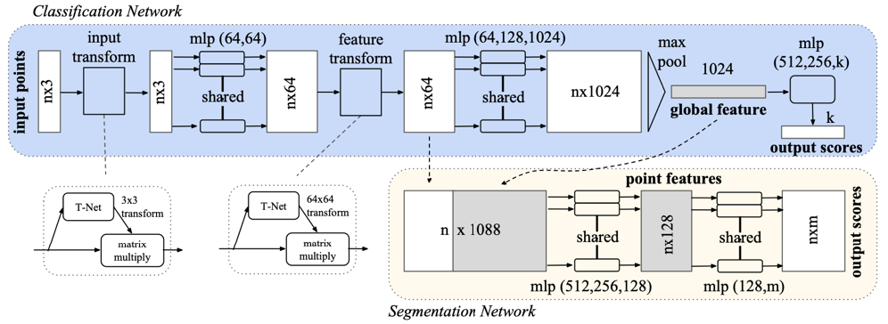
where:
- the global feature vector is essentially the output of the function $g$. Everything before that does some embedding of the input points are the function $h$, being marked as “shared”
- for segmentatoin, we needed to classify each point. Therefore it concatenates all the point features with the output hence giving a $n \times 1088$ matrix for classification.
- note that one limitation is that we need to feed in ALL points for input.
Some results of this architecture on classification and segmentation:
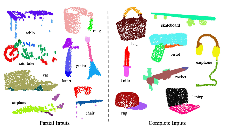
where we see that it works fine even if we have only partial point clouds
Critical Points
We see that in the network, a global feature is selected for classification:
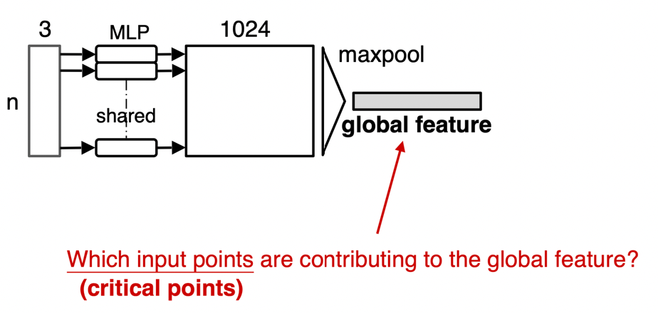
this means that
- there are some points that are useless (i.e. whether if we had them doens’t matter) for the current task (e.g. classification)
- therefore, if only a few points are useful for classification, we can visualize this by
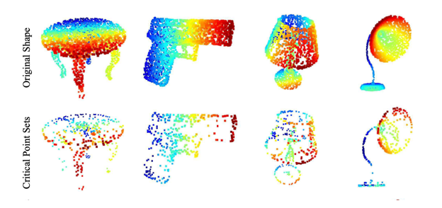
where we see that the bottom row are the kept points that the network used to do classification.
Learning with Implicit Surface
Recall that we want to learn a $F(x,y,z)$ that essentially models the scene we are given.
Idea: since this is a model, we can try to use this to do reconstruction of the original 3D scene and see if it matches
- note that since it only requires $x,y,z$, this means we already specified a camera view/hence coordinate space
- if we want to render scenes from a new coordinate space, this will not work
So essentially our overall architecture for training a NN to do $F(x,y,z)$ looks like
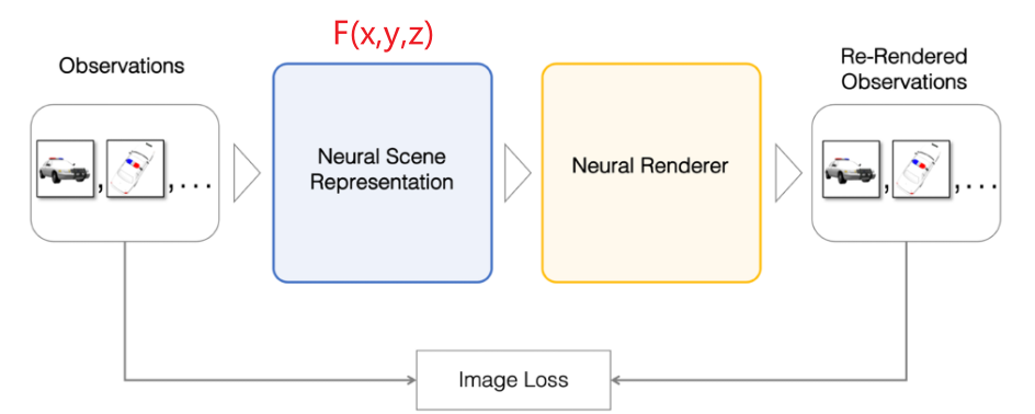
(note that the representation is conditioned on a certain camara view)
Training Scene Representation
Here we go into the details of how such algorithm works.
Essentially we want the scene representation network $F(x,y,z)$ to produce some information of the object/what to render when we give a coordinate. So essentially given some space
| Scene to Learn | Scene Model |
|---|---|
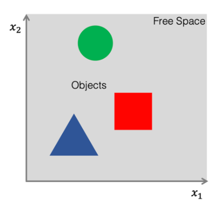 |
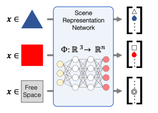 |
where
- grey means free space.
- Essentially we want to turn them into parameters such that, if we input coordinate of a blue triangle, output a feature vector that encodes the shape being triangle and color blue
How do we make sure we are modelling the scenes corectly?
Idea: have a decoder that queries this network $F$ and renders the scene accordingly. Then if $F$ does its job correctly, we will get a good reconstruction of the original 3D scene.
So basically the render (given a view point) iteratively computes the new scene by querying the network $F$
-
Basically it is a procedure of intersection testing. First it pick some point $x_0$ to render
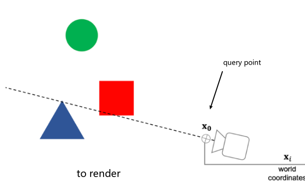
-
then it will query the network $F$ to know what is there to render
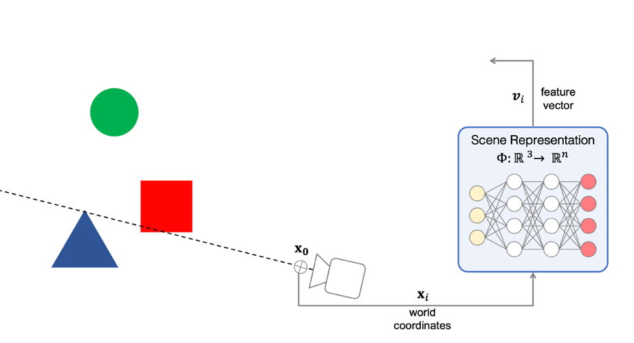
-
After rendered something based on $v_i$, consider what is the next point to query
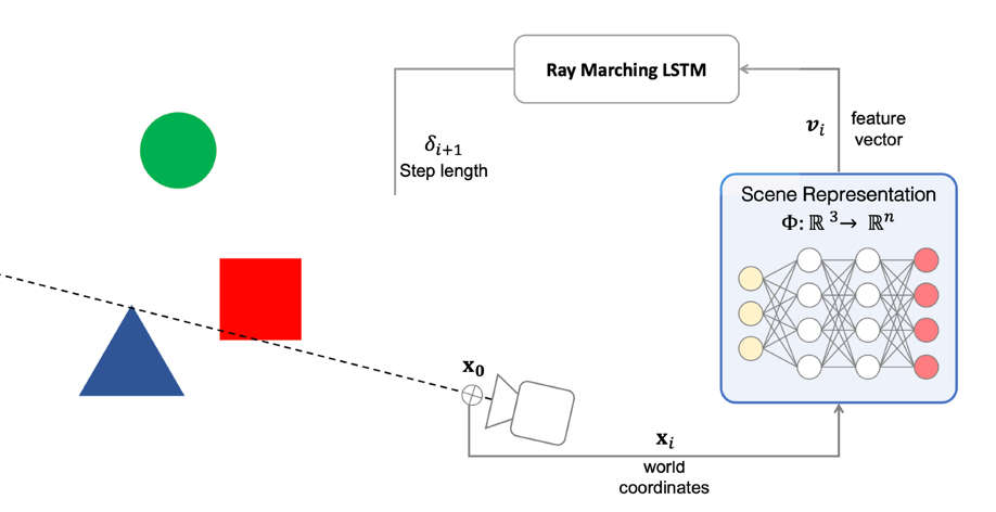
which is determined by outputing the step length $\delta$
- we used LSTM here because it needs to know the history of past queries for optimizing on what is the next step to pick
- this is useful as we have only a limited sampling time/iteration steps to render a scene
So then the next step looks like
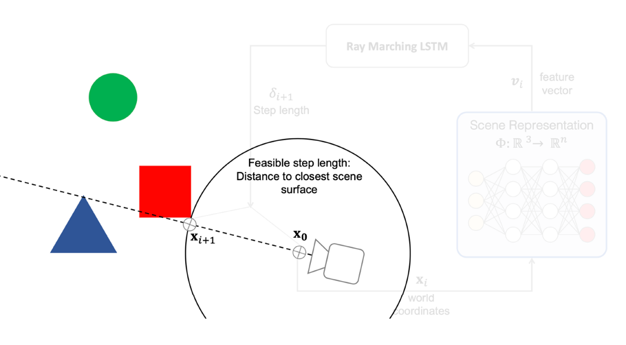
-
Finally, repeatedly do this until finish. The loss will be reconstruction loss.
Some results:
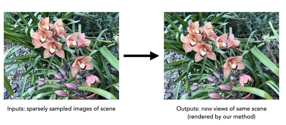
where in practice we might not have a 3D scene to start with. But we can start with a number of images taken on the same thing but different view points
- input will be a few samples of the same object, then output synthesized views from any camera views
Neural Radiance Fields - NERF
the model worked by specifying some coordinate system/camera view to begin with. What if we want to also produce a model $F$ such that it can render different camera views?
So essentially we will have our model being
\[F(x,y,z,\theta,\phi)\]for $\theta,\phi$ specified our view point. Hence our network becomes:
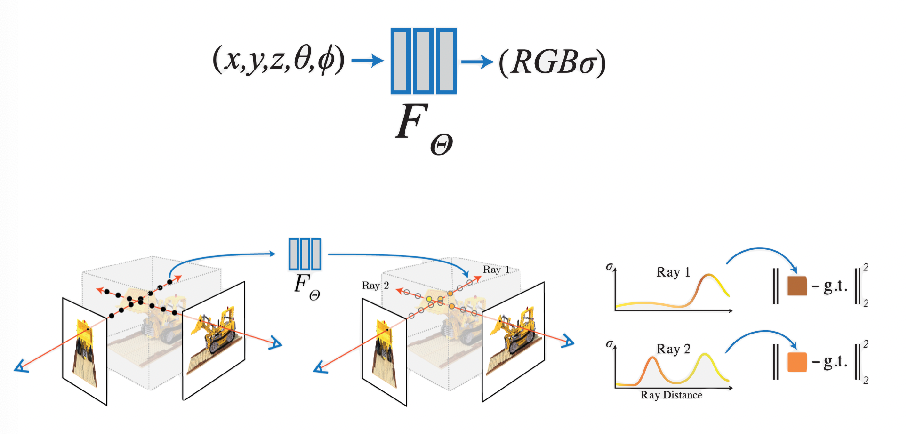
then results look like
| Input Scene | Output View 1 | Output View 2 | Output View … |
|---|---|---|---|
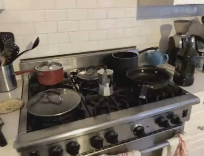 |
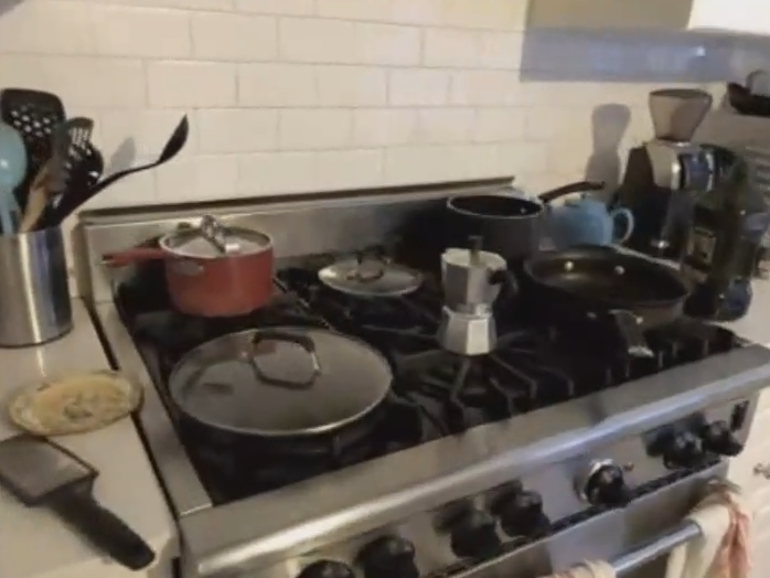 |
 |
so that basically the “world model” then also spits out lighting information/reflection now!
Final Exam
Final exam next class:
- grade scope exam releaieas at 10:15
- need to joing zoom and have camera on without virtual backgrounds
- length is 90 minutes
- open notes, open slides, etc.
Some topics:
- fourier transform
- back propagation
- object recognition
- motion and hyperbolic geometry