Deep Learning Part 2

Automated Machine Learning

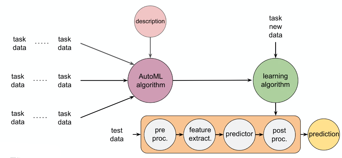
The idea is to, given some task and its dataset, find a ML algorithm (including the five pieces shown below) that solves a problem

where the training data/task/solution could come from Kaggle, as a label composed of the following 5 pieces:

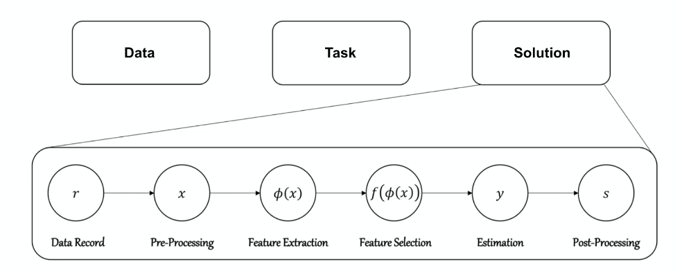
pre-processing: which imputation method if needed?
feature extraction: which encoding to use? backbone?
feature selection: should we do dimensionality reduction?
model/predictor: which classifier?
post processing

Such an idea of automatically finding best tools could be applied to a range of similar tasks such as:

automated activation function finding:

where essentially we given in building blocks to compose some activation function, and ask it to find a best one
automated optimizer finding, where again we feed in building blocks for an optimizer

and under some tasks, the best solution could be:
\[\text{PowerSign} = \alpha^{f(t)*\text{sign}(g)*\text{sign}(m)}*g\]
for $g$ being gradient and $m$ being momentum.
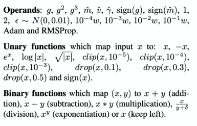
automated data augmentation finding. Again, consider a space of possible actions:
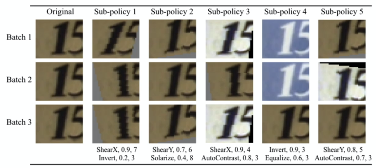
automated algorithm selection
automated hyperparameters finding: Grid Search v.s. Random Search
automated architecture finding
and etc.

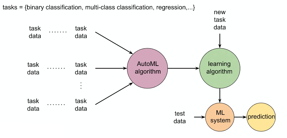
AutoML

The idea is to have:

input some task + data of a problem
output a ML system that you can use to do predictions

Some nowadays implemented ones look like:

autosklearn

import autosklearn.classification # classification task
cls = autosklearn.classification.AutoSklearnClassifier()
cls.fit(X_train, Y_train)
predictions = cls.predict(X_test)

flaml
h20
etc.

Note that this of course does not really find the best tuning of the model, it only finds some pipeline/architecture. To find the best hyperparameters, checkout the section on Automated Hyperparameter Finding

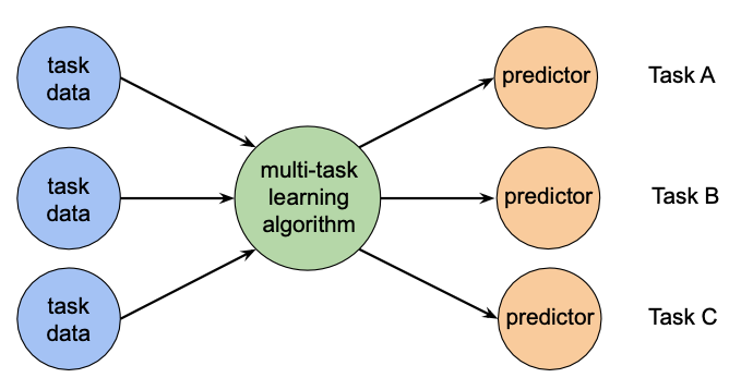
Meta Data

How do we represent the task/dataset/solution as a feature in the AutoML system?

Instead of putting the entire task/dataset as it, consider computing some meta data about the task/dataset/solution.

Hence we consider:

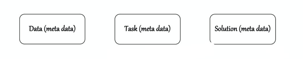
for instance, metadata features for dataset include:

number of data points
number of features
number of missing values
class entropy
etc.

Hyperparameters Finding

Certain hyperparameters we commonly care about are:

learning rate $\alpha$
momentum $\beta$
minibatch size
learning rate decay
etc.

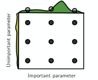
The easiest approach is to consider grid search. However, this is often inefficient as it assumes each parameter being equally important.

Grid Search	Random Search

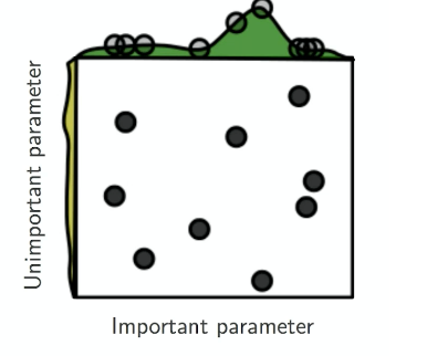consider random search

not all hyperparameters are equally important. For example, lr might be more important than decay coefficient $\gamma$.
if you look at the range of values covered by important parameter, grid search only searched $3$ possible values, whereas random search searched $6\sim 7$ different values

Several other ways include:

adaptive search in certain regions where we found good candidates:

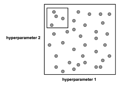
i.e. make the search more dense in that area
converting the problem to a RL task. Consider this as a multi-arm bandit: we pull an arm (sample in the hyperparameter space), the reward is the performance/training time, etc
Bayesian optimization. see section Bayesian Optimization.

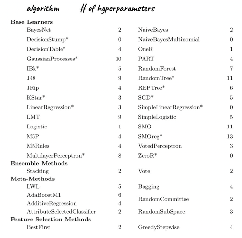
Algorithm and Hyperparameter Selection

Instead of finding the algorithm and the hyperparameters, consider finding them jointly.

Given a dataset $D$, find the algorithm $A$ (e.g. linear regression, decision tree, etc) and a hyperparameter such that we minimize the loss of $A$ on $D_{test}$ when trained on $D_{train}$:

\[A^*_{\theta^*} = \arg\min_{A,\theta} \sum \mathcal{L}(A_\theta, D_{train}, D_{valid})\]

The algorithms and hyperparameters you can search through could be:

Ensemble of Models

Idea: When you have multiple potential models for a single task, instead of choosing one single model, we can keep all models.

The simplest ensembling is the following: given a test sample point $x$:

for each model $m$: perform prediction for probability of $x$ in the $j$-th class, i.e. $p^{(j)}$
for each class $j$: do averages of probability for each model
take $\arg\max_j$ to split out the prediction

\[y = \arg\max_j \frac{1}{m} \left( \sum_{i=1}^m p_i^{(j)} \right)\]

This would be the simplest form of assembling. Other ways would be stacking

Model Stacking

One problem with performing the simple ensemble above is that, for a new given test data $x$, you will need a central place to store all the models. This might not be efficient and desirable.

Goal: is there a way to collaborate without sharing a central repo for code/models?

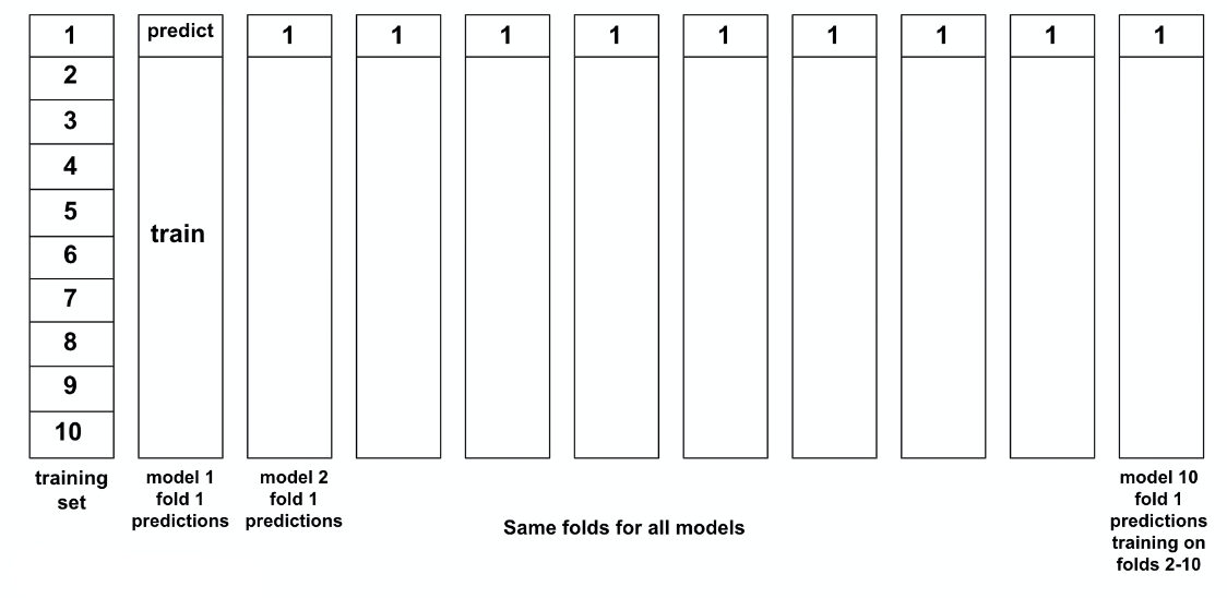
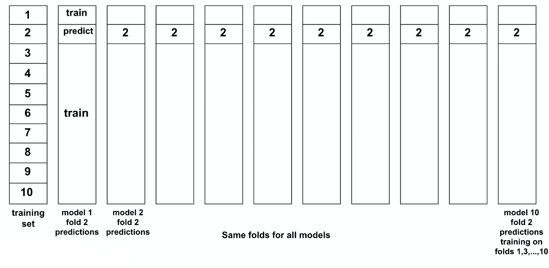
Idea: consider building a super model that trains on outputs of each model.

This means that, for each model $m$:

define the same CV folds for all models
ask each model to keep the predictions for each fold $i$.

CV Fold 1	CV Fold 2

Then the idea is to take the predictions from each model as a meta-feature that you can feed in to a super-model:

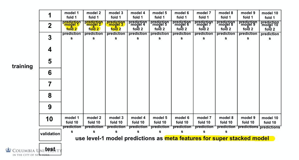
The key idea is so that:

we only need each team for model $m$ to work on their own
building a super model then is just build a model, we don’t need to look into codes of other teams

Neural Architecture Search

Developing novel neural architectures manually is time consuming, error prone. Now you can use automatic methods for searching for neural network architectures: AutoKeras (CNN, RNN), AutoGAN, AutoGNN.

For deep learning models, we might consider combining many different algorithms in a pipeline such as CNN as backbone and then Transformers.

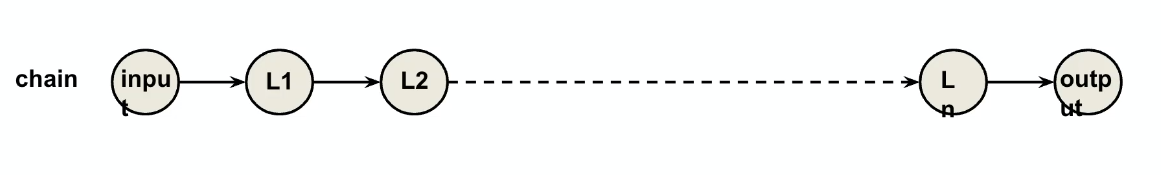
Most packages cover two possible architecture shape:

Chain	DAG

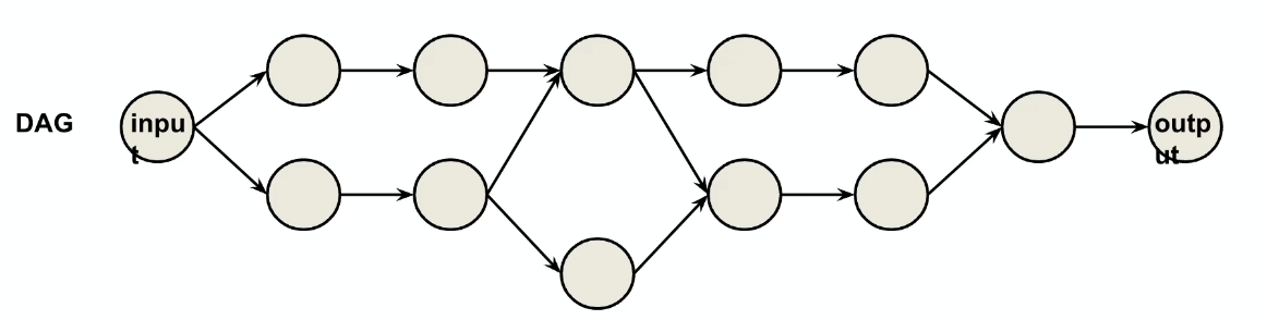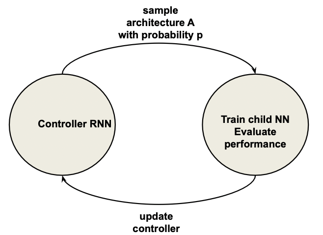
However, another approach would be a RL like task:

ask NN controller to generate an architecture (take action)
evaluate performance (get reward)
get feed back to NN controller (update)

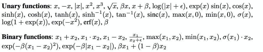
DARPA

DARPA Data Driven Discovery of Models (D3M): solve any well defined ML task on any dataset specified by a user.

Broad set of computational primitives as machine learning building blocks.
- e.g. implementing PCA, Linear layers, etc.
Automatic systems for machine learning, synthesize pipeline and hyperparameters to solve a previously unknown data and problem.
- given a test dataset and task in a Docker image, ask your code to generate a model and predict
Human in the loop user interface that enables users to interact with and improve the automatically generated results.
- maybe user only wants a subset of models to choose from, etc.

The outcome from such a project are two methods where you either:

Gradient-based: have differentiable primitives, build a DAG, and optimize end-to-end using backprop:
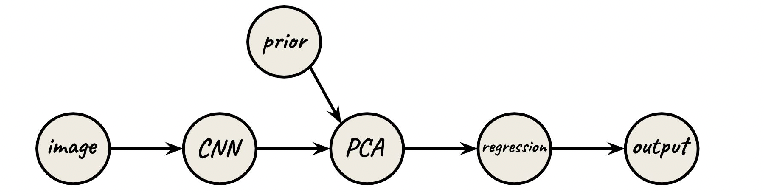
Reinforcement-based: since essentially it is a search in high dimensional space,

Idea Parallel in RL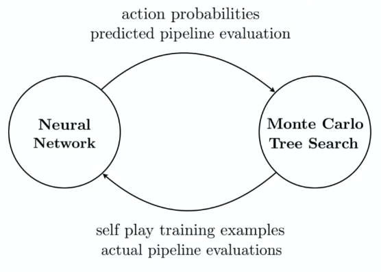

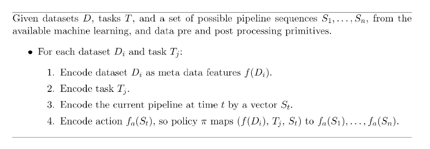
in this approach, the entire pipeline is a single state. Therefore we need some kind of encoding for the pipeline, which can be done by:

A brief comparison on performance

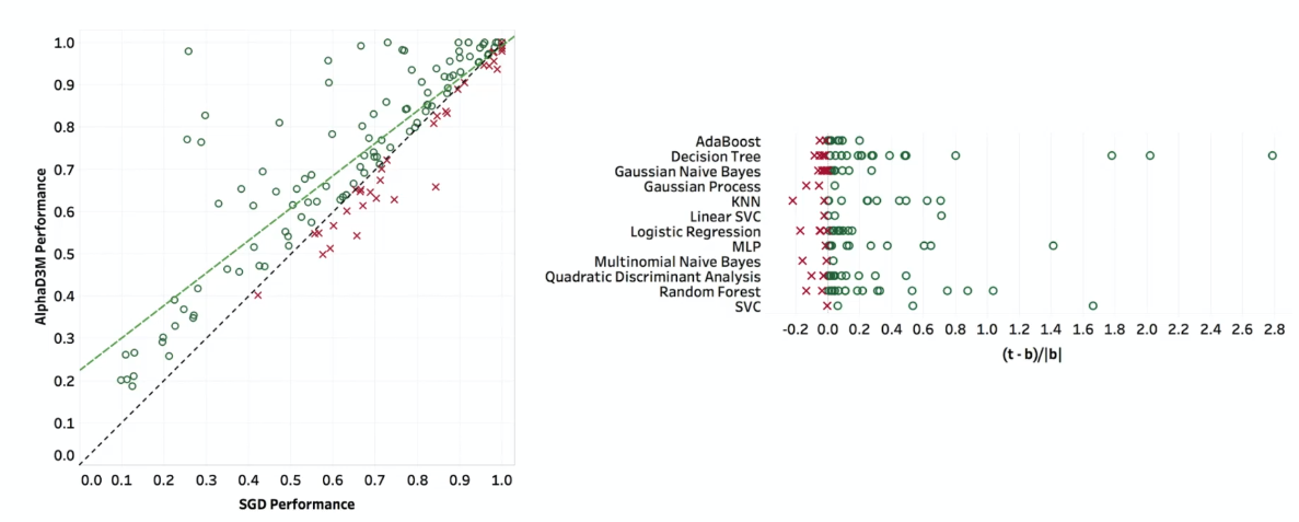
where the horizontal line is the gradient-based method, we see that RL-based in doing better.

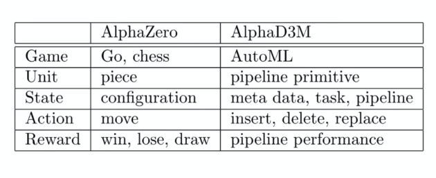
RL-based Pipeline Synthesis

Recall that

Deep RL	Pipeline Synthesis

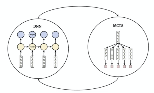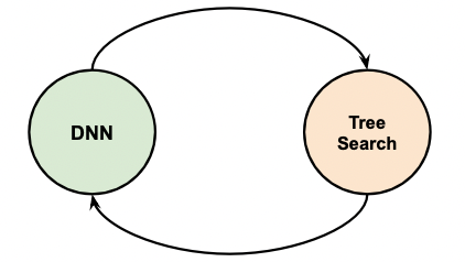
where essentially:

DNN now receives an entire pipeline, meta features and task as input, and estimates action probabilities as well as rewards, i.e. performance
MCTS then receives the data from DNN and search for next action
an action here would be modification/insertion/deletion of a certain primitive in the pipeline.

However, this tree search by default could also hit on certain meaningless pipelines such as estimator and then preprocessing. Hence you can enforce a grammar to only accept valid ones, i.e. giving some prior knowledge.

The performance becomes better

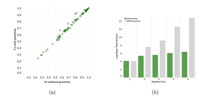
In the end, an ablation study is done on using the DNN or not. The result is similar but time performance is drastic

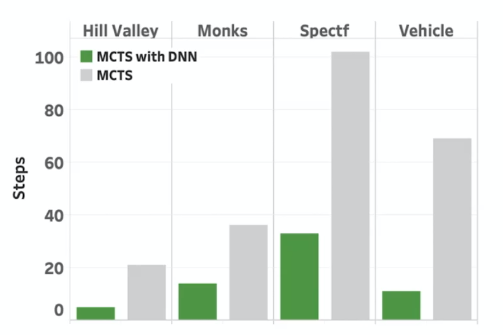
basically just MCTS would be very slow.

Matrix Completion and AutoML

It turns out the idea behind AutoML can be extended to/related to many applications in real life.

Another task would be a recommendation system, where given some past user’s ratings/history, fill in how likely users will like a certain film.

The problem can be setup as a matrix:

each user being $j=1,..,p$
each item, e.g. movie, being $i=1,…,n$
each cell represent rating $Y_{ij}$ a user $j$ gave to item $i$

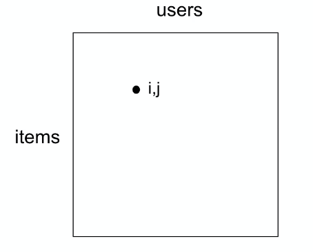
where this would be a sparse matrix in general as many users won’t see all contents.

the task is then to complete the matrix, so that we can perhaps recommend to users

In terms of AutoML, we are basically doing:

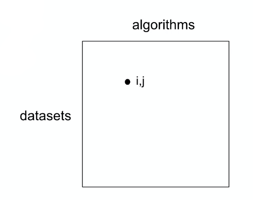
where if fully filled, we can find the best algorithms given a dataset.

Naive Solution of Filling Matrix:

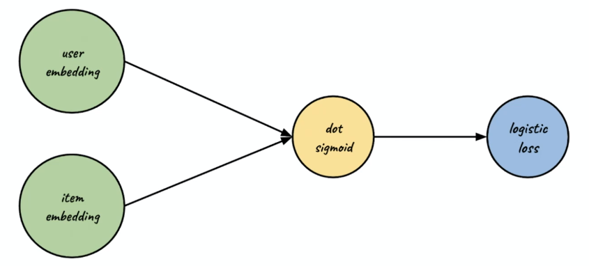
Let each item have a known feature vector $\vec{x}^{(i)}$. We want to learn some parameters $\theta^{(j)}$ of each user and assume that $\theta^{(j)^T}x^{i}$ would model their preference score. Then:

\[\min_{\theta^{(j)}} \frac{1}{2} \sum_{i:M_{ij}=1} \left(\theta^{(j)^T}x^{i} - Y_{ij}\right)^2 + \text{Regularize}(\theta^{(j)})\]

note that since we only know part of the matrix:

$i:M_{ij}=1$ means we are only fitting on the known parts
then we can predict once we learnt $\theta^{(j)}$ for each user $j$

This model is actually the simple content-based recommendation system

Problem: In tasks AutoML needs to solve, we are usually given a unknown/new dataset and task. I.e. we are having a new item with unknown $\vec{x}^{i}$.

Then, the idea is to do a EM-like approach:

assume you know $x^{(i)}$, fit $\theta^{(j)}$
then once you get $\theta^{(j)}$ fit $x^{(i)}$ back

So the entire task can be seen as

\[\min_{\theta^{(j)},x^{(i)}} \frac{1}{2} \sum_{i:M_{ij}=1} \left(\theta^{(j)^T}x^{i} - Y_{ij}\right)^2 + \text{Regularize}(x^{(i)}) + \text{Regularize}(\theta^{(j)})\]

which then we can fill in all items in the matrix. Note that:

this model only using dot products can be rephrased into a lower rank decomposition and imputation

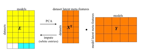
The upshot is that for AutoML, we can keep past experience with different dsets and architecture as elements in the matrix, and treat the matrix as a warm start for MCTS search. (i.e. use that as initialization)

Using Meta Embeddings

When approaching an ML or DS problem humans read the documentation

Description of data and task
Description of machine learning functions available for solution
How can we allow an AutoML method to “read the descriptions or manual”? (in addition of the actual datasets)

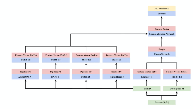
Use large scale transformer models to represent descriptions of the dataset, task, etc, in addition to the dataset itself.

It turns out that just using the metadata could do equally well even if you haven’t seen the actual dataset

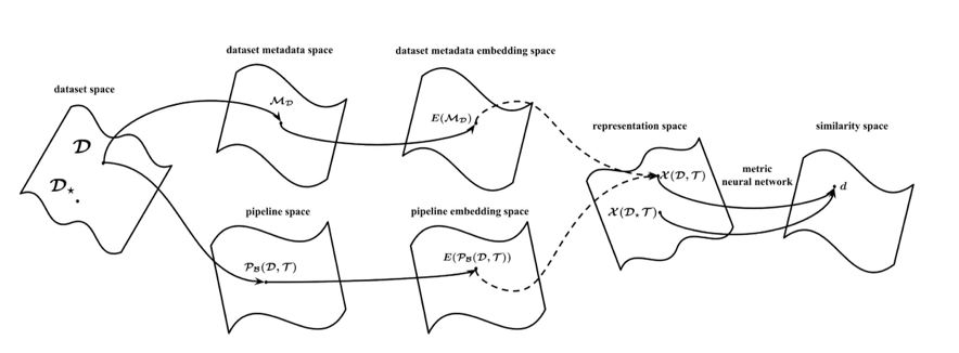
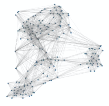
One potential representation would be computing a graph embedding: embedding of dataset that are similar should be close.

Dataset Embedding	AutoML Architecture with Meta data

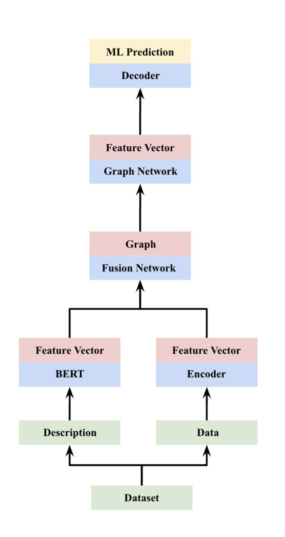where:

nodes in a graph would represent a dataset
edge would be based on embedding of dataset descriptions and meta-features
this is bascially the approach now: using GNN combined into AutoML systems

Then you use assembling to those AutoML systems as well

Bayesian Optimization

Here we cover another popular technique other than random search and grid search for hyperparameter selection.

Goal: Given some model and a loss function, select model hyperparameters such that the loss would be small.

We would want:

\[z^* = \arg\min \mathcal{L}(M_z)\]

and we want to approximate best hyperparameter $z^*$ that minimizes the loss within only a few steps $z_1,…,z_n$.

The idea is:

have some prior on the objective function, say $f$, which could be the loss/some performance metric
each time we evaluate $f$ at a new point $z_i\equiv x_i$, we update our model for $f(x)$
use posterior to derive/update acquisition function $\alpha(x)$
\[\alpha(x) = \mu(x) - k \sigma(x)\]
where $\mu(x),\sigma(x)$ are mean and std. of posterior at point $x$. Here $k$ controls the trade of between exploration and exploitation:
- if small $k$, then the $\arg\min$ in the next step favors small $\mu(x)$, o.e. exploitation
- if large $k$, then exploration
use the acquisition function to determine the next point
\[x_{i+1} = \arg\min \alpha(x)\]
and continue from step 2

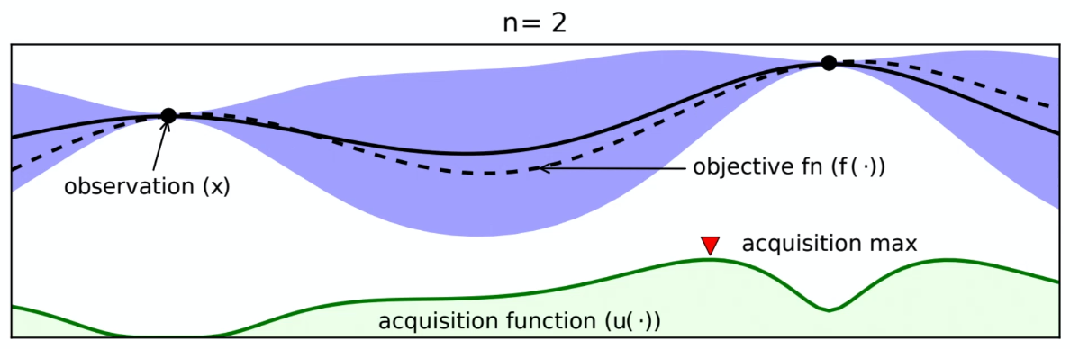
Graphically, suppose we have already sampled three points $x_1,x_2,x_3$, e.g. learning rate. We are interested in which point to sample next:

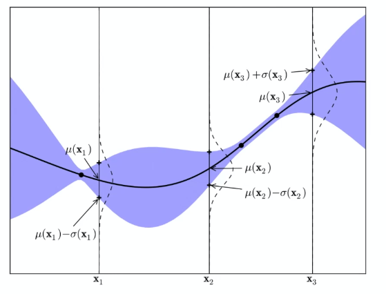
where

the blue part would be the confidence intervals
the black line would be the true function which we don’t know

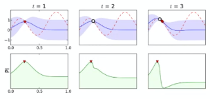
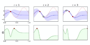
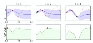
Now, depending how we choose $k$, the acquisition function could look differently:

For instance:

Exploitation	In between	Upper Confidence Bound

where the

exploitation would result in $x_{i+1}$ in lower confidence bound

The algorithm hence looks like

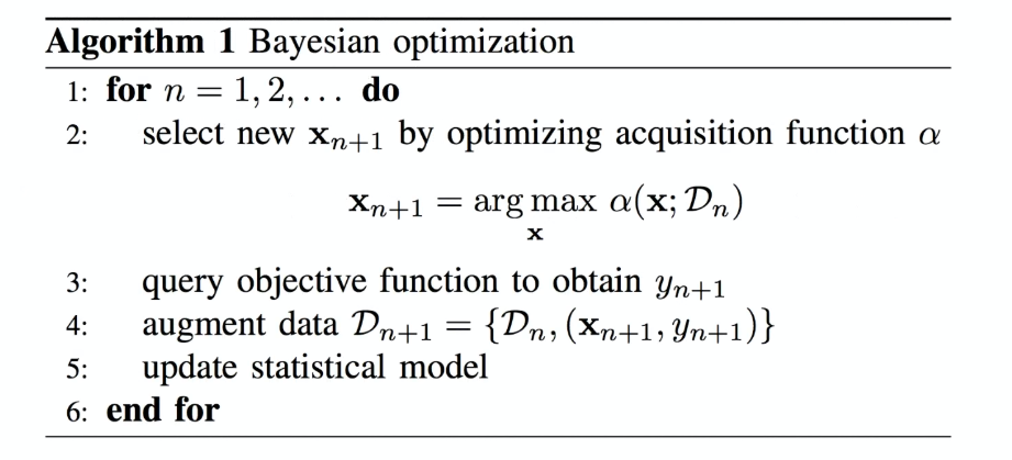
And in practice, sklearn already implemented such a search. It has a function which uses a flag to either do Grid Search, Random Search, or Bayesian Optimizations.

Multi-Task Learning

In the real word, solving a problem = solving many tasks at the same time.

For instance, consider self-driving cars

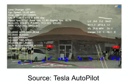
where we need to do:

object detection for pedestrians, other cars, etc
RL learning driving
dehazing if needed
etc.

Some questions we want to answer here include:

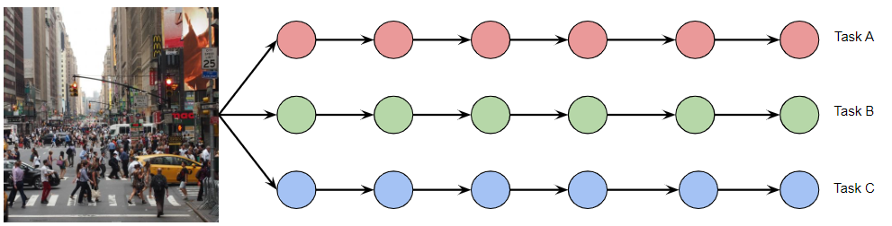
do we want to build predictors doing independent work for each task?
independent predictors but using the same backbone?
or maybe one model for all tasks? i.e. one neural network for learning multiple tasks: all-in-one

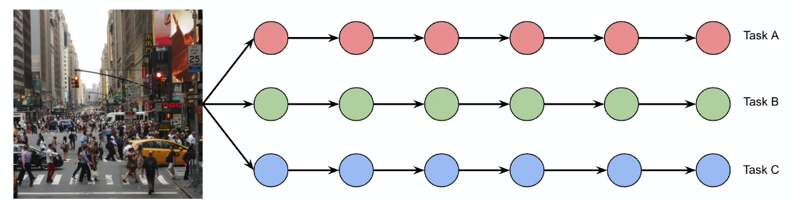
Independent Network

The simplest approach for solving $N$ different task would be to have the following architecture

Some advantages

simple to build
do not need to

some disadvantages

no sharing hence no positive transfers
not resource efficient

Positive Transfer refers to the facilitation, in learning or performance, of a new/second task based on what has been learned during a previous one.

Negative transfer refers to any decline in learning or performance of a second task due to learning a previous one.

Multi-Task Learning Questions

In reality, we have multiple heterogeneous tasks with different importance, difficulty, number of samples, noise level

Some questions you might think about to develop an architecture:

How do tasks influence one another? Does each task help the other tasks? or is there negative transfer?
- e.g. if we train backbone + detection head 1 on pedestrian detection, will it hurt the performance for same backbone + detection head 2 on car detection?
- Are the tasks similar? Heterogeneous?
How to share weights between different tasks?
- e.g. shared backbone? Layer Routing?
How does network size influence MTL?
How does dataset size and distribution of number of samples per task influence MTL?

Zero/One/Few Shot Learning

This is relevant in transfer learning. I.e. suppose you have fitted your model on some data from domain $D_A$. You want to see how well it can perform on a different domain $D_B$:

Few-shot learning aims for ML models to predict the correct class of instances when a small number of examples are available in the $D_B$.

$N$-shot learning aims to predict the correct class when $N$ examples for each class in the $D_B$.

Zero-shot learning aims to predict the correct class without being exposed to any instances belonging to that class in $D_B$.

In general you have $k$-shot $n$-ways, for $n$-ways being the number of classes.

Why is this relevant? One way to see it is that if our model can perform well on few/one-shot, then:

all we need is a single model with a few-shot examples to solve multiple tasks.

Advantage: models trained on multiple tasks at once are more robust to adversarial attacks on individual tasks
Disadvantage: hard to get it to work

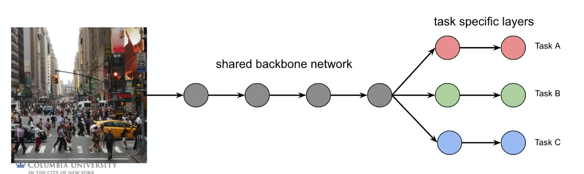
Shared Backbone

Consider the setup of:

input $x$
need to solve $T$ tasks, $t=1,…,T$
output of each task is $y_t$

Suppose we are given $N$ training data, being ${x^{(i)}, y_1^{(i)},…, y_T^{(i)}}_{i=1}^T$. We consider the architecture of

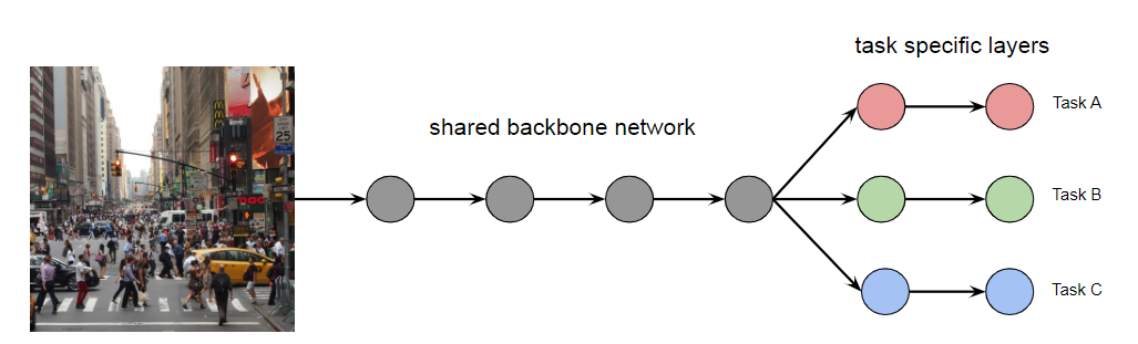
where

again the backbone would take the role of feature extractor
we can also see this as the backbone being “encoder”, and the three tasks being three different “decoders”
Advantages: efficient runtime
Disadvantages: could be over-sharing, negative transfer

Then specifically, we have:

shared backbone network $f$ with parameter $\theta_s$
task-specific decoder network would be $g_t$ for each task $t$, with parameter $\theta_t$
task-specific loss would be defined as
\[\mathcal{L}_t(\theta_t, \theta_s)=\frac{1}{N}\sum_i \mathcal{L}_t(g_t(f(x;\theta_s);\theta_t),y_t)\]

Note that though for each task you can define your own loss, what happens when we update $\theta_s$? There will be $T$ different losses for a single $\theta_s$. How do we update that?

Linear Scalarization of MTL

Aim: we want to solve for the best combination of all parameters $\theta_s$ and $\theta_{t_1},…,\theta_{t_T}$.

The problem we are considering is the following and we want to solve for the best $\theta$ set:

\[\min_\theta \mathcal{L}(\theta)\equiv\min_{\theta_i} \mathcal{L}(\theta_s,\theta_{t_1},...,\theta_{t_T})\]

But the key problem here is that solutions may not be comparable to begin with:

consider $\theta,\theta’$ being two sets of solution such that
\[\mathcal{L}_{t_1}(\theta_s,\theta_{t_1})<\mathcal{L}_{t_1}(\theta_s',\theta_{t_1}')\]
so that this the $\theta$ set performs better in task 1, but
\[\mathcal{L}_{t_2}(\theta_s,\theta_{t_2})>\mathcal{L}_{t_2}(\theta_s',\theta_{t_2}')\]
in task 2, the set $\theta’$ performs better.

Therefore, how do we define an ordering for the parameters to begin with?

One simple idea is to consider a linear combination

\[\mathcal{L}(\theta)\equiv \mathcal{L}(\theta_s,\theta_1,...,\theta_T) \to \sum_t \alpha_t \mathcal{L}_t(\theta_t,\theta_s)\]

which gives a well-defined ordering. Then we can update/solve by:

\[\min_{\theta}\mathcal{L}(\theta) =\min_{\theta} \sum_t \alpha_t \mathcal{L}_t(\theta_t,\theta_s)\]

but how do we find an $\alpha$?

Multi-Objective Optimization

Another formulation/view point of the task is to consider

\[\min_{\theta_i} \mathcal{L}(\theta_s,\theta_{t_1},...,\theta_{t_T}) = \min_{\theta_i}(\mathcal{L}_{t_1}(\theta_s,\theta_{t_1}),...,\mathcal{L}_{t_T}(\theta_s,\theta_{t_T}))\]

This can be generalized into the question that we have a system of $T$ functions $f_t(x) = \mathcal{L}(\theta)$, then we can define a partial ordering for $y \in \mathbb{R}^T = (f_1(x),…,f_T(x))$ such that:

\[y \prec y' \iff f_i(x) < f_i(x')\,\,\forall i\]

in other words, $y$ wins/is smaller if it is smaller in all dimension. Then applied in our case, we essentially have “many optimal solutions” forming a Pareto frontier.

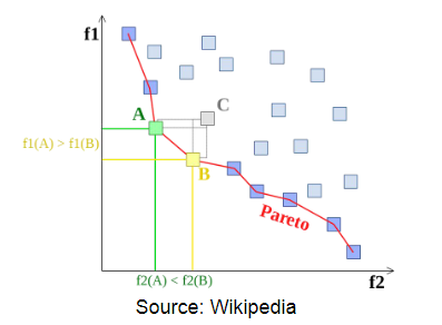
where notice that:

$A,B$ are pareto frontiers since no other point can perform better than them in all dimension, $f_1, f_2$ in this case.
$C$ is not because it could be out-performed by $A,B$ in both dimensions.

Theorem: All pareto optimal points are Pareto stationary.

Theorem: A point $x$is pareto stationary if there exists $\alpha \in \mathbb{R}^T$ such that
\[\sum_t \alpha_t \nabla f_t(x)=0,\quad \sum_t \alpha_t=1,\forall\alpha_t \ge 0\]

Therefore, this gives us a way to define how to find a meaningful $\alpha$, which comes down to:

\[\min_\alpha \left\| \sum_t \alpha_t \nabla f_t(x) \right\| \to \min_\alpha \left\| \sum_t \alpha_t \nabla \mathcal{L}_t(\theta_s, \theta_t) \right\|\]

under the constraint that $\sum_t \alpha_t=1,\forall\alpha_t \ge 0$.

Negative Transfer

Up to today, individual networks are performing better than shared networks.

The cause is mainly due to negative transfer happening:

One task may dominate training
Tasks may learn at different rates
Gradients may conflict

So in general it is important to determine the relationships between tasks, to tell if a shared architecture works

Architectures in Shared Networks

In general we have:

Hard parameter sharing, which we have seen
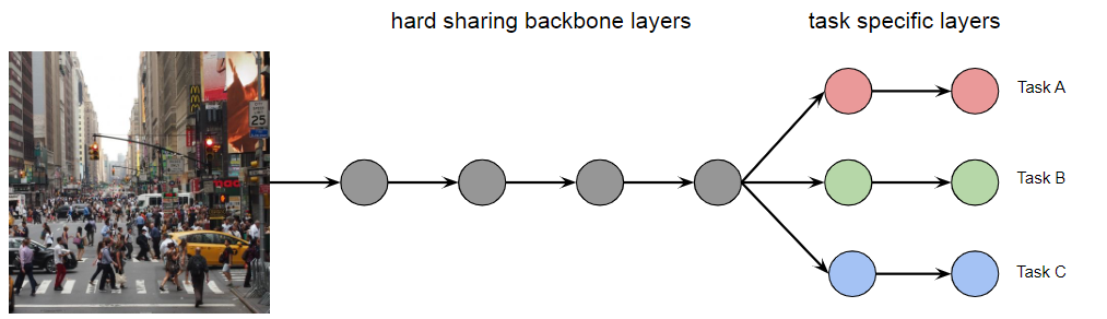
Soft parameter sharing

Instead we can imitate individual networks but allow sharing:

Hard Sharing Soft Sharing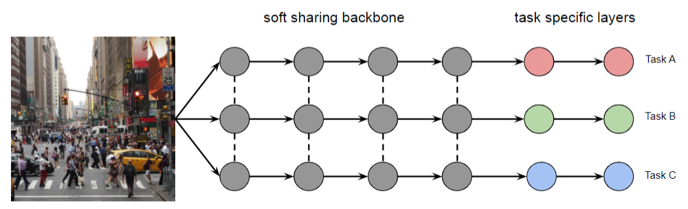

Does not scale well with number of tasks
Ad-hoc sharing

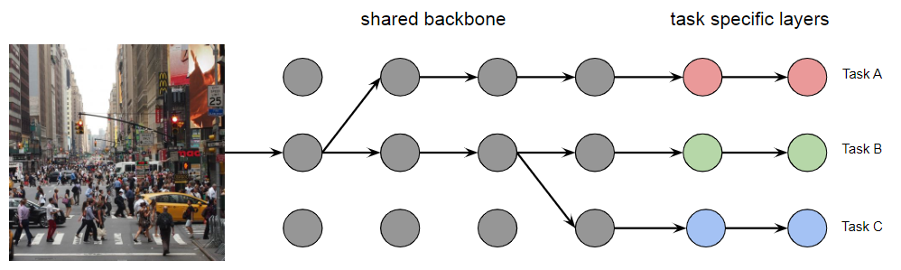
so we compute task relatedness, then iteratively group network

This tend to have better performance than soft or hard sharing
learning to route

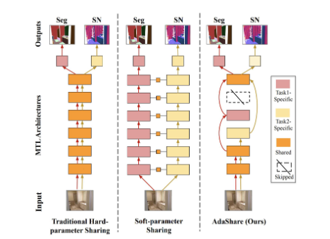
where we learn separate execution paths for different tasks

Combinatorial Optimization Problem

Which Tasks Should Be Learned Together in Multi-task Learning? If we want one model doing more than one thing?

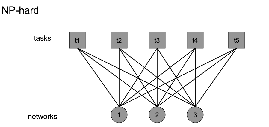
Consider this problem as a bipartite matching

Problem	Approximate Solution

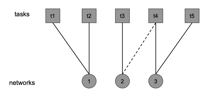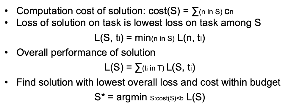
Then the question can be formulated as:

Tasks being $t_1,…,t_T$ having $T$ nodes
NN Network having $n$ nodes, each would have a cost to use $c_n$ (e.g. inference time)
we have a budget $b$, which we do not want to exceed (e.g. should not take longer than $b$ seconds)
want to have a solution $S$ being a set of network using the $n$ nodes that solves all $T$ tasks within the budget

Then this problem is:

where of course this is still a NP-hard problem, so in reality we would use approximations. Some results look like

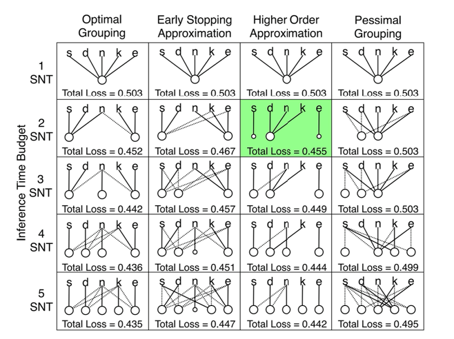
where $S,D,N,K,E$ would be the tasks, and the circular nodes are the networks.

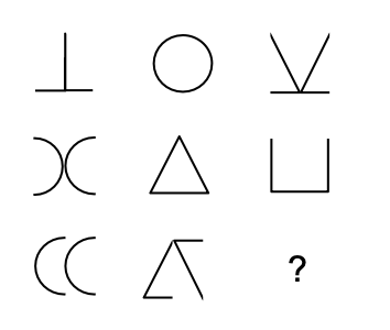
Example: Raven’s Progressive Matrices

The task of Raven’s Progressive Matrices is to fill in the missing patterns.

Question	Answers

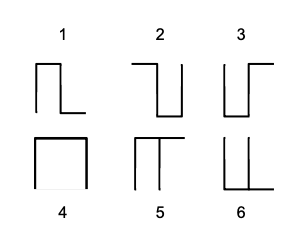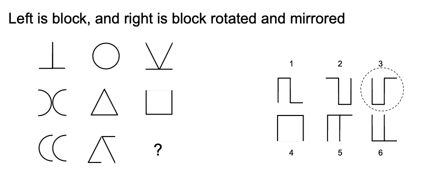
notice that this is a multi-task question. We need to

infer hidden attributes and pattern
building blocks and transformations
infer Alphabet and composition rule

In fact, how we solve this is:

find the building blocks
pattern matching amongst the examples in the questoin

Hence to solve such problems, we need multi-task learning models.

Meta-Learning

Meta-learning is about learning to learn or learning something that you usually don’t directly learn (e.g. the hyperparameters), here learning is roughly a synonym for optimization.

hence, you can see this as normal learning algorithm, but the output is not directly the labels

An example would be that, suppose you have some task $T_1,T_2,T_3$ and $T_4$. You have some architecture beforehand with hyperparameters such as number of layers configured for $T_1, T_2,T_3$. You have also trained your network with data to solve $T_1,T_2,T_3$.

Then, the question is, what is the suitable hyperparameter if we want to do $T_4$ given all your experience so far? This is answered by meta-learning algorithms.

in this sense it does have an analogy with Transfer Learning, as they also involve fine-tuning hyperparameters for another task
however, meta-learning can be broad, as you could also ask it to output some grammar/rules (see example below)

In fact, in this paper it mentioned that:

“The goal of meta-learning is to train a model on a variety of learning tasks, such that it can solve new learning tasks using only a small number of training samples”

Example: Learning Rule System

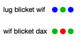
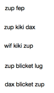
Consider the task of learning a language from a few examples

| | | | | :———————————————————-: | :———————————————————-: | :———————————————————-: |

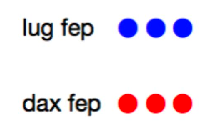As a human, you are expected to find from the above:

primitives
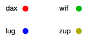
rules/function
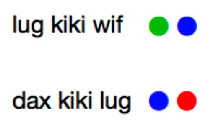
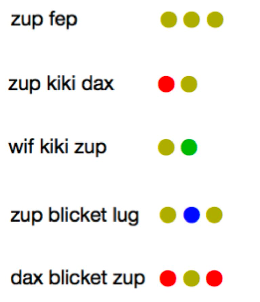
- fep - three dots
- blicket - surrounding
- kiki - after

Then we can do inference:

Query	Inference Result

note that this is meta-learning:

input data are not really “datasets”, as they have no input-label pairs. They are like data pairs chosen to reflect the task/language, hence meta-data about the language.
the output/we are learning the primitives and rules in this language. There is no directly “label” learnt.

The following section talks about how we solve this by:

Meta learning
Self-supervised meta learning
Self-supervised meta learning with a meta-grammar

Meta Learning Algorithm

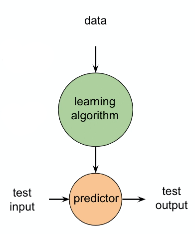
Recall that in supervised learning, we have:

where

input data $X$ and labels $Y$ being $(X,Y)\sim D$
the learning algorithm specifies the architecture we use, e.g. SVM/k-NN/CNN/etc
during training, we find parameter for the predictor
\[\theta^* = \arg\max_\theta p(\theta |D) = \arg\max_\theta p(D|\theta)p(\theta)\]
during testing/inference, we use $\theta^*$

Suppose we have some model $f_\theta$ we want to use, for example a CNN.

The goal of few-shot meta-learning is to train a model $f_\theta$ that can quickly adapt to a new task using only a few datapoints and training update iterations to $\theta$.

in other words, we want some good initialization of $\theta_0$ (learnt from other tasks as a “warm start”) such that in a new task it learns fast with only few samples

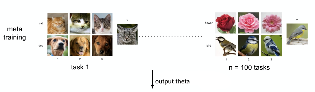
So how do we get such a handy $\theta_0$? In effect, the meta-learning problem treats entire tasks as training examples, i.e. we consider

a distribution over tasks $p(T)$ that we want our model to adapt to
for each task $T_i$ could have its own loss $\mathcal{L}_{T_i}$ and its training data distribution $q_i(x)$

Then, during meta-training (in a $K$-shot learning setting), the idea is, given a model $f_\theta$:

consider some random initialization of $\theta_0 \equiv \theta \equiv \phi$
while not done:
1. sample a batch of tasks $T_{i}$s to train from $p(T_i)$:
  1. sample a task $T_i$, e.g. compare “cat v.s. dog”
  2. draw $K$ samples from $q_i(x)$ for training, known as support set
  3. compute its loss $L_{T_i}(f_\theta)$ using the $\theta$ initialization
  4. update/see how well this initialization works by doing a few descents:
  \[\theta_i' = \theta - \alpha \nabla_\theta L_{T_i}(f_\theta)\]
  for that specific $T_i$.
2. update the initialization $\theta\equiv \phi$ as how the total loss over all tasks can be decreased if I have a better $\theta$ to begin with
  \[\theta \leftarrow \theta - \beta \nabla_\theta\sum_{T_i} L_{T_i}(f_{\theta_i'})\]
  where:
  - $f_{\theta_i’}$ is like the same model “fine-tuned” on task $T_i$.
  - $L_{T_i}(f_{\theta_i’})$ will now be evaluated on the new samples from $q_i(x)$, known as the query set to test its generalization ability as well
  - since we are taking derivative w.r.t $\theta$, and we know (if only doing a single iteration)
    \[\theta_i' = \theta - \alpha \nabla_\theta L_{T_i}(f_\theta)\]
    essentially this term include loss of losses.
output the learnt $\theta$ being the better "initialization" parameters for your model $f_\theta$ which is ready for other tasks

Hence the algorithm is

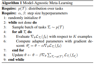
which we know is agonistic of what model $f$ we picked.

resource https://arxiv.org/pdf/1703.03400.pdf

Graphically:

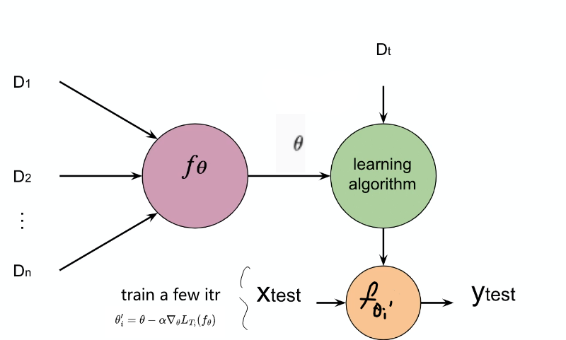
where the aim is to provide some good $\theta$ for your network $f_\theta$ such that it can get good performance on task $T_i$ with only a few updates on $\theta$.

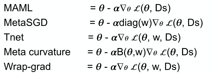
Other related meta-learning algorithms only vary in how they descent the $\theta_i’$ for each task:

Example: K-shot learning for animal classifications:

where essentially:

each task $T_i$ is classifying between two animals, i.e. a binary classification
we want to generalize well to $3$-shot $2$-way, so that our model performs well on

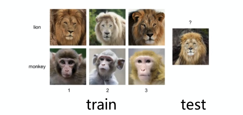
with only a few updates from $\theta$, i.e. it is almost like fine-tuning it.

Matching Network

This is essentially another approach at solving a new task $T_i$. Instead of finding a good $\theta$ for our network $f_\theta$ to start with, consider

Learning training the network $g_\theta$ to learn a good embedding network of the input such that, at test time with a new 1-shot learning task $T_i$ a simple Nearest Neighbor would work.

Specifically, consider:

learning input: all training data for all tasks at once
learning goal: learn embedding network $f_\theta, g_\theta$

where:

The key point is that when trained, Matching Networks are able to produce sensible test labels for unobserved classes without any changes to the network
reference: https://arxiv.org/pdf/1606.04080.pdf

For a simplified version, let us just say that $g_\theta = f_\theta$.

Here the idea is that we consider

\[\hat{y} = \sum_{i=1}^k a(x_q,x_i)y_i\]

which is basically a weighted sum

for $a(x_q,x_i)$ being an attention kernel. The simplest you can use is
\[a(x_q,x_i) = \text{Softmax}(c(x_q,x_i))\]
for $c(x_q,x_i)$ being a dot product
for simplicity, we assume we have $Q=1$ for training.

Then the implementations look like

BaseNetwork a backbone doing $f_\theta(x_i)$, which will be also used in Prototypical Network
the predictor then does
\[\hat{y} = \sum_{i=1}^k a(x_q,x_i)y_i\]
as specified above

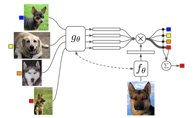
Prototypical Network

Here the idea is to consider predicting $\hat{y}$ of $x_q$ by nearest neighbor to prototypes $c_k$ of each class (learnt from the few-shot training):

\[c_ k = \frac{1}{|S_k|} \sum_{(x_i,y_i)\in S_k} f_\theta(x_i)\]

basically is saying each class $K=k$ has a prototype being its centroid. Then, for a new query $x_q$ we can simply do:

\[p(y=k|x) = \text{Softmax}(-d(f_\theta(x_q), c_k))= \frac{\exp(-d(f_\theta(x_q), c_k))}{\sum_{k'}\exp(-d(f_\theta(x_q), c_{k'}))}\]

for $-d(f_\theta(x_q), c_k)$ basically is the distance between $f_\theta(x_q)$ and $c_k$.

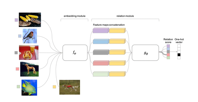
Relation Network

Instead of using Nearest Neighbor for classification, use a Neural network

Meta Learning with Meta Grammar

Instead of finding a $\theta$ as a “warm start” for the neural network $f_\theta$ on a new task, consider learning grammars.

So the general idea is:

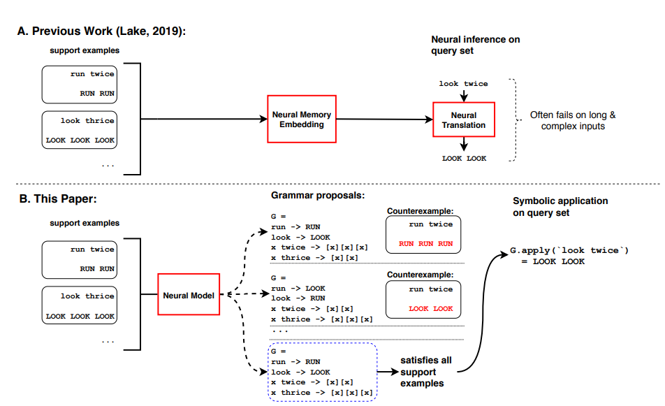
The detailed architecture looks like:

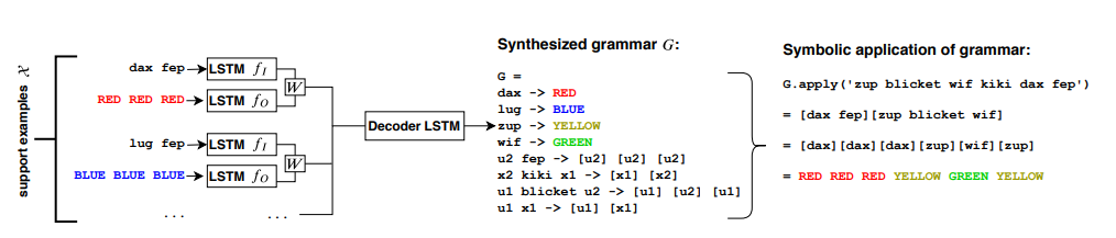
notice that essentially the entire neural model is on $p_\theta(G\vert X)$ is a distribution over grammar $G$ given the support set $X$. this works by

an encoder $\text{Enc}(\cdot)$, which encodes each support example $(x_i,y_i)$ into a vector $h_i$
\[\text{Enc}(X) = \{h_i\}^n_{i=1}\]
a decoder $\text{Dec}(\cdot)$ which decodes the grammar while attending to the support example
\[p_\theta(\cdot |X) = \text{Dec}(\{h_i\}_{i=1}^n)\]
decoder outputs a tokenized program, which is then parsed into an interpretation grammar
this is essentially the solution to the example in section Example: Learning Rule System.

Applications of DL

Applications we will dicuss include:

Deep Learning for Protein Structure Prediction
Deep Learning for Combinatorial Optimization

DL for Protein Structure Prediction

We know that proteins (a chain of amino acids) are the major building blocks of life. Structure of protein determines functions, and they are engines for your body.

There are millions of possible protein structures in nature, but only a few thousands was discovered. Hence we have the task:

given a sequence of protein, predict the structure (i.e. average of a the moving system)

e.g. predict the structure of SARS-COV-2, so that we can develop antibodies

It is very applicable since in real word, the number of sequence discovered grows faster than structures:

350M sequences
but only had recorded 170K structures

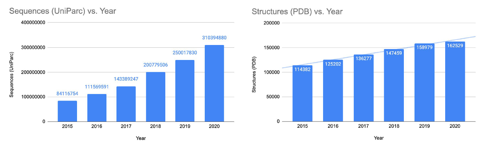
we want to fill the gap using Deep Learning.

Subtasks involved in structure prediction:

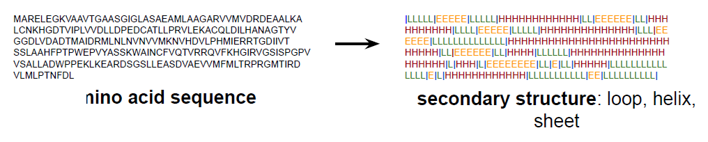
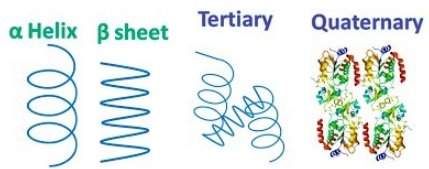
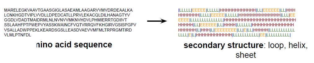
secondary structure: is this part a $\alpha$-helix, or $\beta$-sheet, or a loop, which is a labelling task

3D structure prediction: 3D position of each atom in the protein

folding: essentially the quaternary structure, how they fold when placed into a solution (liquid)

function prediction: once you have a structure, is this an enzyme? What does it do?

For Example: SARS-COV-2 protein:

SARS-CoV-2 proteins include

the Spikes, Envelope, and Membrane proteins that form the viral envelope
Nucleocapsid proteins that hold RNA (to infect other cells in your body)

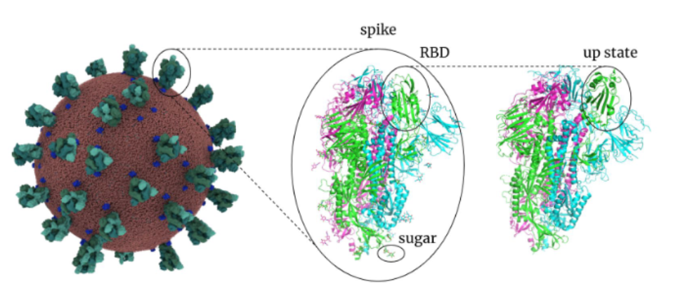
where:

the role of spike is to be able to
- use RBD (receptor binding domain) to bind to the receptor of your lung’s cell (key-lock mechanism)
- pierce through the defense and inject RNA
- hence we want to develop a drug/vaccine that can bind stronger to this than lung cells
once it gets in, the RNA gets into your cell and you are infected

Then, to predict the 3D structure of the RBD, we needed DL to generate the 3D shape.

Competitions related in this field

CASP: Critical Assessment of Techniques for Protein Structure Prediction
- Protein (3D) structure prediction
  - AlphaFold2 team won 2020 CASP14 competition
- Quality assessment, evaluation of model accuracy (EMA)
CAPRI: Critical Assessment of PRediction of Interactions
- Protein-protein interaction, protein docking
- COVID-19 Open Science Initiative
CAFA: Critical Assessment of Functional Annotation
- Protein function prediction

Secondary Structure Prediction

Here, essentially it is a Seq-2-Seq task, whether if each is a $\alpha$-helix, or $\beta$-sheet, or a loop:

Once we have this structure, it can be served as “constraints/guidelines” for 3D and quatery structure:

3D Structure Prediction

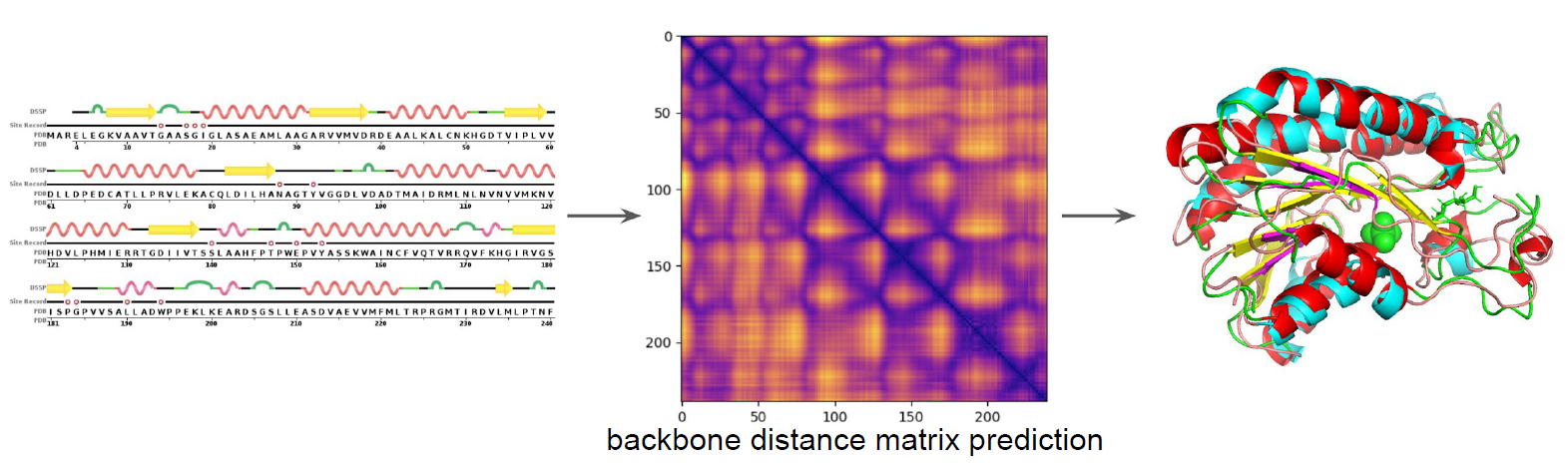
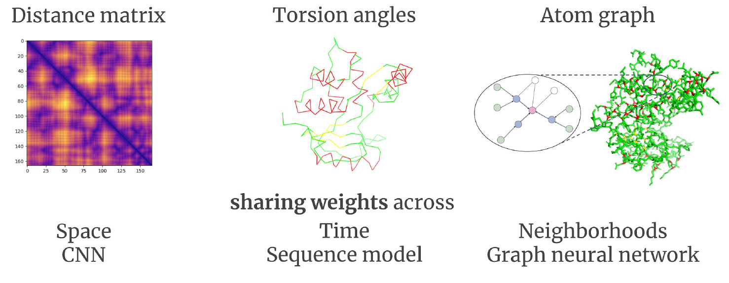
First, how do we represent the 3D structure in numbers?

One way to do it is to consider sequence of amino acids to distance matrix and torsion angles

So that essentially you want to find out:

pair-wise distance between each atom. Then we get $(n^2-n)/2$, hence $O(n^2)$
torsion angles of each particle, $O(2n)=O(n)$ since you have two angles

Then you can solve for the structure from the two above:

However, you could have also

output directly 3D position of each particle, $O(3n)=O(n)$

So why was the distance matrix useful? One use was to enable the use of Resnet to process those matrix as images:

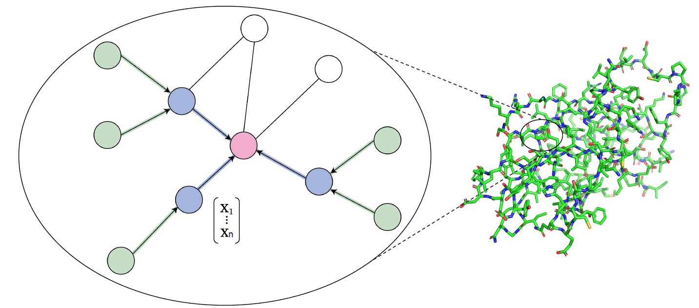
where the final atom graph is solved by:

nodes being the 3D coordinates
edges being the distance, and type of bond

Protein Structure Prediction System

The final goal is to predict the 3D structure. From the discussion above, we essentially:

find/infer the secondary structures along with other features
find/infer the torsion angles/distances
solve for 3D structure under some biological constrains

Hence the pipeline looks like

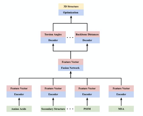
which is trained end-to-end. Notice that, alike this, it is often the case you will get many data modalities for your task (e.g. amino acids, secondary structure, etc):

then fusion network is important: allows the feature to interact in a nonlinear fashion
then the final fused representation is fed into decoders for some prediction task, e.g. predict pair-wise distance.

Predicted Structure Assessment

How do we measure the score of each prediction? In general it can be done in two ways

Model mapping from features of previous predictions to evaluation based on ground truth (RMSD, GDT_TS)
Pairwise similarity between features of different predictions

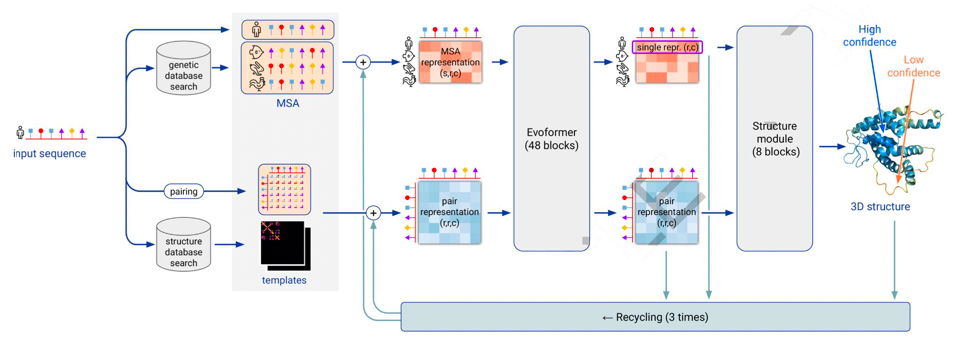
AlphaFold2

Average RMSD under 1 Angstrom

DL for Combinatorial Optimization

Combinatorial optimization is the process of searching for maxima (or minima) of an objective function $F$ whose domain is a discrete but large configuration space (as opposed to an N-dimensional continuous space). i.e. finding an optimal object from a finite/discrete set of objects.

Some simple examples of typical combinatorial optimization problems are:

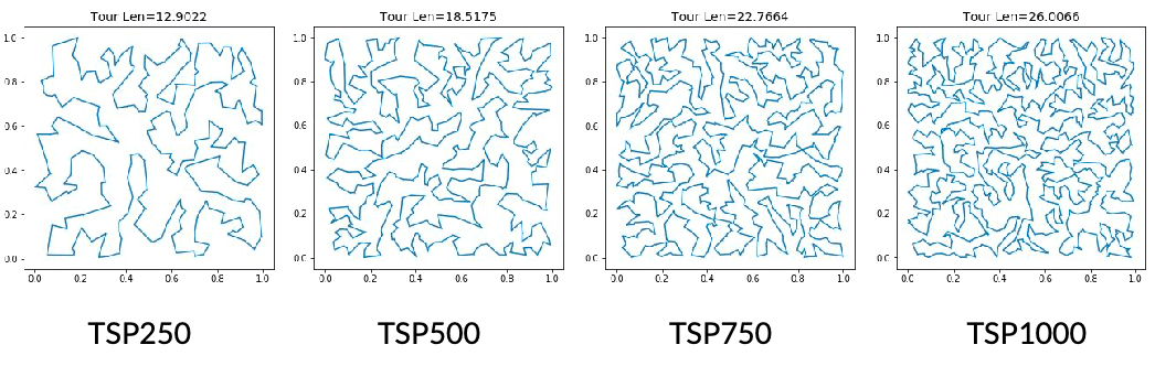
Traveling Salesman Problem: given the $(x, y)$ positions of $N$ different cities, find the shortest possible path that visits each city exactly once.

Minimum Spanning Tree: find a tree in a graph that contains the least weight (from the edges)

From a computer science perspective, combinatorial optimization seeks to improve an algorithm by using mathematical methods either to reduce the size of the set of possible solutions or to make the search itself faster.

First, some recap of typical problems:

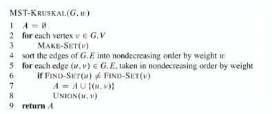
Minimum Spanning Tree: Prim, Kruskal algorithm etc. Can be solved in a polynomial time.
- Sort the graph edges with respect to their weights.
- Start adding edges to the MST from the edge with the smallest weight until the edge of the largest weight.
- Only add edges which doesn’t form a cycle , edges which connect only disconnected components (using disjoint sets)
Single Source Shorted Path: classical Dijkstra if non-negative weights. Can be solved in a polynomial time.
- Dijkstra for non-negative weights
- general SSP include Bellman-Ford
Travelling Salesman Problem: NP hard
- if we randomly distribute notes, the TSP have a strong locality, hence there are approximations that can be done in polynomial time
- a one vehicle version of VRP
Vehicle Routing Problem: What is the optimal set of routes for a fleet of $N$ vehicles to traverse in order to deliver to a given set of $M$ customers? NP hard problems

Solving MST with DL

The idea is ot represent the problem as a search tree. We already know that this problem can be solved by

But visualizing the process:

Kruskal’s Algorithm	To RL

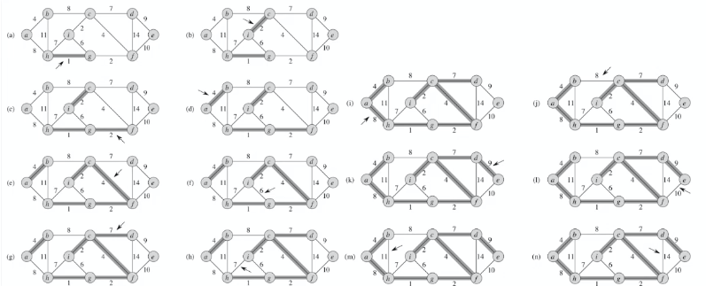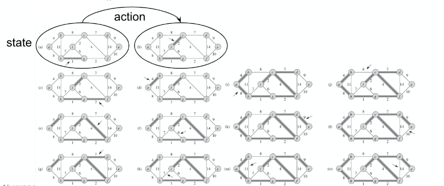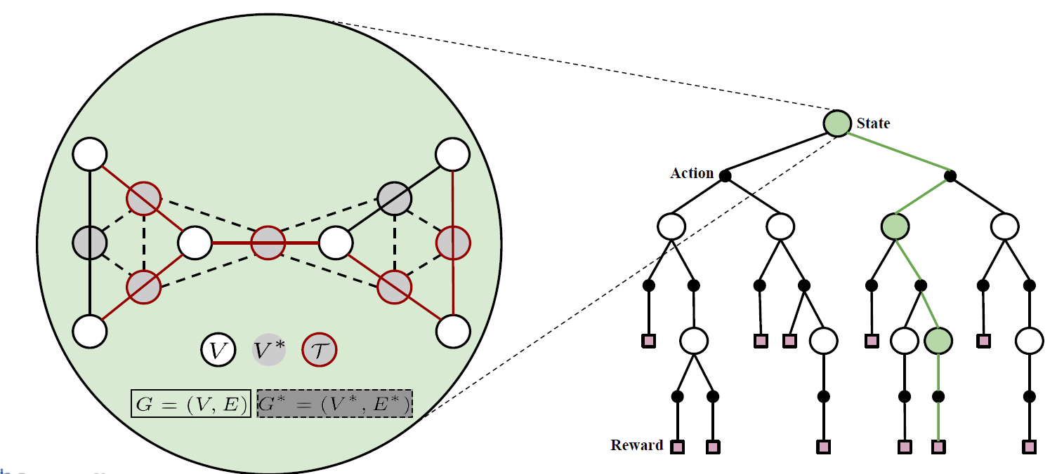
where we can represent the problem as:

state is the current graph
action is selecting one of the edges
reward: the value of the solution

Note that this action of “adding node” is general, as you can switch the representation of node/edge if your task needs to find the edges instead.

where in the above

both edges $E$ and nodes $V$ can be represented by nodes $V^*$ and $V$, respectively.

the final tree formed $T$ is highlighted in red (i.e. output of your algo)

DL Formulation of Combinatorial Optimization

Essentially you have

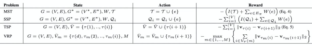
where here we separated into two types because:

the P-problems are essentially graph problems
the NP-problems are essentially becoming RL + MCTS search

DL for Autonomous Vehicles

General pippeline

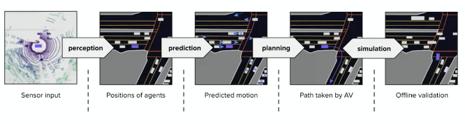
where:

for prediction, it will be a set of trajectories with probabilities
planning: is a hierarchical process depends on resolution (e.g. per second? per milisecond?)

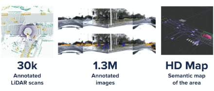
Localization and Data Collection

The ability of self-driving is unrelated to current location

though it is required for route planning, it is not relevant for driving ability
however, by just collecting what each car see, we can gain multiple perspectives and collect tons of data which we can use to reconstruct the world

Once we reconstructed the 3D model, we can obtain semantic information such as where are the lanes, traffic lights, etc:

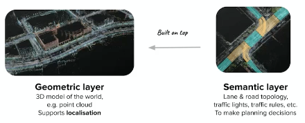
and finally this gives

Perception and Detection

Now, we have all the sensory data as our perception. How do we extract entities (e.g. bboxes of pedestrain, cars, etc)?

For instance, from video input, we might want to know where is the traffic light, other cars, etc

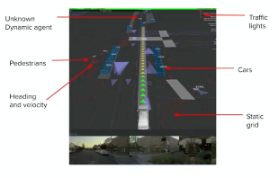
where the bottom is the input video, and the top portion is what we want.

in terms of deep learning outputs, typically we need segmentations:
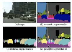
And again, as today we have tons of data from all kinds of sensors, it becomes learning from multi-modal data (e.g. from Radar, Lidar, etc, as oposed to only vision form humans)

Self-Driving Car: Prediction

Now, given the surroundings, and before I plan what I do, I also need to predict what other dynamical objects will do. i.e. I need trajectories from other dynamical objects as part of the environment as well!

therefore, we need to predict each dynamic objects we detected.
this can be estimated from current movement direction, speed, acceleration, etc

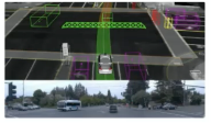
Our aim is to be able to see future trajectories of other objects, which is necessary for planning our own movement.

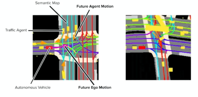
Then from all the above information, we would be able to make good plannings:

Self-Driving: Vehicle Trajectory Prediction

Essentially you need to:

given what you observe on car $A$
predict trajectories of the car (e.g. from first predicting steering angle and speed)

Predict Speed and Steering	Predict Trajectory

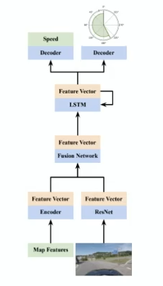though the trajectory and steering angle + speed is probably a one-to-one mapping, in reality we would use the trajectories more often as it would be detached from the make of cars, and etc.

Self-Driving Car: Planning

Now, we want to plan our high level and low level actions based on our destination:

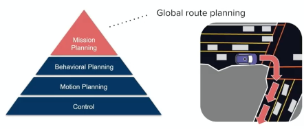
where

the high level planning basically include knowing where to go, and low level includes when to use the breaks.
Finally, this can be send to simulation where we get feedbacks without harm.

What is the “requirement” for allowing autonomous cars on road? One reasonable threshold would be having 1000 times lower probability of fatality per hour vs real world cars, i.e. we would be on average 1000 times safer!

Self-Driving: Backup

However, there are many edge cases in real life. For example, sometimes we need to follow the person guiding the traffic instead of traffic lights. Or there are other emergencies cases.

Therefore, we need a backup plan if the car does not know what to do. Currently it is done by having a tele-operator sitting in control centers, so that if something goes wrong they can opt-in.

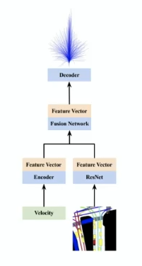
Self-Driving: Neural Network

Our end-goal is to have a car that

stay on the roard
avoid collision
head to destination

Then essentially it is a multi-task training:

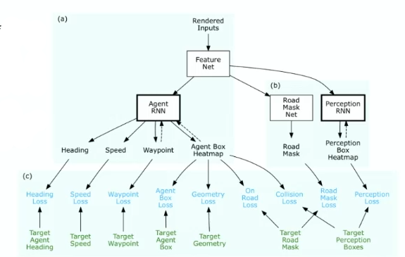
There are some paradigms:

Imitation Learning: a RL algorithm used when training data is limited
- uses environmental loss: each of the map is turned into a loss equation
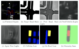
- with multiple losses, you can fuse those losses and get a set of trajectories each with some given score/probability
- but again, if anything deviates from training data (i.e. action/state not seen before), then high chance it won’t work. For instance, if some car suddenly stopped and it was not experienced in training data, then you will crash
Data Augmentation: given some training trajectory (other cars and ground truth trajectory), augment the data by perturbing the trajectory so you end up having.

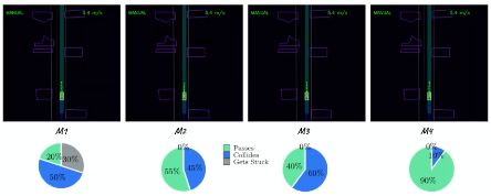
Some augmentation methods experimented and ablation studies:
- $M_1$: Imitation with past dropout
- $M_2$: $M_1$ with trajectory pertubation
- $M_3$: $M_2$ with environmental losses
- $M_4$: $M_3$ with imitation dropout (for better OOV generalization)
And the results