Reinforcement Learning

The office hours will take place by default in EE dept. student lounge, 13th FL, Mudd building. TA’s may decide to host their office hours remotely. If that is the case they will post an announcement here with a link.

TA	Day	Time
Trevor Gordon	Monday	1:30 PM - 3:30 PM
Xin Huang	Tuesday	9:30 am - 11:30 am
Jinxuan Tang	Wednesday	3:30 pm - 5:30 pm
Yukai Song	Thursday	9:30 am - 11:30 am
Gokul Srinivasan	Friday	3:30 PM - 5:30 PM

Introduction to RL

Instructors:

Chong Li (first half of the semester)
Chonggang Wang (second half)

Exam:

bi-weekly assigments 50% (first assginment out after week 2)
midterm exam 20%
final exam 30%

Key aspects of RL (as compared to other algorithms):

no supervisor, only reward signal (and/or environment to interact with)
feedback/reward could be delayed
time matters, as it is a sequenitial decision making

The general process of interaction looks like:

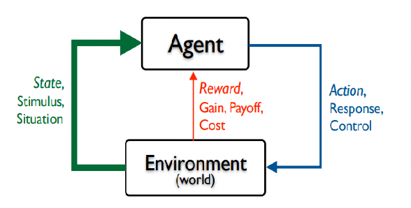
where essentially, the agent learns

a policy (e.g. the decision making agent)
\[s \in S \to \pi(a|s),a\in A(s)\]
since the action space could be dependent on the state. Note that a policy could be stochastic or determinstic
a reward indicates the desirability of that state. Reward is immediate or sometimes delayed (but as long as you have a reward for the entire episode, it is fine)
a return is a cumulative sequence of received rewards after a given time step
\[G_t = R_{t+1}+\gamma R_{t+2} + \gamma^2 R_{t+3} + ... = \sum_{k=0}^T \gamma^k R_{t+1+k}\]
where usually $\gamma < 1$ if we have infinite episodes $T \to \infty$
a value function (which depends on the policy)
\[V_\pi(s) = \mathbb{E}_\pi [G_t|S_t=s] = \mathbb{E}_\pi \left[ \sum_{k=0}^T \gamma^k R_{t+1+k} |S_t=s \right]\]
given that I am currently at $s$, what is the expected return if I follow the policy $\pi$.
a action-value function
\[Q_\pi(s,a) = \mathbb{E}_\pi [G_t|S_t=s, A_t=a] = \mathbb{E}_\pi \left[ \sum_{k=0}^T \gamma^k R_{t+1+k} |S_t=s, A_t=a\right]\]
given that I am currently as $s$, what is the expected return if I take $a$ as next step and then follow policy $\pi$. Note that if we take a “marginal” on $a$, we can get the $V_\pi$ from the $Q_\pi$:
\[V_\pi(s) = \sum_{a \in A(s)} Q_\pi(s,a) \pi(a|s)\]
which can be easily seen from their definitions. The reverse can be derived as well:
\[Q^\pi(s,a) = R(s,a)+\gamma \sum_{s' \in S}P(s'|s,a)V^\pi(s')\]
a world model (optional, so that if you know this, planning becomes much easier)
\[\mathcal{P}_{ss'}^a = \mathbb{P}[S_{t+1} = s' | S_t=s , A_t=a]\]
which is the transition probability
\[\mathcal{R}_s^a = \mathbb{E}[R_{t+1} | S_t=s,A_t=a]\]
which is the reward model. Note that it is expected when what happens next is stochastic.

The agent’s goal is to find a policy to maximize the total amount of reward it receivers over the long run.

Examples

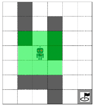
Maze

Maze Map Reward $V^{\pi^*}(s)$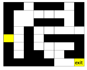

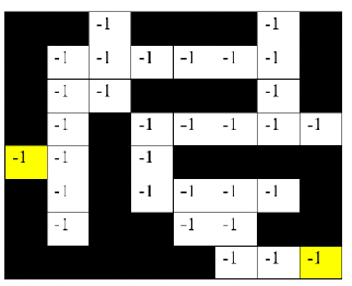
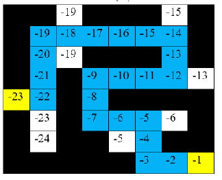
note that
- each step has a $-1$ reward (we designed, so that the agent finds the shortest path = max reward), and states is the agent’s location
- these values are computed given the optimal policy
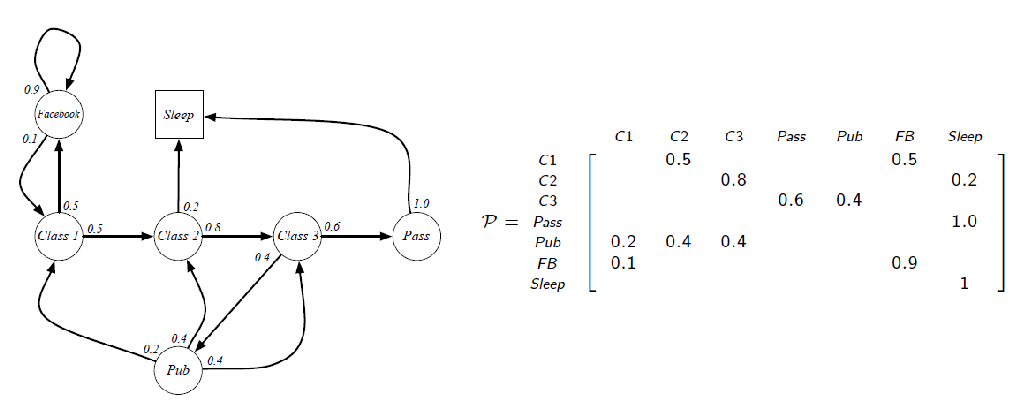
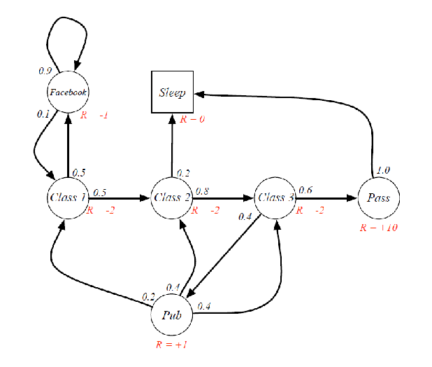
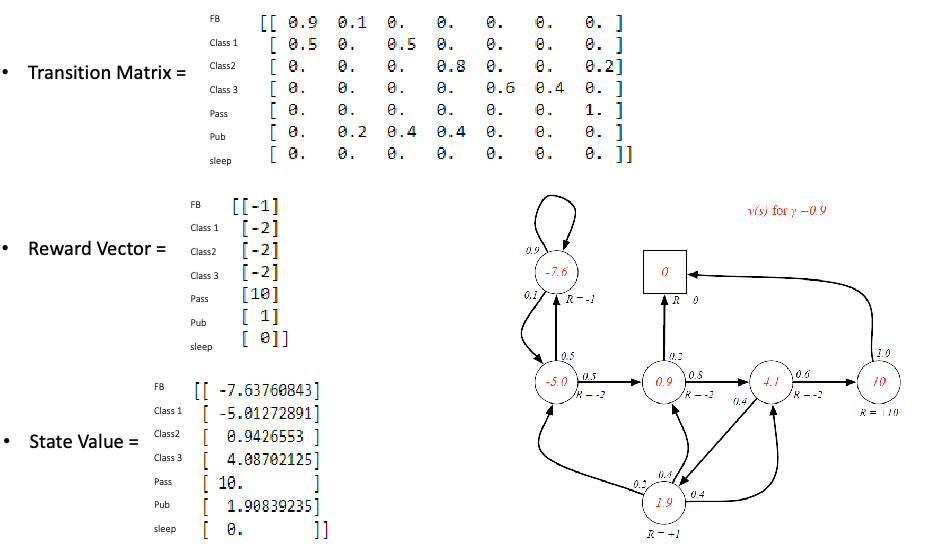
Student Markov Chain: consider some given stochastic policy:

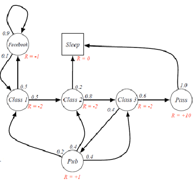
Student Markov Chain +Reward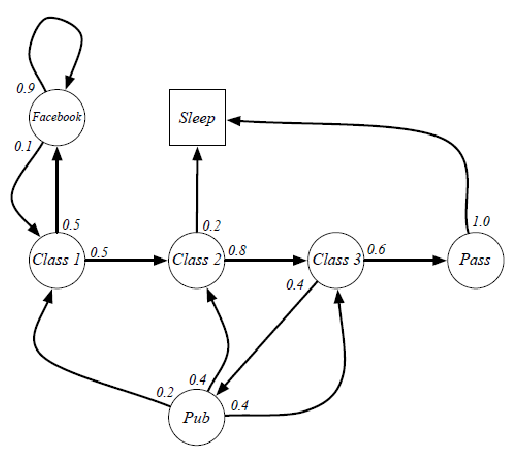

we can sample episodes for student markov chain starting from $S_1=C_1$ and obtain episodes such as:

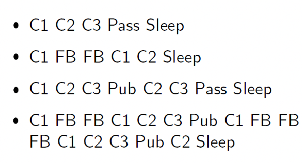
Of course, for each episode, you can have some reward given some reward model:

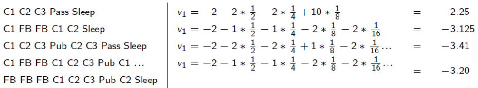
where essentially we are just computing the expected return $G_t$. But since you can have as much episodes as you want, we can consider:
\[V(S=C_1)=\mathbb{E}[G_t | S_t=C_1] = \sum_{i=1}^\infty P(\tau_i)\cdot V(\tau_i)\]
where probability of a trajectory $P(\tau_i)$ we can get since we know the transition model. However, note that this is impossible to compute since we can have infinite episodes (so we need other tricks, e.g. Bellman Equations & Dynamic Programming)

This gives rise to the definitions:

Markov Decision Process is a tuple $\lang S,A,\mathcal{P},\mathcal{R},\gamma \rang$

$\mathcal{S}$ is a finite set of states

$\mathcal{A}$ is a finite set of actions

$\mathcal{P}$ is a state trainsition probability matrix:
\[\mathcal{P}_{ss'}^a = \mathbb{P}[S_{t+1}=s'|S_t=s,A_t=a]\]

$\mathcal{R}$ is a reward function, so that $\mathcal{R}s^a = \mathbb{E}[R{t+1}\vert S_t=s, A_t=a]$ for cases when reward is not deterministic

$\gamma$ being the discount factor $\gamma \in [0,1]$.

so that if the problem can be formulated into a MDP, then we can apply RL algorithms.

And finally, after we find a policy using RL algorithm/or even train a policy using RL, we need to have access to an environment: in this course we will use OpenAI Gym. (simulation are used usually because human-invovled real environment would be too costly)

RL History

There are two threads of development

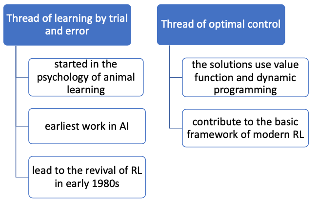
So that essentially:

control theory includes the Bellman Optimality Equations, and essentially solves the problem of how to plan, given a known model
the trial and error structure gives rise to the structure of how to train an agent to learn how to plan when we don’t know the model

Bandit Problem and MDP

Fundemental mathematical stuff behind RL algorithms.

Bandit Problem

One of the first problem that people look at. The problem is simple, but the solution shows principles in RL. The classical is the n-armed bandit problem

N-armed Bandit Problem: suppose you are facing two machines, where both are Gaussian and

reward from the first gives $\mu=5$, with variance 1

reward from the second gives $\mu=7$, with variance $1$

The obviously we will use the second machine. But in reality, the above information is not available. So what do you do? Your objective is to maximize the expected total reward over some time period.

Intuitively, the idea should be:

spend some initial money to explore and estimate the epectation using average reward
then play towards the better machine

With this, we consider $Q_t(a)$ value being the estimated value/average reward so far of action $a$ at the $t$-th play:

\[Q_t(a) = \frac{R_1 +R_2 + ... + R_{K_a}}{K_a}\]

for $K_a$ is the number of times action $a$ was chosen and $R_1,…,R_{K_a}$ being the reward associated with action $a$.

Once you estimated $Q_t(a)$, we can consider:

where we can test:

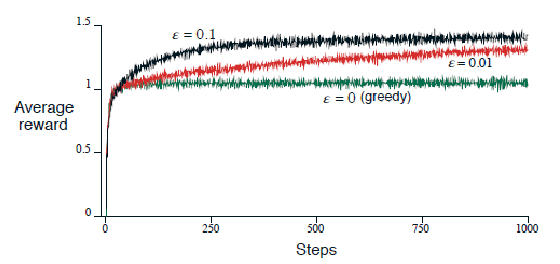
greedy policy (or $\epsilon=0$), choosing the machine with current best $Q_t(a)$
$\epsilon$-greedy means you choose a random machine with probability $\epsilon/N$ even though you know the current best. E.g. if you have, at step $t=10$, achieved $Q_{10}(a_1)=4.5,Q_{10}(a_2)=4$, then with $\epsilon=0.2$:
- choose $a_1$ with probability $0.8+0.1=0.9$
- choose $a_2$ with probability $0.1$
why is $\epsilon=0$ not good? Once you have made a unlucky estimation of the average, you may be stuck at a suboptimal solution. Especially in the early stage. But with $\epsilon$-greedy, I always have chance to jump to the correct arm.
- note that of course, there are cases where greedy policy works. But more often $\epsilon$-greedy gives more consistent performance.
but what is the optimal solution?

Exploitation vs. exploration dilemma: Should you exploit the information you’ve learned or explore new options in the hope of greater payoff?

this is what makes most RL problem hard to find the optimal

An alternative to $\epsilon$-greedy is the Softmax policy (to balance exploration and exploitation)

Softmax Policy: essentially use softmax of the Q values to give probability
\[\mathrm{Softmax}(Q(a)) = \frac{\exp(Q_t(a)/\tau)}{\sum_{a \in A} \exp(Q_t(a)/\tau)}\]
note that $\tau$ has a critical effect:

if $\tau \to \infty$, the distribution will become almost uniform

if $\tau \to 0$, then it becomes greedy action selection

But which one is better, softmax or $\epsilon$-greedy? In practice it depends on applications.

Notes on Algorithmic Implementation

do you need to store all rewards to estimate average reward $Q_k$ for each action? No, you can use a moving average
\[\begin{align} Q_{k+1} &= \frac{1}{k} \sum_{t=1}^k R_t\\ &= \frac{1}{k} \left( R_t + \sum_{i=1}^{k-1} R_i \right) \\ &= \frac{1}{k} \left( R_t + kQ_k - Q_k \right) \\ &= Q_k + \frac{1}{k}[R_k - Q_k] \end{align}\]
where $Q_k$ is for the computed average reward from the previous step, and $R_k$ is the new info. Note that this form is very commonly seen in RL:
\[\text{New Estimate} \gets \text{Old Estimate} + \alpha \underbrace{(\text{Target - Old Estimate})}_{\text{innovation term}}\]
where the innovation term would give you some idea of the new information. The step size is there because we know the innovation term will oscillate since $\mathrm{Target}$ might contain inaccuraries
what is a good step size to choose? We want your estimate, e.g. $Q$-value to converge.

an example for this to work is $\alpha=1/k$. Essentially, the intuition behind this is that it will take past information a bit more, but you should always have some non-trivial weight on the new information.
What if this is a non-stationary problem? i.e. the distribution for the n-arm bandit machine is varying over time, e.g. mean changes over time. In this case, the convergence doesn’t mean anything since the “correct” mean is moving. In this case, we can choose $\alpha$ being a constant.

Markov Decision Process

MDP formally describe an environment for reinforcement learning, where the environment is fully observable. First

Markov Property: the future is independent of the past given the present. i.e. I only care about present, past gives no information
\[P(S_{t+1}|S_t) = P(S_{t+1}|S_1,...,S_t)\]
may or may not be a good assumption in some problems. However, you can always make this a good assumption, e.g. if you choose $S_t = \text{everything up to time t}$, then this trivially holds.

A recap of the definitions

Markov Process is a tuple $\lang S,\mathcal{P}\rang$

$\mathcal{S}$ is a finite set of states

$\mathcal{P}$ is a state trainsition probability matrix:
\[\mathcal{P}_{ss'} = \mathbb{P}[S_{t+1}=s'|S_t=s]\]

An example of the transition matrix is

Markov Reward Process is a tuple $\lang S,\mathcal{P},\mathcal{R},\gamma \rang$

$\mathcal{S}$ is a finite set of states

$\mathcal{P}$ is a state trainsition probability matrix:
\[\mathcal{P}_{ss'} = \mathbb{P}[S_{t+1}=s'|S_t=s]\]

$\mathcal{R}$ is a reward function, so that $\mathcal{R}s = \mathbb{E}[R{t+1}\vert S_t=s]$ for cases when reward is not deterministic

$\gamma$ being the discount factor $\gamma \in [0,1]$. Useful for infinite episodes

For example:

Then from this, we can also define

return: think of the $R_{t+1}$ as going from a MDP to a MRP. If you start at Class 1, then you should also include $R=-2$ in your computation, just as in MDP, the reward
\[G_t = R_{t+1} + \gamma R_{t+2} += ... = \sum_{k=0}^\infty \gamma^k R_{t+k+1}\]
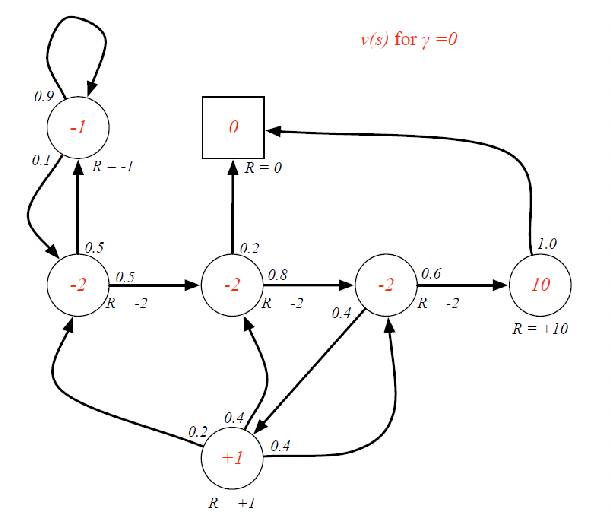
the choice of $\gamma$ affects the bahavior/goal of your algorithm
- $\gamma=0$ leads to myopic evaluation
- $\gamma=1$ leads to far-sighted evaluation

Additionally, we can also define state-value function

State Value Function (for MRP): the expected return starting from state $s$
\[V(s) = \mathbb{E}[G_t|S_t=s]\]

which we have discussed before, and to compute this intuitively would be:

start from a state $s$
compute expected reward for all possible trajectory from this state
weight it by probability of each trajectory

Which would give this

Is there an easier way than sample, weight, and sum? The Bellman Equation.

We can decompose the value function definition, and see what we get

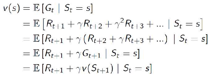
where only the last step is tricky:

what is $\mathbb{E}[\gamma G_{t+1}\vert S_t=s]$? By definition of expected value:
\[\begin{align*} \mathbb{E}[\gamma G_{t+1}|S_t=s] &= \gamma \sum_g G_{t+1} P(G_{t+1}|S_t=s)\\ &= \gamma \sum_g G_{t+1} \sum_{s'} P(G_{t+1}, S_{t+1}=s'|S_t=s)\\ &= \gamma \sum_g G_{t+1} \sum_{s'} P(G_{t+1}|S_{t+1}=s', S_t=s)P(S_{t+1}=s'|S_t=s)\\ &= \gamma \sum_{s'} \left( \sum_g G_{t+1} P(G_{t+1}|S_{t+1}=s') \right) P(S_{t+1}=s'|S_t=s)\\ &= \gamma \sum_{s'\in S}V(s') P(S_{t+1}=s'|S_t=s)\\ &= \mathbb{E}[\gamma V(s') | S_t=s] \end{align*}\]
where:
- the aim for the second equality is because we know the final result has $v(S_{t+1})$, so we need to introduce a next state $s’$.
- the third equality comes from applying chain rule for joint probability
- the fourth equality comes from the Markov Assuption, where $G_{t+1}$ does not depend on the past, only present. And that we are taking $G_{t+1}$ since it does not depend on the future state $s’$
now, given the above, we essentially realize for an ealier state:
\[\begin{align*} V(s) &= \mathbb{E}[R_{t+1}|S_t=s] + \gamma \mathbb{E}[V(S_{t+1})|S_t=s] \\ &= \mathcal{R}_s + \gamma \sum\limits_{s' \in S} \mathcal{P}_{ss'} V(s') \end{align*}\]
for $\mathcal{R}$ is the expected reward in case reward is stochastic. And in matrix form:
\[V = \mathcal{R} + \gamma \mathcal{P}V\]
for instance:

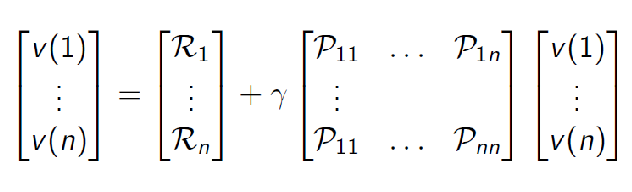
so given this, can we solve for $V$ (which is our final goal)? Simply solve it if given $P,R$:
\[\begin{align*} V &= R+\gamma P V\\ V &=(I - \gamma \mathcal{P})^{-1} R \end{align*}\]
An example using this to compute $V$ from the closed form solution:

but is this all? We have real life concerns:
- The complexity of this approach is $O(n^3)$ due to the inverse, for $n$ being the number of states
- Most often in reality you are not given $P$, i,e, you don’t know it

Two important results from the previous discussion for MRP:

Bellman’s equation for $V$:
\[V = \mathcal{R} + \gamma \mathcal{P}V\]

and we can solve for $V$ easily in closed form:
\[V =(I - \gamma \mathcal{P})^{-1} R\]

However

For large MDPs, or unknown transition models: we have the following algorithms to be our savior

Dynamic programmming (known transition, but more efficient)

Monte-Carlo evaluation (sampling, unknown transition)

Tempora-Difference learning (sampling, unknown transition)

Professor Li: “Why you need algorithm if you have the closed form solution? All algorithms are there to exchange for compute, or more oftenly, approximate a solution”.

Finally, we introduce our main problem:

Markov Decision Process is a tuple $\lang S,A,\mathcal{P},\mathcal{R},\gamma \rang$

$\mathcal{S}$ is a finite set of states

$\mathcal{A}$ is a finite set of actions

$\mathcal{P}$ is a state trainsition probability matrix:
\[\mathcal{P}_{ss'}^a = \mathbb{P}[S_{t+1}=s'|S_t=s,\textcolor{red}{A_t=a}]\]

$\mathcal{R}$ is a reward function, so that $\mathcal{R}s^a = \mathbb{E}[R{t+1}\vert S_t=s, A_t=a]$ for cases when reward is not deterministic

$\gamma$ being the discount factor $\gamma \in [0,1]$.

and remember that, most of the time, we do no have access to $P$.

Then, when given a policy $\pi(a\vert s)$, we are back to a MRP: it becomes a process of $\left\langle \mathcal{S}, \mathcal{P}^{\pi}, \mathcal{R}^{\pi}, \gamma \right\rangle$, where:

the transition matrix’s action is removed by:
\[\mathcal{P}^{\pi}_{ss'} = \sum_a \pi(a|s) \mathcal{P}_{ss'}^a\]
i.e. if I take an action $a$ at state $s$, what the the trainsition probability to $s’$? Then I take the average, to get the averae transition probability from $s\to s’$ for the policy
the reward function’s action is removed by:
\[\mathcal{R}^{\pi}_s = \sum_a \pi(a|s) \mathcal{R}_s^a\]
for $\mathcal{P}_{ss’}^{a}, R_s^{a}$ are given as part of the MDP.
when given a policy, your MDP evaluations become MRP evaluations, since now $P^\pi_{s,s’}$ is your transition matrix independent of action, and you can compute them in a closed form using our previous result.

But now, value function will depend on the policy I use, as compared to the previous cases:
\[V_\pi(s) = \mathbb{E}_\pi[G_t|S_t=s]\]
and so is the action-value function

For instance: consider a given policy $\pi(a\vert s)=0.5$ uniformly, with $\gamma=1$. Then you should get

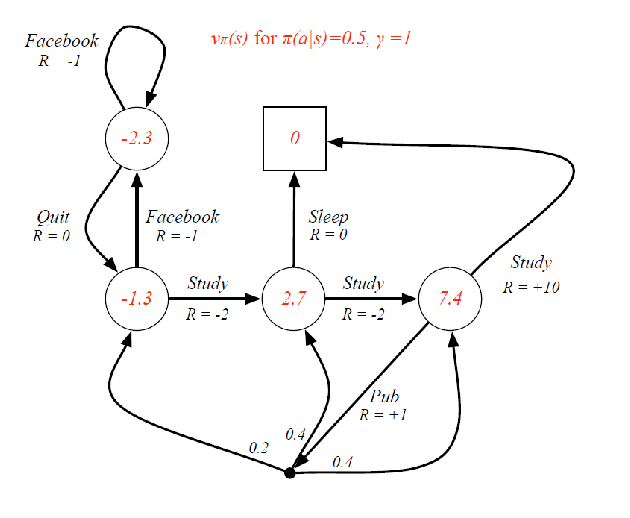
using essentially the MRP results we got, and reducing MDP given a policy to MRP.

But now, the Bellman equations depend on the policy, and we have the following:

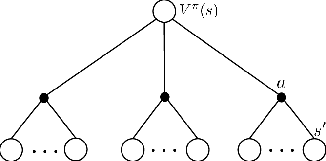
Bellman Expectation Equation: notice the connection between value function and action-value function

giving the equations for:

Value function $V_\pi(s)$ being averaging over next value functions

Action-value function $Q_\pi(s,a)$ being averaging over next action-value functions after taking action $a$ at state $s$ Hence we get:

\[V_\pi(s) = \mathbb{E}_\pi [R_{t+1} + \gamma V_\pi(S_{t+1})|S_t=s]\] \[Q_\pi(s,a) = \mathbb{E}_\pi [R_{t+1} + \gamma Q_\pi(S_{t+1},A_{t+1})|S_t=s,A_t=a]\]
or we can express them as:
\[V_\pi(s) = \sum_a \pi(a|s) Q_\pi(s,a)\] \[Q_\pi(s,a) = \mathcal{R}_s^a + \gamma \sum_{s'} \mathcal{P}_{ss'}^a V_\pi(s')\]
then using those relationships, I can express $V$ in terms of $V$, and $Q$ in terms of $Q$, which gives the Bellman Expectation Equation:
\[V_\pi(s) = \sum_a \pi(a|s) \left( \mathcal{R}_s^a + \gamma \sum_{s'} \mathcal{P}_{ss'}^a V_\pi(s') \right)\] \[Q_\pi(s,a) = \mathcal{R}_s^a + \gamma \sum_{s'} \mathcal{P}_{ss'}^a \sum_{a'} \pi(a'|s') Q_\pi(s',a')\]
which is basically the same as the equation we had with $\mathbb{E}_\pi$. Note that

when transition is deterministic given an action, then $\mathcal{P}{ss’}^a=1$ for the destined state $(s,a) \to s’$, and $\mathcal{P}{ss’}^a=0$ otherwise.

similarly, the expected reward $\mathcal{R}_s^a$ is used when reward is non-deterministic given a $s,a$,

And with this, we again have the closed form solution as implied by the above as we reduced MDP to MRP once we have a policy:

Closed Form Solution for $V^\pi$ in MDP: the Bellman’s expectation equation can essentially be translated to the MRP version:
\[V_\pi = \mathcal{R}^{\pi} + \gamma \mathcal{P}^{\pi} V_\pi\]
and the closed form solution is:
\[V_\pi = (\mathbb{I} - \gamma \mathcal{P}^{\pi})^{-1} \mathcal{R}^{\pi}\]
for $\mathcal{P}^\pi, \mathcal{R}^\pi$ being the transition and reward matrix reduced to MRP implied by the policy $\pi$.

Optimal Value Functions and Policies

Now, we understand the basics of MDP, and how we are essentially solving it by reducing to MRP, we come back to the central problem of control: how to find the *optimal* policy and/or the optimal value function?

First, we need to define what they are:

Optimal Value Function: the value function that maximizes the expected return for any given policy $\pi$:
\[V_*(s) = \max_\pi V_\pi(s)\]
and the optimal action-value function is the same:
\[Q_*(s,a) = \max_\pi Q_\pi(s,a)\]

But what about optimal policy, which if we recall are distributions $\pi(a\vert s)$? We can define it as:

Optimal Policy: we can define a partial ordering
\[\pi > \pi' \iff V_\pi(s) \geq V_{\pi'}(s),\quad \forall s\]
and note that, the two most important attribute for a problem

(existence) solution always exists. For any MDP, there eixts an optimal policy (e.g. see example below)

(uniqueness) the optimal policy not unique, but all optimal policies achieve the same value function/action-value functin.

For instance, we can give an optimal policy better than all other policies

\[\pi_*(a|s) = \begin{cases} 1 & \text{if } a=\arg\max_{a\in A} Q_*(s,a)\\ 0 & \text{otherwise} \end{cases}\]

which is optimal, meaning there always exist an optimal policy. But in reality, we don't know $Q_*$ yet. So our task remains how we can find such a policy, now that we know it exists.

Bellman Optimality Equation: we can again draw the graph, and derive the optimality equations from $V_,Q_$, which gives us some idea how we can find it

giving the equations for intuitively as:
\[V_*(s) = \max_a Q_*(s,a)\] \[Q_* (s,a) = \mathcal{R}_s^a + \gamma \sum_{s'} \mathcal{P}_{ss'}^a V_*(s')\]
and we can combine them to obtain a form only including itself:
\[V_*(s) = \max_a \left( \mathcal{R}_s^a + \gamma \sum_{s'} \mathcal{P}_{ss'}^a V_*(s') \right)\] \[Q_*(s,a) = \mathcal{R}_s^a + \gamma \sum_{s'} \mathcal{P}_{ss'}^a \max_{a'} Q_*(s',a')\]
this is essentially the basis of all RL algorithms and what they aim to solve

But now there is a $\max$, and we can no longer have a closed form solution as the equations become nonlinear. Therefore, we need to use iterative solution algorithms to approximate them (these two equations are the fundementals of the whole RL algorithm)

Value Iteration
Policy Iteration
Q-learning
SARSA
etc.

Extended MDP

Sometimes, this is not MDP by nature, but we can do some modification and convert them to MDP

Partially Obseravable MDP: for instance, the robot can only observe neighboring grids, but not the global information

therefore, technically:

I do not know $s$, but I know something related.
Solved by introducing belief MDP (see wiki for more details)

Belief MDP

ideally, we want $\pi(a\vert s)$ given a state. All I have is a history $h=(A_0,O_1,…,A_{t-1},O_t,R_t)$

therefore, we can consider a belief state (instead of state):
\[b(h) = (\mathcal{P} (S_t=s^1 | H_t = h),\mathcal{P} (S_t=s^2 | H_t = h), ...,\mathcal{P} (S_t=s^n | H_t = h) )\]
which is a probablity over all possible states.

note that we do not have to encode a belief state like this. In the case of a continous distirbutoin, this can be a gaussian distribution, for instance.

then your policy becomes:
\[\pi(a| b(h))\]
notice that belife states satisfy Markov propety

Continous State MDP: what if your state is continuous

discretization on the continous-state.
- but this becomes a trade-off between granuality = accurarcy v.s.
use a value function approximation to approximate value directly

Model-based RL

Keep in mind that all approaches is still tightly related to the bellman optimality equations

Notation: note that we try to capitial letter such as $V$ to represent the true/random variable, and $v$ represent our estimate/realization.

Introduction of Dynamic Programming

DP refers to a collection of algorithms that can be used to compute optimal policies given a perfect model of the environment as a MDP

because at each iteration, we need some form of $\mathcal{P}{ss’}^a V_k(s’)$ to update $V{k+1}$

for now, we assume a finite MDP, but DP ideas can easily be extended to cnotonus states or POMDP

However, Classical DP algorithms are of limited utility in RL. Why?

Need perfect model
Great computational expense

But regardless, if those can be overcome, we would like to perform two tasks in general:

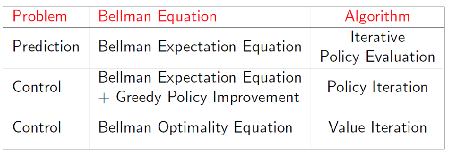
prediction: given a policy $\pi$ and the MDP, evaluate how good it is by outputting its value funciton $V_\pi$
control: given a MDP, find the optimal policy $\pi_*$

Prediction: Policy Evaluation

Aim: given any policy $\pi$, we want to evaluate its value function in a MDP.

The key idea is the Bellman equation: assuming we know everything on the RHS, then that should give me the correct value on LHS:

\[V_\pi(s) = \sum_a \pi(a|s) \left( \mathcal{R}_s^a + \gamma \sum_{s'} \mathcal{P}_{ss'}^a V_\pi(s') \right)\]

using this idea of dependency=constraint, we can iteratively estimate $V_\pi(s)$ by:

\[V_{k+1}(s) = \sum_a \pi(a|s) \left( \mathcal{R}_s^a + \gamma \sum_{s'} \mathcal{P}_{ss'}^a V_{k}(s') \right)\]

which is called a synchronous backup since it uses $V_k(s)$ even if we have for some states a better estimate $V_{k+1}(s)$

Synchronus Policy Evaluation:

Repeat until convergence:

store $V_k(s)$

for each state $s \in S$:

estimaet $V_{k+1}(s)$ by
\[V_{k+1}(s) = \sum_a \pi(a|s) \left( \mathcal{R}_s^a + \gamma \sum_{s'} \mathcal{P}_{ss'}^a V_{k}(s') \right)\]

use the latest update $V_{k} \gets V_{k+1}$

But do we always needs such an interation, as we saw in some examples in HW1?

Note that in homeworks, we had this bottom up approach where we found the correct value function in one step. For instance, we can compute the following value function of a policy:

then since $V(S=s_{t+2})=0$ for any state, we can compute $V(S=s_{t+1})$ without any error using the backup equation
\[V_\pi(s) = \sum_a \pi(a|s) \left( \mathcal{R}_s^a + \gamma \sum_{s'} \mathcal{P}_{ss'}^a V_{\pi}(s') \right)\]
and all can be done over one iteration.

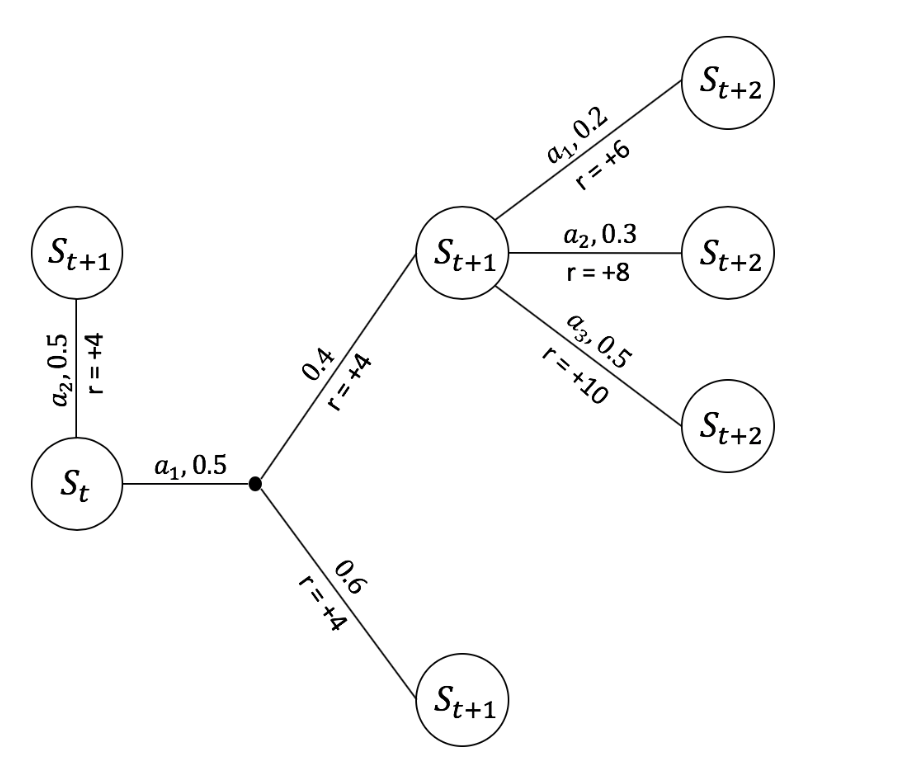
But in reality, often your state space is not a tree, i.e. to get to $S=s_{14}$ in the example below, there will be loops in your tree (i.e. you can get to $s_{14}$ from $s_{13}$, and to get to $s_{13}$ you can also start from $s_{14}$). Therefore, since then you cannot estimate $V(S=s_{14})$ correctly, you will need a loop for convergence.

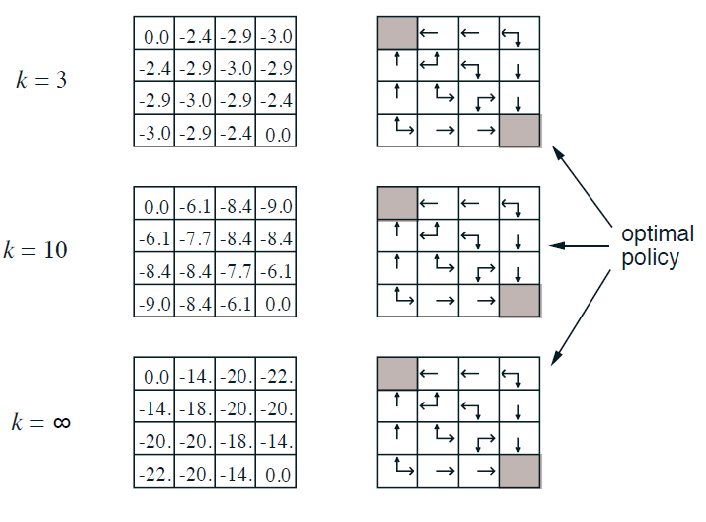
For Example: Small Grid World

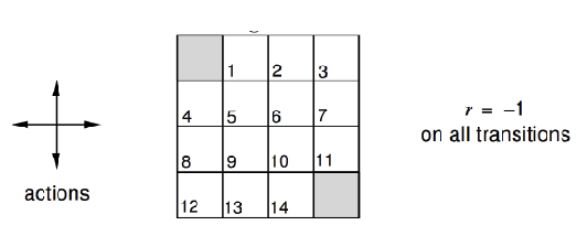
where we have:

reward of $-1$ for all non-terminal states, and there is one terminal state marked in grey
undisconuted MDP with $\gamma =1$
actions leading out of the state gives no changes (i.e. go left of $s_8$ is still $s_8$)

Question: if my policy is random $\pi(a\vert s)=0.25,\forall a$, what is the value of it/how good is this?

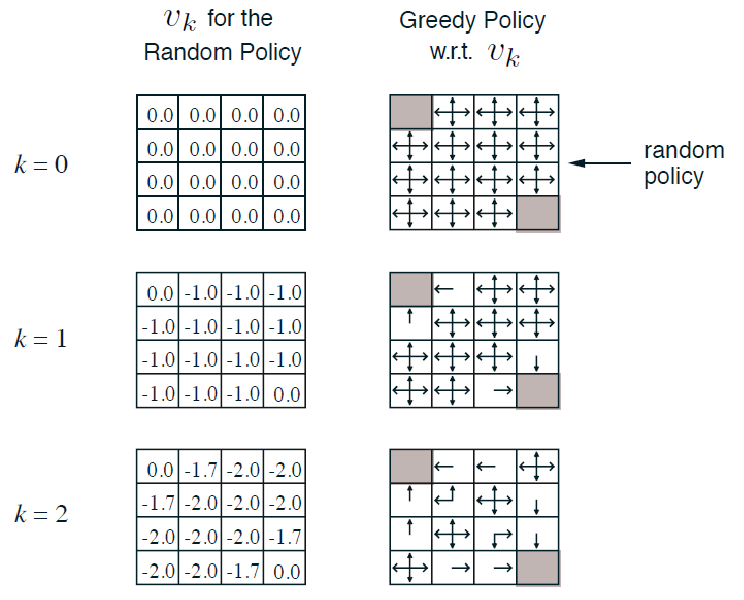
Since we also have transition model, we can use the DP algorithm. We can initialize $V_0(s)=0$:

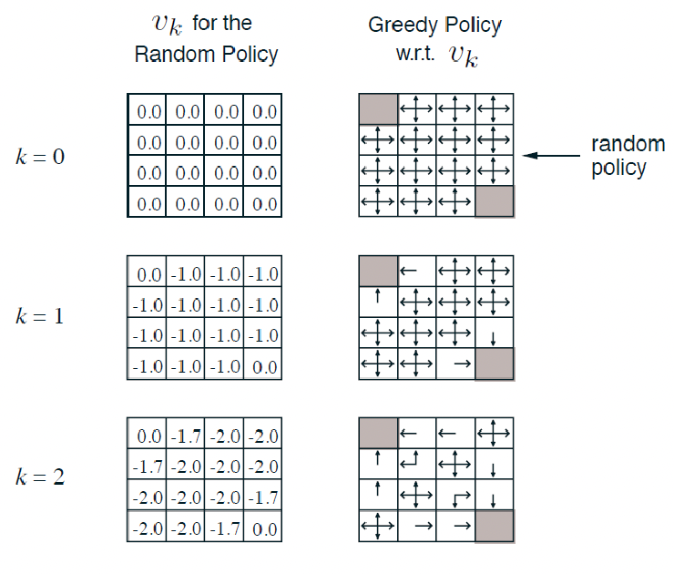
for intance, to compute $V_2(s=1)$ would be:

\[\begin{align*} V_{k=2}(s_1) &= \sum_a 0.25 \cdot \left( -1 + \gamma \sum_{s'} \mathcal{P}_{ss'}^a V_{k=1}(s') \right) \\ &= 0.25 (-1 + 0) + 0.25 (-1 + -1) + 0.25 (-1 + -1) + 0.25 (-1 + -1) \\ &= -1.75 \end{align*}\]

where all the $V_1(s)$ comes from our estimate from $v_1$ at the previous timestep.

Additional Question: what would be my control?

(This is just a lucky case that we got optimal policy in one greedy step.) We know that the value function is for a random policy, but can we get a better policy from it? Notice that by simply using the greedy policy of $\pi$:

| | | | ———————————————————— | ———————————————————— |

notice that this is essentially performing exactly one iteration of policy improvement, but we luckily get the optimal policy just by doing policy improvement once

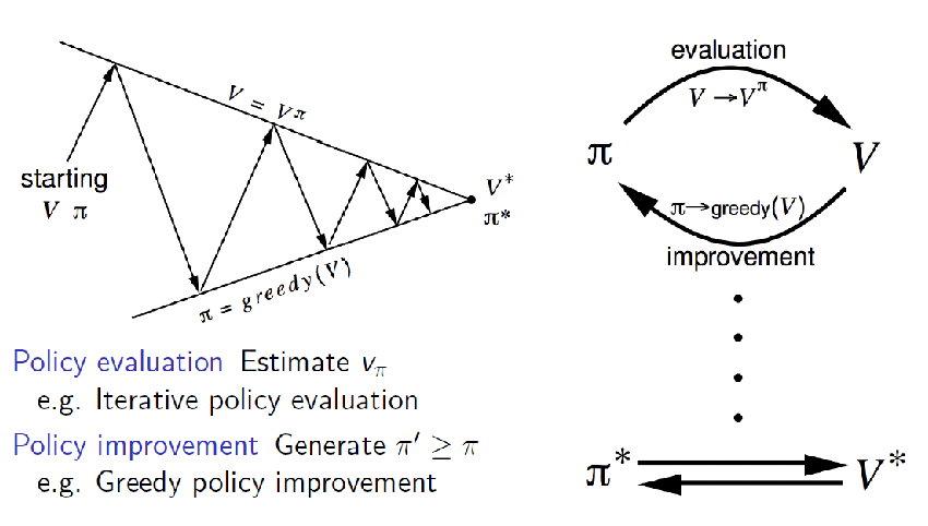
Control: Policy Improvement and Policy Interation

Now I have evaluated a policy, I would like to improve the policy and perhaps find the best policy

Policy Improvement: generate a policy $\pi’$ that is better than $\pi$

one way to guarantee improvement is to apply a greedy policy
\[\pi' = \mathrm{greedy}(V_\pi)\]
and we can later show that indeed improves the policy and is useful.

Policy Iteration: since we can get a better policy from old value, then we can iterate:

Repeat until no improvement/convergence

(Policy Evaluation) evaluate current policy $\pi$

(Policy Improvement) improve the policy (e.g. by acting greedily) by generating $\pi’ \ge \pi$

This gives the policy iteration algorithm in more details:

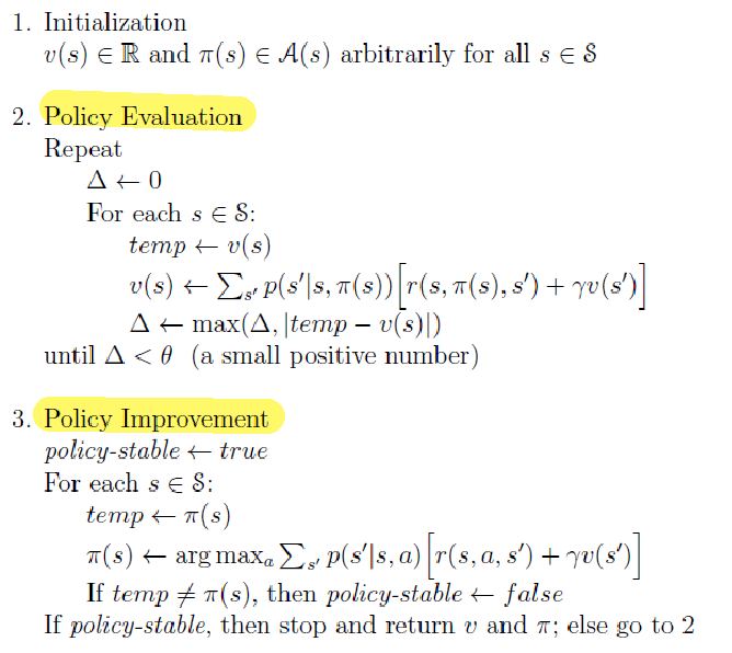
where essentially

during policy evaluation, we are taking $\Delta$ to be the largest error we encountered for each state
we are selecting the greedy policy by selecting the best action given the value function.

Proof: We want to prove that greedy policy always improve the policy, hence we have a monotonic improvement

Consider some existing deterministic policy $\pi(s)$, and we have a greedy policy version $\pi’(s)$:

\[\pi'(s) = \mathrm{greedy}(\pi(s)) = \arg\max_{a \in A}q_\pi(s,a)\]

Then by definition, the action-value must have obviously improved the policy by one-step

\[q_\pi(s,\pi'(s)) = \max_{a \in A} q_\pi(s,a) \ge q_\pi(s,\pi(s)) = v_\pi(s)\]

where the last step is due to the fact that we are using a determistic policy, so the state-value function will be the same as value function since you always only choose one action per state.

Finally, we just need to show that $V_{\pi’}(s) \ge V_\pi(s)$ by connecting the above

\[\begin{align*} v_{\pi}(s) &\le q_\pi(s,\pi'(s)) \\ &= \mathbb{E}_{(a,r,s'|s) \sim \pi'}[ \mathcal{R}_{t+1} + \gamma v_\pi(S_{t+1}) | S_t=s ] \\ &\le \mathbb{E}_{\pi'}[ \mathcal{R}_{t+1} + \gamma q_\pi(S_{t+1}, \pi'(S_{t+1})) | S_t=s ] \\ &\le \mathbb{E}_{\pi'}[ \mathcal{R}_{t+1} + \gamma R_{t+2} + \gamma^{2} q_\pi(S_{t+2}, \pi'(S_{t+2})) | S_t=s ] \\ &\le \mathbb{E}_{\pi'}[ \mathcal{R}_{t+1} + \gamma R_{t+2} + \gamma^{2} R_{t+3} + ... | S_t=s ] \\ &= v_{\pi'}(s) \end{align*}\]

where:

the second equality is because we have are sampling the immediate next step from $\pi’$, but the rest is following $\pi$.
third inequality relies on the fact that we are a deterministic policy and $q_\pi(s,\pi’(s)) \ge v_\pi(s)$ by construction

Notice that since the improvement is monotonic, then we have everything becomes an equality at convergence:

\[q_\pi(s,\pi'(s)) = \max_{a \in A} q_\pi(s,a) = q_\pi(s,\pi(s)) = v_\pi(s)\]

meaning that the Bellman optimality equation is satisfied

\[v_\pi(s) = \max_{a \in A}q_\pi(s,a)\]

which means the $\pi$ we get at the end of convergence is the optimal policy

Generalized Policy Iteration: the general recipe include:

any policy evaluation algorithm

any (proven) policy improvement

repeat until convergence to the optimal policy

But whatever new algorthim you come up with, we want to measure/compare (note that the converged value function is optimal, hence the same):

convergence speed: how fast the algorithm can converge
convergence performance: same convergence speed, but variance during training could be big/small

Control: Value Iteration

Aim: We want to improve the speed of the policy iteration algorithm because each of its iterations involves policy evaluation, which itself is an iterative computation through the state set.

Intuition, we notice that at $k=3$ in the example before, just one greedy policy we already get the optimal policy even if the value function has not converged


Therefore, maybe we can directly improve before waiting for converged value function

Value Iteration:

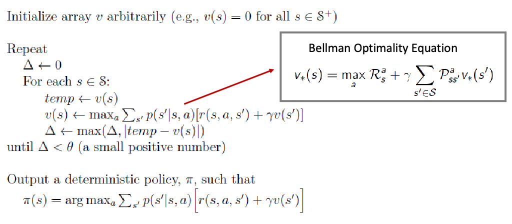
where essentially

I computed my $v(s’)$ for one round, and took the max (greedy policy) directly afterwards
notice that this is also the Bellman Optimality Equation
it is also proven that this converges to the optimal value

Value Iteration is used much more often than policy iteration due to its faster compute

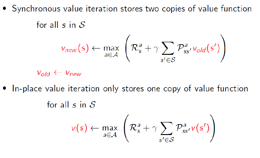
Summary: Synchronous DP

Note that all the above is synchronous DP, because at each step $k+1$ we are using the value function strictly from step $k$.

major dropback: even for value iteration, it needs to iterate through every state at each iteration (which could be intractable for large state space)
Asynchronous DP: maybe we can selectively update, or update more in real time

Asynchronous DP

Before, we compute the new value for all states at $t=k+1$ strictly using $t=k$ values, meaning for each improvement we need to wait until all states are updated.

Aim: We want to see improvement a bit faster, instead of waiting for the entire sweep of states to complete. We want our algorithm to not get locked into any hopelessly long sweep before it can make progress.

but note that this does not necessarily mean less compute

Three simple ideas in Asynchronous DP:

in-place DP
Prioritized Sweeping
Real-time Dynamic DP

In-place DP

Intuition: since we already have a new value for some states we finished computing at $t=k+1$. we use the new value directly before completing the entire estimate over all states

note that already here, we made an improvement for memory. But what about state space complexity?

Prioritized Sweeping

Intuition: instead of updating each step in a fixed order, we can consider a better order to update the states so that we can perhaps converge faster. For instance, we can use the size of the Bellman error as a guidance.

For states with large Bellman error, we might want to update them first

\[\text{Bellman Error}(s) = \left| \max_{a\in A} \left( \mathcal{R}_s^{a} + \gamma \sum\limits_{s'\in S} \mathcal{P}_{ss'}^{a} v(s') \right) - v(s)\right|\]

which is basically comparing the difference between a target the current estimate. But this means we need:

first compute this error for every state, then choose which one has the largest error to update
next, we need to update the error table, which can be done only on the affected states $s'$ (the error is only a functoin of current state and next state)
no guaranteed convergence to the optimal policy

Real-Time DP

Intuition: I only update the value function $V(s)$ on states that the agent has seen, i.e. is relevant for the agent

agent has a current policy $\pi$
agent performs some action and observe $S_t, A_t, R_{t+1}$, and is at $S_{t+1}$
backup the value function $V(S_t)$ using the new observation
\[v(S_t) \gets \max_{a\in A} \left( \mathcal{R}_{\textcolor{red}{S_t}}^{a} + \gamma \sum\limits_{s'\in S} \mathcal{P}_{\textcolor{red}{S_t}s'}^{a} v(\textcolor{red}{s'}) \right)\]
notice that this is off-policy since the value now is not about the behavior policy
update the policy $\pi$ using the new value function and repeat

Note that, again, there is no guaranteed convergence to the optimal policy

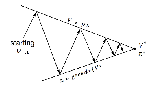
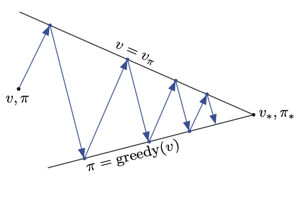
Generalized Policy Iteration

Policy iteration consists of two simultaneous, interacting processes:

one making the value function consistent with the current policy (policy evaluation)
making the policy greedy with respect to the current value function (policy improvement).

Up to now we have seen:

In policy iteration, these two processes alternate, each completing before the other begins, but this is not really necessary (e.g. value iteration).
In value iteration, for example, only a single iteration of policy evaluation is performed in between each policy improvement.
In asynchronous DP methods, the evaluation and improvement processes are interleaved at an even finer grain. In some cases a single state is updated in one process before returning to the other.

Genearalized Policy Iteration: As long as both processes (policy evaluation and policy improvement) continue to update all states, the ultimate result is typically the same—convergence to the optimal value function and an optimal policy.

Intuitively, the evaluation and improvement processes in GPI can be viewed as both competing and cooperating.

They compete in the sense that they pull in opposing directions. Making the policy greedy with respect to the value function typically makes the value function incorrect for the changed policy, and making the value function consistent with the policy typically causes that policy no longer to be greedy (i.e. has a better policy given this new value function)
In the long run, however, these two processes interact to find a single joint solution: the optimal value function and an optimal policy

Therefore, why GPI holds, i.e. usually converge to optimal value/policy, can be intuitively explained as:

The value function stabilizes only when it is consistent with the current policy,

The policy stabilizes only when it is greedy with respect to the current value function.

Thus, both processes stabilize only when a policy has been found that is greedy with respect to its own evaluation function. This implies that the Bellman optimality equation holds, and thus that the policy and the value function are optimal.

This overall idea of GPI is used in almost any RL algorithms

Model-free RL

Recall that Model-based RL requires knowing the transition function and the reward function. More importantly in a Model-Based problem:

we could get a closed form solution if the state space is small in a model-based MDP (using the Bellman’s equation)
iterative algorithms, that uses Bellman expectation equation, are used for estimating policy value
control algorithm (i.e. value iteration), that uses Bellman optimality equation, are used to find optimal value/policy

But more often in reality we don't know the model. So how do we solve the control problem?

Aim: we can use sampling to estimate the missing transition/reward models. The key question is then how do we take samples to make our model more efficient in estimating the value functions?

MC Methods

TD Methods

Monte Carlo Learning

MC Sampling: learns from complete episodes (hence finite episodes)

hence can be only used with episodic MDP

the main idea is to consider value function of a state = mean return from it
\[V(s) = \mathbb{E}[G(s)] \approx \frac{1}{n}\sum_{i=1}^n G(s)\]

Specifically, we consider the goal of learning $V_\pi$ from episodes of a policy $\pi$

\[(S_1, A_1, R_1, ..., S_k) \sim \pi\]

is one episode from $\pi$. We ca sample many episodes, and for each episode:

compute the total discounted reward for the future for each state:
\[G_t^i = R_{t+1}^i + \gamma R_{t+2}^i + ... + \gamma ^{T-1} R_T^i\]
for $i$-th episode
estimate the value function using the law of large numbers:
\[v_\pi(s) = \mathbb{E}_\pi[G_t | S_t=s] = \lim_{n \to \infty} \frac{1}{n}\sum_{i=1}^n G^i_t(s)\]
for $G_t^i(s)$ means the discounted reward starting from state $s_t$ at the $i$-th episode

While this is the basic idea, there are many modifications of this:

every visit v.s. first visit MC estimate to have different convergence speed - bias tradeoff

collecting all episodes and computing together is computationally expensive, hence there are iterative version of this

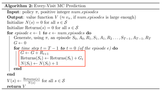
First/Every Visit MC Policy Evaluation

Consider the following two epsiodes we have sampled following policy $\pi$:

\[(S_1, S_2, S_1, S_2, S_4, S_5) \sim \pi \\ (S_1, S_2, S_2, S_4, S_5, S_3) \sim \pi\]

with some reward for each state, but ignored here. Suppose I want to estimate $V(s_1)$ from the two samples

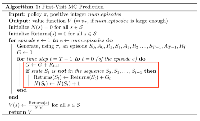
First Visit MC Policy Evaluation: to evaluate $V_\pi(s)$ for a state $s$

only for the first time step $t$ that the state is visited in an episode

count that as a sample for state $s$ and increment counter $N(s) \gets N(s) + 1$

increment total return for that state $S(s) \gets S(s) + G_t$

Then the value estimate is:
\[v_\pi(s) = \frac{S(s)}{N(s)}\]
and by law of large numbers, $N(s) \to \infty$ we have $v_\pi(s) \to V_\pi(s)$. Hence this is a consistent estimator.

Therefore, using first visit MC policy evaluation in the previous example, we would have:

\[v_\pi(s_1) = \frac{G^{1}_1(s_1) + G^{2}_1(s_1)}{2}\]

where $G^{i}_t(s)$ is the t-th timestep in the i-th episode.

Every Visit MC Policy Evaluation: to evaluate $V_\pi(s)$ for a state $s$

for the every time step $t$ that the state is visited in an episode

count that as a sample for state $s$ and increment counter $N(s) \gets N(s) + 1$

increment total return for that state $S(s) \gets S(s) + G_t$

Then the value estimate is:
\[V(s) = \frac{S(s)}{N(s)}\]
and this again, by law of large numbers, this is a consistent estimator.

Using every visit MC policy evaluation in the previous example, we would have:

\[V(s_2) = \frac{G^{1}_2(s_2) + G^1_4(s_2) + G^{1}_2(s_2) + G^{1}_2(s_2)}{4}\]

Essentially we treat every sample of even the same episode separately

Property	First Visit	Every Visit
Consistent	Yes	Yes
Biased	No	Yes
Convergence Speed	Slow	Fast

where:

usually every-visit has a faster convergence speed (unless in cases when state is rare in both cases, could have similar speed)
recall that for law of large number, we required independence of samples. However, samples from every visit are correlated. Therefore, this could be biased even though it could converge due to large number of samples.

Recall that Bias and different from Consistent:

Consistent estimator: as the sample size increases, the estimates (produced by the estimator) “converge” to the true value

Unbiased estimator: if I feed in different sample sets, the average of the estimates should be the true value

Last but not least, implementation wise since we are computing a mean, we could use recursive mean computations:

\[\begin{align*} \mu_k &= \frac{1}{k} \sum_{i=1}^k x_i \\ &= \frac{1}{k} \left( \sum_{i=1}^{k-1} x_i + x_k \right) \\ &= \frac{1}{k} \left( (k-1) \mu_{k-1} + x_k \right)\\ &= u_{k-1} + \frac{1}{k}(x_k - \mu_{k-1}) \end{align*}\]

in our case, $\mu$ would be the mean hence estimation of value $V_\pi$. This gives use the usually programmatic recursive MC updates, where we perform updates on the fly when doing sampling:

\[\begin{align*} N(S_t) &\gets N(S_t) + 1\\ V(S_t) &\gets V(S_t) + \frac{1}{N(S_t)}(G_t - V(S_t)) \end{align*}\]

whenever an update is needed. This gives a brief outline of the pseudo-code for both algorithm:

First-Visit	Every-Visit

MC for Non-Stationary State

However, if you have a non-stationary problem (e.g. mean of a distribution is time-dependent), then we want to have a dynamic estimator and we don’t want convergence.

Hence we just want to use new information directly, without doing the averaging:

\[V(s_t) \gets V(s_t) + \alpha (G_t - V(s_t))\]

which you can just convert to the equation of moving average

\[V(s_t) \gets (1-\alpha) V(s_t) + \alpha G_t\]

for a constant step size $\alpha$. We can intuitively see the difference as the previous form of $V(S_t) \gets V(S_t) + \frac{1}{N(S_t)}(G_t - V(S_t))$ since now this is a constant step size:

\[\begin{align*} V_{t+1} &= V(s_t) + \alpha (G_t - V(s_t)) \\ &= \alpha G_t + (1-\alpha) V_t \\ &= \alpha G_t + (1-\alpha) [ \alpha G_{t-1} + (1-\alpha)V_{t-1}]\\ &= \alpha G_t + (1-\alpha) \alpha G_{t-1} + (1-\alpha)^2 V_{t-1}\\ &= ... \end{align*}\]

so eventually you reach $G_1$, hence we get:

\[v_{t+1}(s) = (1-\alpha)^t v_1(s) + \sum_{i=1}^t \alpha (1-\alpha)^{t-i}G_i\]

meaning that for large $t$:

the first term will become extremely small, meaning that the old information would matter very slightly (whereas in $V(S_t) \gets V(S_t) + \frac{1}{N(S_t)}(G_t - V(S_t))$ every sample has equal contribution)
usually we want to put more weight on new information, as this is non-stationary.
but we usually use the other formula $V(s_t) \gets V(s_t) + \alpha (G_t - V(s_t))$ for update as that is more computationally efficient

But in principle, all the MC backups essentially does:

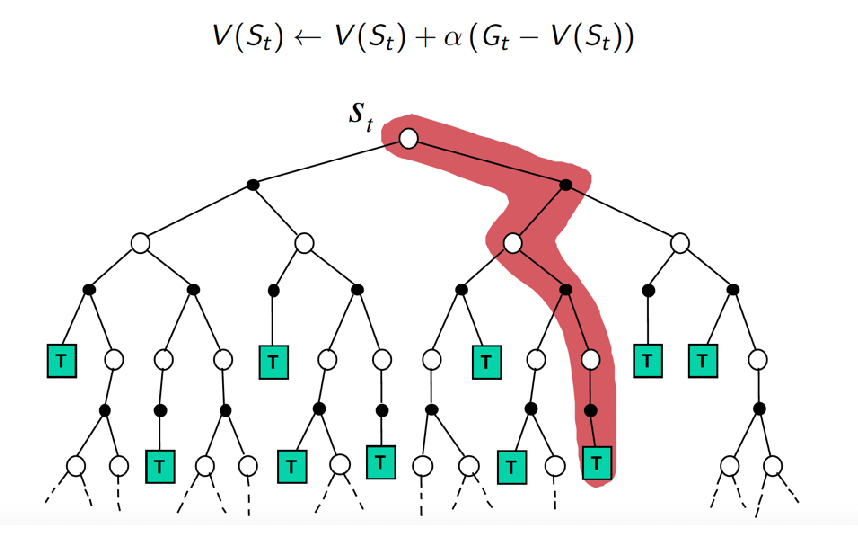
which is like a DFS when sampling. This is later constrasted with TD approaches.

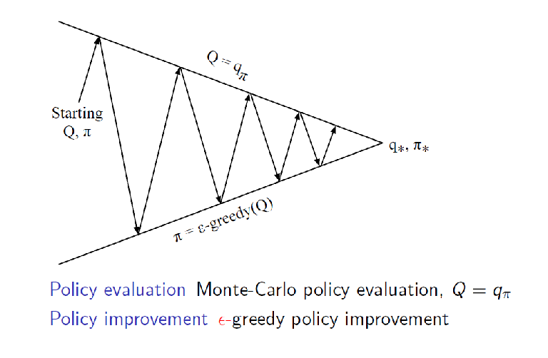
Monte Carlo Control

First, we revisit our previous approach of generalized policy iteration

where we used greedy policy for improvement and is proven to work.

Therefore, a simple idea of model-free policy improvements

use MC policy evaluation
use greedy policy improvement?

We realize that using greedy-policy here have two concerns:

if we estimateed $v_\pi$, then since greedy needs:
\[\pi'(s) = \arg\max_{a \in A} Q(s,a)\]
but if we only have $V_\pi$, then we need to compute:
\[\pi'(s) = \arg\max_{a \in A} \mathcal{R}_s^{a}+ \mathcal{P}_{ss'}^{a}V'_\pi\]
but we don’t know $\mathcal{P}$
could get me stuck in some suboptimal action due to exploitation

To solve the first problem, it is easy: we can instead use MC methods to directly estimate $Q(s,a)$

But then second problem is a little more complicated:

We can use $\epsilon$-greedy policy instead of greedy policy to allow for exploration since we are estimating the world (hence do no have complete information as in the Model-based case)
\[\pi(a|s) = \begin{cases} (\epsilon / m) + 1 - \epsilon & \text{if } a = \arg\max_{a \in A} Q(s,a) \\ \epsilon / m & \text{otherwise} \end{cases}\]
for $m = \vert A\vert$. But does this guarantee the improvement of the policy? This is proven to be true!

Proof: for all states, any Ɛ-greedy policy 𝜋, the Ɛ-greedy policy 𝜋’ with respect to is an improvement, that is,

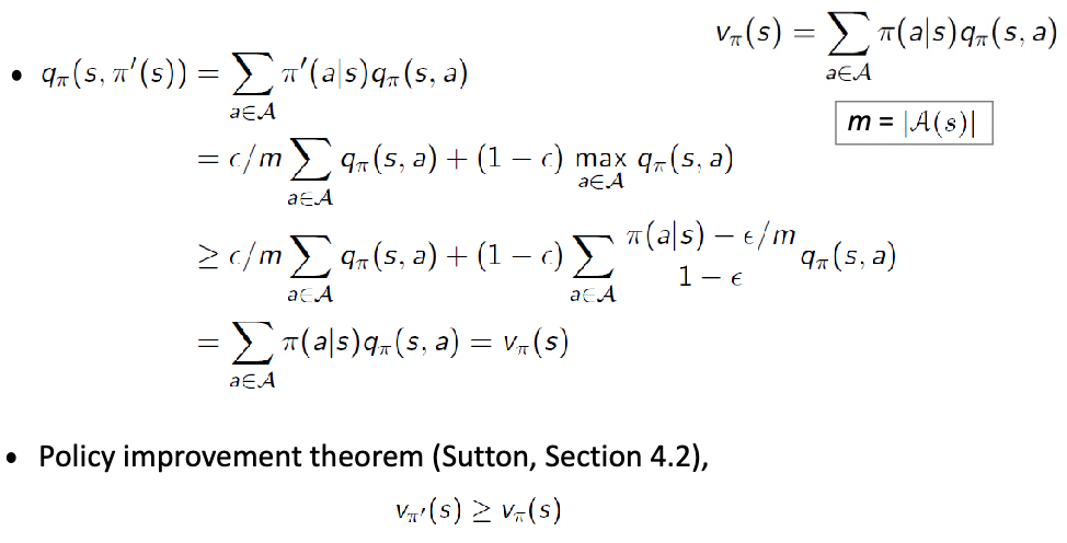
where a key step is shown above. There we wanted to show that $q_\pi(s,\pi’(s))$ is better than the old $v_\pi(s)$

the second equality comes from the fact that best action has an additional $(1-\epsilon)$ probability
the third equality comes from the fact that $\sum_x \alpha(x)f(x) \le \max_x f(x)$ for $\sum \alpha(x) = 1$. In other words, weighted average is always less than the maximum value.
the fourth equality comes from expanding the second term and cancelling the first term, with only $\sum \pi(a\vert s) q_\pi(s,a)$ left

Then finally the last step to show $v_{\pi’}(s) \ge v_\pi(s)$ which we ignored basically comes from expanding the definition of value function, and substituting in our result above.

Therefore, the final MC policy iteration becomes

Note that different from the model-based case, we cannot perform value-iteration here to simplify the computation. This is because we don’t have the transition model $\mathcal{P}$ as required in the Bellman optimality equation:
\[Q_*(s,a) = \mathcal{R}_s^a + \sum_{s'} \mathcal{P}_{ss'}^a \max_{a'} Q_*(s',a')\]

Greedy in the Limit with Infinite Exploration

Recall that we know, for every MDP problem, there exists an optimal deterministic policy by taking the greedy policy of an optimal Q-function. But if we are doing $\epsilon$-greedy, then we are not guaranteed to converge to the optimal policy.

GLIE: A learning policy is called GLIE (Greedy in the Limit with Infinite Exploration) if it satisfies the following two properties:

If a state is visited infinitely often, then each action in that state is chosen infinitely often (with probability 1):

\[\lim_{k \to \infty} N_k(s,a) = \infty\]

In the limit (as $t \to \infty$), the learning policy is greedy with respect to the learned Q-function (with probability 1):

\[\lim_{k \to \infty} \pi_k(a|s) = 1(a = \arg\max_{a' \in A} Q_k(s,a'))\]

Therefore, taking into account our policy improvement with $\epsilon$-greedy, we can still achieve optimal policy by satisfying the GLIE condition with:

\[\epsilon_{k} = \frac{1}{k}\]

for the $k$ th iteration we have updated the policy.

Therefore, we get essentially a change for policy improvement step:

\[\text{Policy Improvement:}\quad \epsilon \gets \frac{1}{k}, \quad \pi'(s) \gets \epsilon\text{-greedy}(Q)\]

Off-Policy Evaluation

So far, all we have learned is on-policy, i.e. the behavior policy used to collect samples is the same as the policy you are estimating $V_\pi$

Off-policy evaluation: means the behavior policy $\mu$ you used to collect data is not the same policy you want to estimate $V_\pi$. So you want to learn policy $\pi$ from $\mu$.

for here, we can suppose both $\mu$ and $\pi$ policy are known

essentially you may want to evaluate your $V_\pi$ or $Q(S_t,A_t)$ but only using data from $\mu$.

How do we do that? The basic methods here is importance sampling.

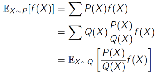
Importance Sampling

Importance Sampling: goal is to estimate the expected value of a function $f(x)$ (i.e. $G(s)$) under some probability distribution $p(x)$, without sampling from the distribution $p(x)$ but using $f(x)$ sampled from $q(x)$:
\[\mathbb{E}_{x \sim p(x)}[f(x)] =?\]
with data sampled from $x \sim q(x)$. It turns out we can easily show that, under few assumptions:
\[\mathbb{E}_{x \sim p(x)}[f(x)] = \mathbb{E}_{x \sim q(x)}\left[\frac{p(x)}{q(x)}f(x)\right]\]

Notice that the stationary distribution of states will be different, i.e. we will be considering

So, if we have samples generated from $x \sim q$, and since in our case we consider $f(X) = G_t(s)$, then basically need to consider, for each trajectory $\tau_j$ and its discounted reward $G^{j}$:

\[Q_{\tau \sim \pi}(s,a) = \mathbb{E}_{\tau \sim \mu(x)}\left[\frac{P_\pi(\tau)}{P_\mu(\tau)}G^{j}\right]\]

But what is this ratio of probability?

\[P_\pi(\tau) = P_\pi(S_t, A_t, ..., S_T, A_T)\\ P_\mu(\tau) = P_\mu(S_t, A_t, ..., S_T, A_T)\]

we can essentially use chain rule to represent this as quantities we know:

\[\begin{align*} P_\pi(\tau) &= P_\pi(S_t, A_t, ..., S_T, A_T)\\ &= \pi(A_T | S_t, S_{T-1},A_{T-1}, ..., S_t,A_t) P_\pi(S_t, A_t, S_{t+1},A_{t+1},...S_T, A_T)\\ &= \pi(A_T | S_T) P_\pi(S_T | S_{T-1},A_{T-1},...S_t, A_t)P_\pi(S_{T-1},A_{T-1},...S_t, A_t)\\ &= \underbrace{\pi(A_T | S_T)}_{\mathrm{policy} } \underbrace{P_\pi(S_T | S_{T-1}, A_{t-1})}_{\text{transition model} } P_\pi(S_t, A_t, S_{t+1},A_{t+1},...S_{T-1},A_{T-1})\\ &= ...\\ &= p(S_{1}) \prod_{i=1}^{T}\underbrace{\pi(A_{i}|S_{i})}_{\mathrm{policy}} \underbrace{p(R_{i}|S_{i},A_{i})}_{\text{reward model}} \underbrace{p(S_{i+1}|S_{i},A_{i})}_{\text{transition model}} \end{align*}\]

where

the third and fourth equality comes from the fact that we are MDP, hence future only depends on current
finally, the transition probability and reward probability will be cancelled when we do the ratio:
\[\frac{P_\pi(\tau)}{P_\mu(\tau)} = \frac{p(S_{1}) \prod_{i=1}^{T}\pi(A_{i}|S_{i}) p(R_{i}|S_{i},A_{i}) p(S_{i+1}|S_{i},A_{i})}{p(S_{1}) \prod_{i=1}^{T}\mu(A_{i}|S_{i}) p(R_{i}|S_{i},A_{i}) p(S_{i+1}|S_{i},A_{i})} = \prod_{i=1}^{T}\frac{\pi(A_{i}|S_{i})}{\mu(A_{i}|S_{i})} \equiv w_{\mathrm{IS}}\]
is called the importance sampling weight for each trajectory
can estimate any other policy, but given that we have the same coverage. unseen action in policy $\mu$, it has prob zero

Ordinary IS: the above essentially gives the ordinary IS algorithm:
\[\begin{align*} V_{\pi}(s) & \approx \frac{1}{n} \sum\limits_{j=1}^{n} \frac{p_\pi(T_j|s)}{p_\mu(T_j|s)} G(T_j)\\ &= \frac{1}{n} \sum\limits_{j=1}^{n} \left(\prod_{i=1}^{T} \frac{\pi(a_{j,i}|s_{j,i})}{\mu(a_{j,i}|s_{j,i})} \right) G(T_j)\\ &= \frac{1}{n} \sum\limits_{j=1}^{n} w_{\mathrm{IS}} \cdot G(T_j) \end{align*}\]
for practically, we are just swapping out $G(T_j)$ with $w_{\mathrm{IS}} \cdot G(T_j)$ in our previous on-policy algorithms.

Now, what are the assumptions used to make IS work? You might notice the term $\frac{\pi(a_{j,i}\vert s_{j,i})}{\mu(a_{j,i}\vert s_{j,i})}$ could have gone badly, and it is exactly the case

Importance Sampling Assumptions: since we are reweighing samples from $\mu$, if we have distributions that are non-overlapping, then this will obviously not work.

in particular, if we have any single case that $\mu(a\vert s)=0$ but $\pi(a\vert s)>0$, then this will not work.

therefore, for this to work, we want to have a large coverage: so that for $\forall a,s$ such that $\pi(a\vert s)>0$, you want $\mu(a\vert s)>0$.

Intuitively, this means that if $\pi$ is not too far off from $\mu$, then the importance sampling would work reasonably.

In practice, there are still some problems with this, and hence some variants include:

Discounting-aware Importance Sampling: suppose you have $\gamma =0$ and you have for long episodes. Then techinically since $\gamma=0$, your return is determined since $S_0,A_0,R_0$ and multiplying the weight by $w_{\mathrm{IS}}$ contributes significantly to variance
Per-decision Importance Sampling: which applies a weight to each single reward $R_T$ within the $G$.

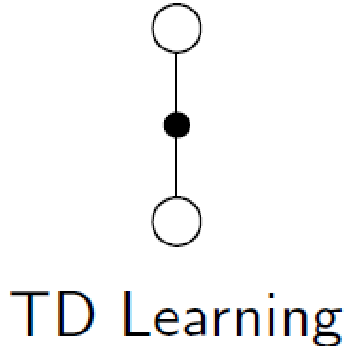
TD Learning

In practice, the MC is used much less because:

we need to wait until the agent reaches the terminal state to compute $G_t$, which is our target for update equation
- e.g. if we play go game, it needs to wait until the end of the game
hence also requires finite episode settings
large variance, because the episode can be long

Aim: TD learning tries to resolve that issue by “estimating the future” instead of waiting and using the true future. So the questions become: is there some useful information we can do without this wait?

learns from incomptele episodes, hence bootstrapping

but because you are updating from your estimate based on your estimate, there will be bias (MC has no bias)

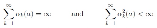
For any fixed policy $\pi$, TD(0) has been proved to converge to $v_\pi$, in the mean for a constant step-size parameter if it is sufficiently small, and with probability $1$ if the step-size prameter decreases according to the usual stochastic approximation condition:
\[\sum_{n=1}^\infty \alpha_n(t) = \infty,\quad \text{and}\quad \sum_{n=1}^\infty \alpha^2_n(t) < \infty\]
The first condition is required to guarantee that the steps are large enough to eventually overcome any initial conditions or random fluctuations. The second condition guarantees that eventually the steps become small enough to assure convergence.

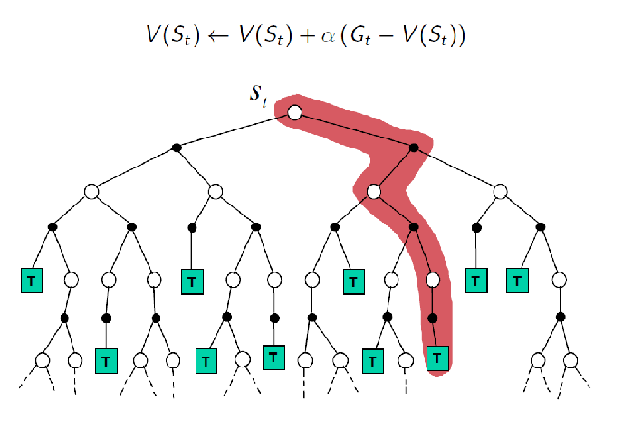
Recall that MC updates in general looks like

\[V(S_t) \gets V(S_t) + \alpha (\underbrace{G_t}_{\text{MC target}} - V(S_t))\]

which is the actual return, but in TD(0) we can update using an estimated return

\[V(S_t) \gets V(S_t) + \alpha (\underbrace{(R_{t+1} + \gamma V(S_{t+1})}_{\text{TD(0) target}}) - V(S_t))so that :\]

essentially I am utilizing the fact that:
\[G_t = R_{t+1} + \gamma R_{t+2}+ \gamma ^2 R_{t+3}+ ...= R_{t+1} + \gamma V(S_{t+1})\]
hence since we can approximate $V(S_{t+1}) \approx v(s_{t+1})$, we get our TD(0) update
intuitively, this TD(0) means that I wanted to make update on $S_t$ and I do this by:
- taking an action $A_t$ and get to $S_{t+1}$
- then using my trajectory $S_{t}, R_{t+1}, S_{t+1}$ to update by estimating the expected return I would get in the future
so this means that like MC, I will still be estimating with acting and sampling experience from real environment

But since TD$(0)$ is only moving/looking one step forward at $V(S_{t+1})$, you can easily also look many steps:

General TD$(n)$ updates: since we can also have
\[G_t = R_{t+1} + \gamma R_{t+2}+ \gamma ^2 R_{t+3}+ ...= R_{t+1} + \gamma R_{t+2}+\gamma^2 V(S_{t+2})\]
this becomes a TD(1) since now we are looking even one more step ahead, hence suing
\[V(S_t) \gets V(S_t) + \alpha (\underbrace{(R_{t+1}+\gamma R_{t+2} + \gamma^2 V(S_{t+1})}_{\text{TD(1) target}}) - V(S_t))\]
and this can go to TD$(n)$ easily.

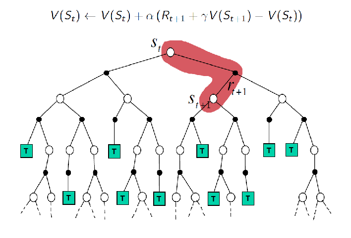
Visually, we can compare the three algorithms discussed so far:

MC Update	TD Update

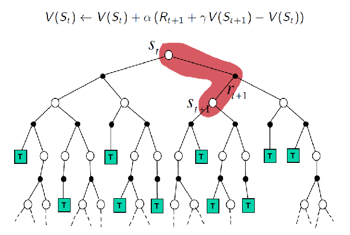And just to be complete, for DP method we know all transition probabilities, henc we can take into account all possibilities

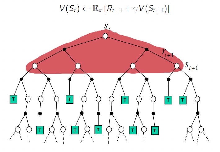
In this sense, TD(0) can be seen as taking samples over this DP backup, which also “bootstraps”

	Needs Model	Sampling	Bootstrapping
DP	Yes	No	Yes
MC	No	Yes	No
TD	No	Yes	Yes

Finally, algorithmically for TD(n):

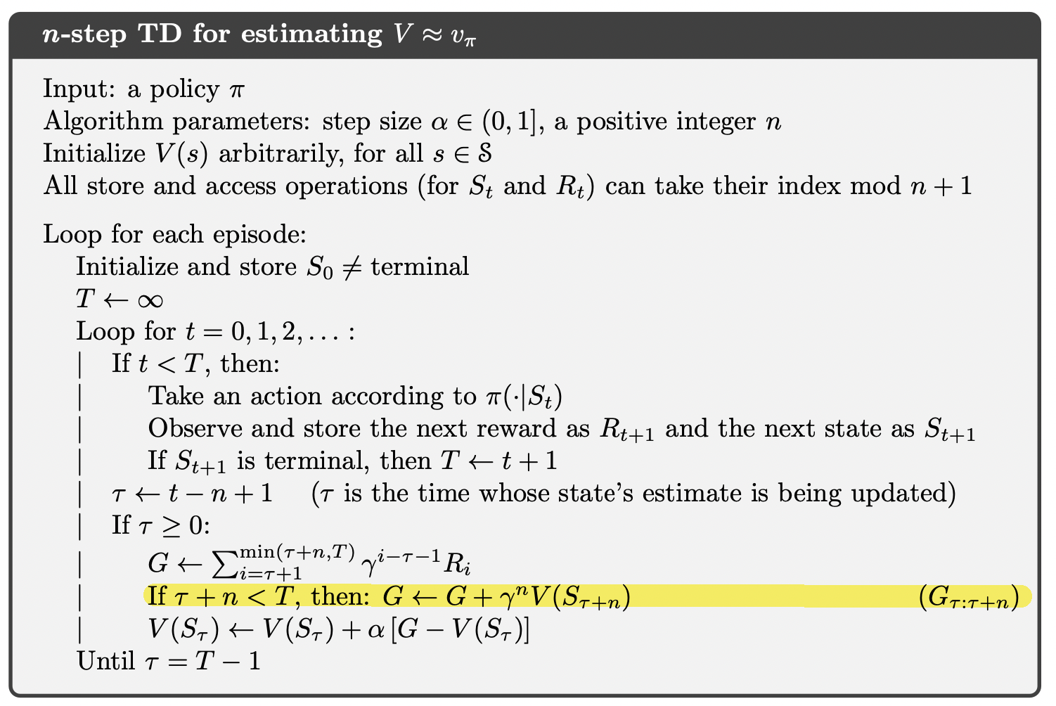
MC v.s. TD Methods

Here we compare some features of using MC v.s. TD to perform policy evaluation:

	MC	TD(0)
Learn before/without knowing final outcome	No	Yes
Target for update	$G_t$ which is a real return	estimate $R_{t+1} + \gamma v(S_{t+1})$ can be biased
Variance	High, because single branch + long episode means uncertainy builds up quickly	Low, because now depend on one random action, transition, and reward
Bias	no bias	not proven, has shown bias upperbound
Sentitive to Initial Value	no	yes, can affect convergence speed
Convergence Properties	Converges	Converges
Convergence Speed	Slow	Fast
used with Function Approximation	Little problem	often has problem converging
Storing Tabular Data	Yes	Yes

The still remaining concern but both still requires some kind of table to store value for each state, and/or action. For example, we update $Q$ estimate by storing the values of $(s,a)$ in a tabular representation: finite number of state-action pair.

However, as you can imagine many real world problems have enormous state and/or action space so that we cannot really tabulate all possible values. So we need to somehow generalize to those unknown state-actions.

Aim: even if we encounter state-action pairs not met before, we want to make good decisions by past experience.

Value Function Approximation: represent a (state-action/state) value function with a parametrized function instead of a table, so that even if we met an inexperienced state/state-action, we can get some values. (which will be discussed in the next section)

For Example: using TD for policy Evaluation

Consider the following MDP, with reward $0$ except for one state:

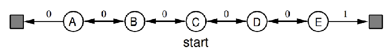
So that essentially there are:

two terminate states, so your optimal policy is to just move right.
And suppose my current policy $\pi$ is random left or right at equal probability, we want to evaluate this policy $\pi$ .

Let us use TD(0) learning and have initial values $V(S)=0.5$ for non-terminal states and $V(S_T)=0$ for those temrinal states.

we take $\alpha=0.1$, $\gamma=1$
then we update the estimate per time-step following TD(0) algorithm

With which we arrive at:

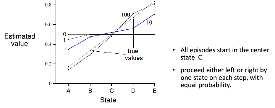
so after 100 episodes seen, we see it is going to converge to the true value.

Interestingly, from here we can ask: what is the episode encountered (see the line annotated by number 1) for the so that TD(0) only end up updated $V(A)\gets 0.45$?

realize that if you calculate anything from $V(S)\to S’ \neq S_T$ you will get no change in value, still $0.5$. For instance:
\[V_A \gets V_A + \gamma (R + V_B - V_A) = 0.5 + 1 \cdot (0) = 0.5\]
but things change only if you ended up at $V_T$ on the left, so that you get
\[V_A \gets V_A + \gamma (R + V_T - V_A) = 0.5 + 0.1 \cdot (0 + 0 -0.5) = 0.45\]

Therefore the episode just needs to hit left end state.

In this example, we can also compare the MC and TD variance

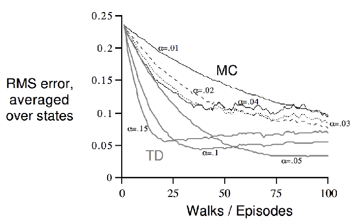
and note that MC achieves least MSE, while TD is performing MLE.

TD Control

In the end all people care is to get the optimal policy, rarely just to evaluate. Hence we need to use the evaluation/learning and do control

Intuitively: we can just apply TD to the $Q(S,A)$, and use $\epsilon$-greedy policy improvement as we have proven to work with MC methods

as long as we have some form of alternating policy evaluation and policy improvement, following Generalized Policy Iteration mos algorithms typically converge to the optimal policy

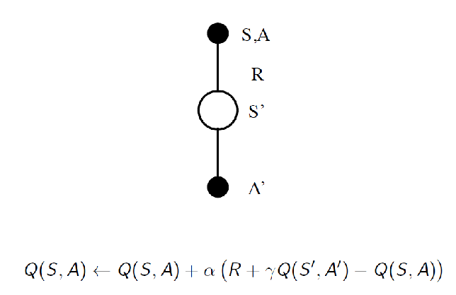
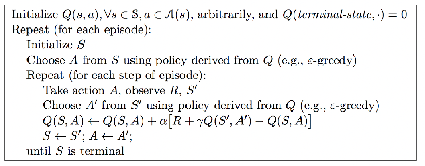
SARSA

SARSA: Essentially TD(0) learning for one step followed immediately by $\epsilon$-greedy policy improvement.

intuitively, it follows the Generalized Policy Iteration style

Sarsa converges with probability 1 to an optimal policy and action-value function, under the usual conditions on the step sizes $\sum \alpha^2 < \infty$, as long as all state–action pairs are visited an infinite number of times and the policy converges in the limit to the greedy policy (GLIE, which can be arranged, for example, with $\epsilon$-greedy policies by setting $\epsilon = 1/t$).

Given a single move/step $(S,A,R,S’,A’)$ we can perform an update using TD(0) equation:

Then, instead of waiting it to cnverge we can directly perform update, hence the algorithm becomes

where notice that essentially I improve my policy by picking better $A$ using $\epsilon$-greedy, and then ask my model to update accordingly.

this is on-policy control (i.e. behavior policy $\pi_b$ is the same as evaluation policy $\pi_e$)
on-policy as you already chosen your action while doing policy improvement
and recall that for convergence to the optimal greedy policy, you will need $\epsilon$ to decrease (i.e. the GLIE)

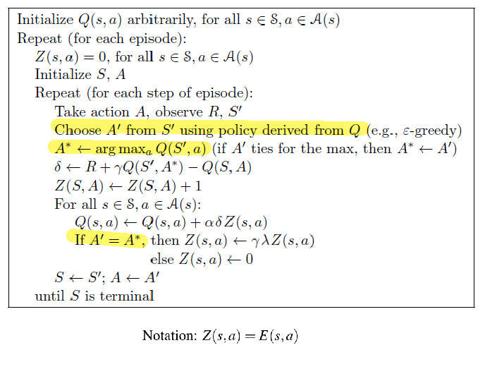
Q-Learning

Q-Learning: Most important and widely used today. It is motivated by having the learned action-value function, $Q$, from TD updates to directly approximates $Q_*$, the optimal action-value function, independent of the policy being followed.

dramatically simplifies the analysis of the algorithm and enabled early convergence proofs (is proven to converge)

All that is required for correct convergence is that all pairs continue to be updated. Under this assumption and a variant of the usual stochastic approximation conditions (i.e. $\sum \alpha^2 < \infty$) on the sequence of step-size parameters, $Q$ has been shown to converge with probability 1 to $Q_*$.

Now, the algorithm is that you are not choosing $A’$ from the current policy $\pi$, but update using greedy policy $\mathrm{greedy}(\pi)$

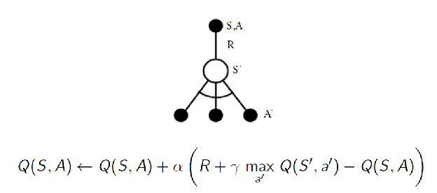
hence this is off-policy

your update is to estimate a greedy policy (i.e. optimal policy). This could have you, for example picking leftest action
but when I sample, I use $\epsilon$-greedy policy, meaning that I might have ended up in a differnt state. e.g. by picking the rightest action
but it is proven that it still converges to the optimal policy quickly

Algorithm:

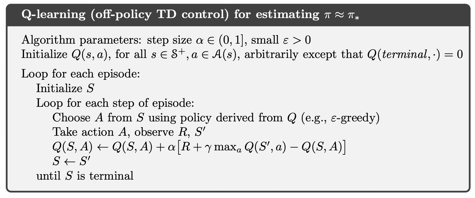
where here I improve my policy by picking better $A$ using $\epsilon$-greedy, but then ask my model to update the greedy policy.

This is widely used as there are early theoretical proofs to show it always converge to the optimal policy. But note that
but SARSA + greedy is still different than Q-Learning
so under the usual stochastic approxmation conditions with step size, and using GLIE, i.e. $\epsilon$ decreasing, both SARSA and Q-Learning will converge to the optimal value/policy. So what is the different between using them?

For Example: Cliff Walking

Consider the following cliff walking problem, where we want to use the SARSA and Q-learning to find the optimal policy given fixed $\epsilon=0.1$. Then eventually you will see the following performance

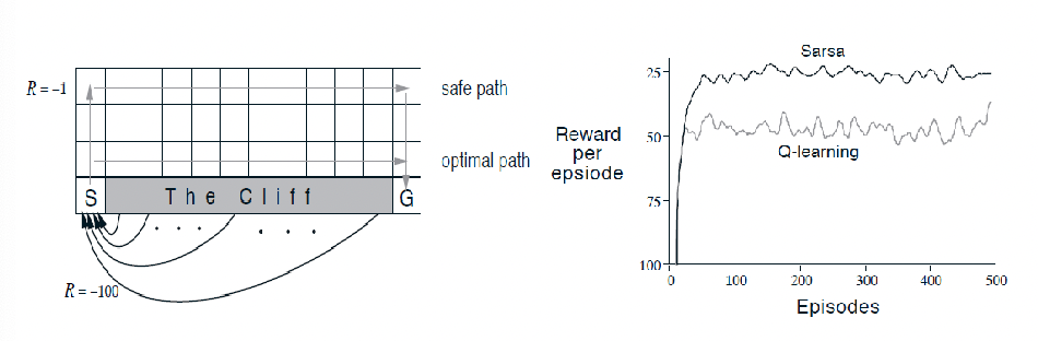
however, here we notice that Q-learning is doing worse. This does not contradict our previous conclusions because:

Q-learning aims to directly learn the optimal policy without taking into account the behavioral policy (i.e. $\epsilon=0.1$). Hence it learns the optimal path but occasionally falls off the cliff due to $\epsilon=0.1$
SARSA aims to learn the policy taking into account the behavioral policy and hence picks the safer path
but at the end of day, if we decrease $\epsilon \to 0$, then both converge to the same optimal path

But why would you want to have $\epsilon$-greedy policy used as behavioral policy when deployed?

in cases such as automonomous driving, simulation environment might be too optimistic and you may want your model to be more robust to random errors, as shown in the cliff case
so in that case SARSA could be prefered, which might not give you the optimal $Q$ values hence more robust

DP v.s. TD Methods

We can compare the backup diagrams and realize that our update forms corresponds a lot to DP=Bellman Equations while TD=sampling Bellman Equations

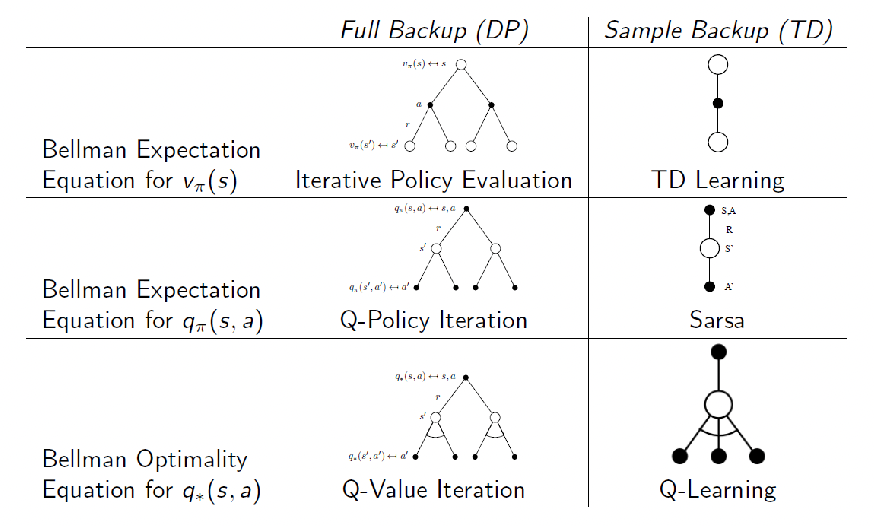
This becomes much clearer if we compare the update equation used:

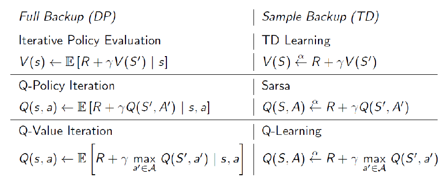
where $x \xleftarrow{\alpha} y$ means the update $x \gets x+ \alpha (y-x)$

so that Q-learning is sampling Bellman Optimality from DP
SARSA is like sampling from Bellman Expectation from DP

TD($\lambda$) and Eligibility Traces

We want to expand the basic TD(0) idea which can perform per step update (no wait for $G_t$) and MC which involves deep updates. Specifically, you will see how those relate to the idea of TD($\lambda$), and eventually see a unified view of RL algorithmic solutions.

At the end of this section, you should

understand what TD$(\lambda)$ and eligibility traces are
have a picture of how existing algorithms are came up/organized

Then we can go into implementations with Deep NN in the next section.

TD($\lambda$)

Recall that TD(0) considers the update of one-step look ahead

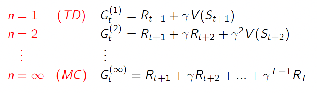
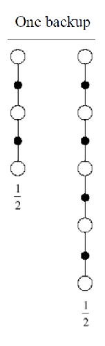
which basically aims to approximate the target $G_t = R_{t+1} + \gamma R_{t+2}+ \gamma ^2 R_{t+3}+ …= R_{t+1} + \gamma V(S_{t+1})$. We mentioned that we can easily extend this idea to $n$-step look ahead, which can be even generalized to the MC which gets to the terminate state:

\[\begin{align*} G_t^{(n)} &=R_{t+1} + \gamma R_{t+2}+ \gamma ^2 R_{t+3}+ ... \\ &= R_{t+1} + \gamma R_{t+2} + ... + \gamma^{n-1}R_{t+n} + \underbrace{\gamma^nV(S_{t+n})}_{\text{n-th step}} \end{align*}\]

Hence visually

Visual	TD(n) to MC Update Target

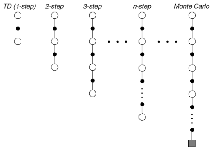Intuition: We can perhaps combine both MC and TD, and use all the information in the sample. So that instead of a single $n$-step return, we can average/combine all the $n$-step return.

For instance, consider you have a 2 and 4 step return computed, we can consider

Data We Have	Target
	$\frac{1}{2} G^2 + \frac{1}{2} G^4 = \frac{1}{2}\sum G^{(n)}$

So the question is what is a good way to combine those information?

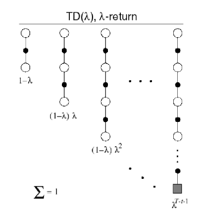
$\lambda$-Return: compute $G_t^\lambda$ which combines all $n$-step return $G_t^{n}$ using weight $(1-\lambda )\lambda^{n-1}$, which decays each future by $\lambda$ while summing up to $1$. This means that given all returns:
\[G_t^\lambda = (1-\lambda) \sum_{n=1}^\infty \lambda^{n-1} G_t^{(n)}, \quad G_t^{(n)} = R_{t+1} + \gamma R_{t+2} + ... + \gamma^{N}V(S_{t+N})\]
and hence your update equation becomes
\[V(S_t) \gets V(S_t) + \alpha (G_t^\lambda - V(S_t))\]
however, since this means you are adding both long episodes (MC) and short ones (TD), you will get

both high bias and big variance (from MC and TD)

you need a delay as it waits until terminal state (based on definitino $n=T$ here is the terminal state)

using bootstrapping because we calculate $G_t^{(n)}$ using TD method, hence sensitive to initialization

so even in TD(0) we can get rid of a lot of those problems. Meaning that TD($\lambda$) is not really used in practice. But this did provided the theoretical foundation for the eligibility trace, which is very useful.

Visually, the weights look like

Using All Information	Weights on Early $G_t^{(n)}$ decays = less important

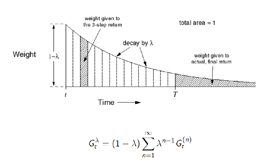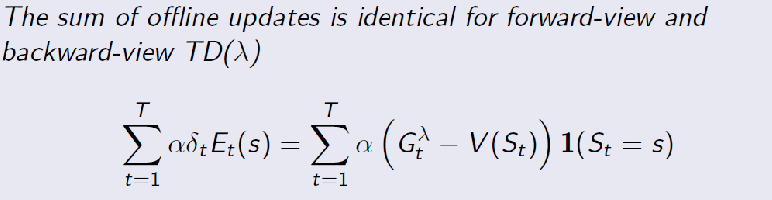
Note that in the forward-view, the weights need to sum up to $1$. This means in case if you have a finite horizon, as shown in the figure above you need to adjust your last weight so that your weights sum up to $1$.
\[G_t^{\lambda} = (1-\lambda) \sum_{n=1}^{T-t-1}\lambda^{n-1}G_{t}^{(n)}+\underbrace{\lambda ^{T-t-1}G_t}_{\text{last return}}\]

for instance, if you have three $G_t^{(n)}$, and $\lambda = 0.5$, then the weights will be $0.5, 0.5^2, 1-(0.5+0.5^2)$

So how do we improve this theoretical idea. Consider viewing TD($\lambda$) as a forward view as we are looking into the future

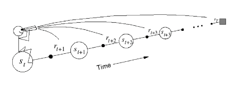
This forward view provides theory, the backward view provides mechanism/practicality

I would like to fix the following problems in this algorithm:

get a sample and can update like TD(0) per time step (instead of waiting)
combines information like TD($\lambda$) but hopefully avoid those bias and variance

Eligibility Trace

Heuristics: what are the useful features of the forward view TD($\lambda$) update?

frequency heuristics: most visited states should be more important (=need to have some kind of memory to know that it was visited in the past)

achieved by constantly adding the history and yet decaying like TD($\lambda$). i.e. add past eligibility but scaled: $\lambda E_{t-1}$

recent heuristic: most recent states should be also important

add a weight of $1$ (the indicator function)

So the idea technically comes form TD($\lambda$), which actually does

put more weight on the most recent state it has the highest weight
more weight on most visited states as they will be added more than once in the $\sum$

Eligibility Trace: essentially how do we design a weighting that achieves the above but also allow us to do per-step update?

Initialize the weight $E_0(s)=0$ for each state, and then consider
\[E_t(s) = \gamma \lambda E_{t-1}(s) + \mathbb{1}(S_t=s)\]
for $\mathbb{1}$ is the indicator function, and it records the “importance” for each state when the value function is updated (see later). But why this form? It turns out that this specific form allows for an (offline) equivalence of eligibility trace to TD($\lambda$) forward view.

For example, consider you are rolling out a single episode, and a state that is being visited 4 times in a row, not seen for a while, then seen twice, then seen once. Then, the eligibility trace of it looks like:

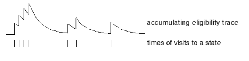
therefore, it satisfied what I needed:

if a state is visited more often, it gets a higher eligibility trace (like in the beginning)
if a state is visited more recently, it automatically have a weight of $+1$

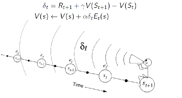
Backward View of TD($\lambda$): now we can use eligibility trace for value update.

Consider the TD error $\delta_t$ we used to update when doing TD(0):
\[\delta_t = \underbrace{R_{t+1} + \gamma V(S_{t+1})}_{\text{TD(0) target}} - V(S_t)\]
which enabled us to do per time-step update. Then, the idea is we weigh the per-time step error, such that if we accumulate the updates until the end of the episode, it will result in the same update as the forward TD($\lambda$). This is also called the offline equivalence (see next section), but with this constraint we end up with the weight called eligibility trace $E_t(s)$ which we showed before:
\[E_t(s) = \gamma \lambda E_{t-1}(s) + \mathbb{1}(S_t=s)\]
and hence the update rule:
\[V(s)\gets V(s) + \alpha E_t(s) \delta_t\]
so that this is given to each state, e.g. if we have 10 states, we get 10 eligibility traces. Intuitively, since $E_t(s)$ depended on history, it measures how much this state matters by looking in the past: to see if it is seen frequently, recently.

Visually, the backward view means we are using this loss $\delta_t$ using information in the past:

additionally

if $\lambda = 0$, then $E_t(s) =\mathbb{1}(S_t=s)$ and then eligibility trace becomes TD(0) update since we are then doing:
\[V(s)\gets V(s) + \alpha \delta_t(s)\cdot \mathbb{1}(S_t=s)\]
meaning we only update the ones we just saw

So this backward update now has the advantage of

including in the idea of forward TD($\lambda$) to use all the information we have
this is implementable as we don’t need to look n-step beyond (but behind). Meaning we can perform update per time step

Finally, we can show the algorithm of using Eligibility trace:

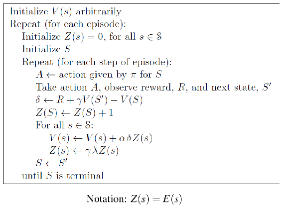
where basically the error is TD(0) error, but we are updating all states using eligibility trace per time step

this means we need to have two tables, one for eligibility per state and anther store the value per state
since now it is online (update per step), this backward is not equivalent to the forward view. But if we pick a step size sufficiently small, it is almost equivalent
practically, this online TD($\lambda$) updates is what we use and works

Note that

we are updating all states per time step, so even if you have just seen a state $S_t=B$, and $S={A,B}$, you still need to update both $S=A,S=B$ in the loop when updating $V(s)$. A hint is to notice that $\delta$ is not a function of state in the above algorithm.

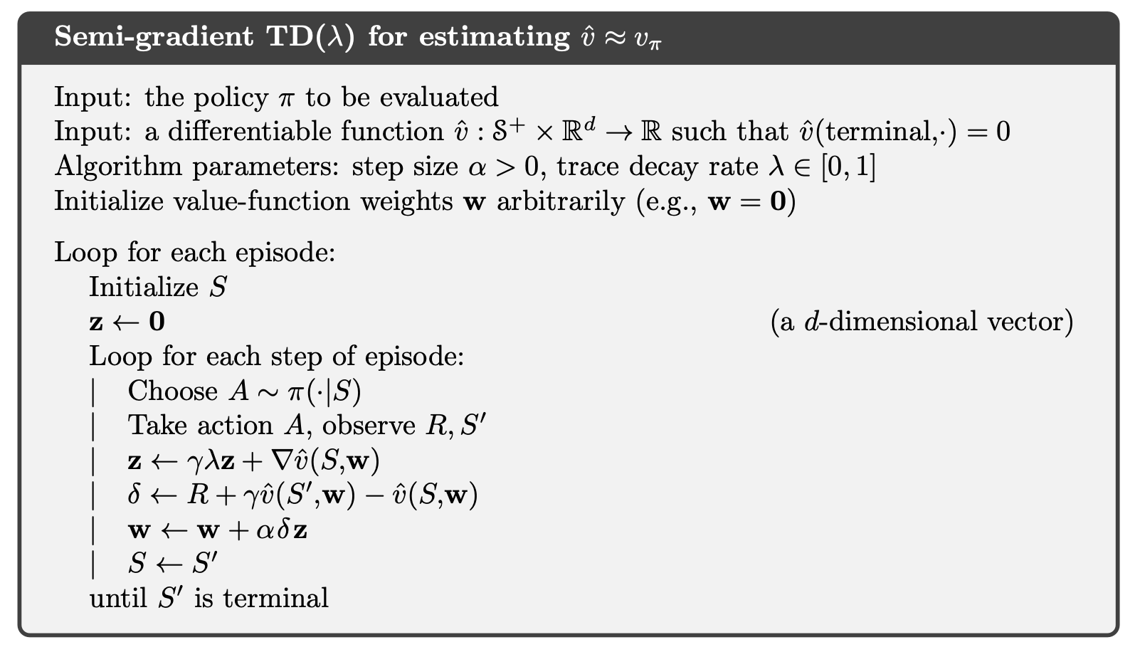
when used with value function approximation, the eligibility trace generalizes to
\[E_t(s) = \gamma \lambda E_{t-1}(s) + \nabla \hat{V}(S,w)\]
and algorithm looks like

Offline Equivalent of Forward and Backward Views

Finally, here we answer the question why did people decide to use specifically the weight in the form of $E_t(s)$

\[E_t(s) = \gamma \lambda E_{t-1}(s) + \mathbb{1}(S_t=s)\]

Offline Equivalence

Consider having your eligibility trace being updated/accumulated all the time, but you only update $V$ at the end. Recall that for the forward view, we also only update at the end. Now, you realize that

so if we were offline only learning the eligibility traces, your final updated $V$ will be the same as the forward view

so in offline mode you are essentially summing up all the errors of each state over all time but without updating $V$

so then the proof is to show that the this accumulated error is the same in forward view! But this proof is long so skipped

TD($\lambda$) Control

In the previous section we are essentially learning the value function, now we care about using it to find the optimal policy. The basic idea is again simple: we can apply this learning style to learn an optimal $Q_*(s,a)$.

Recall that to derive the backward eligibility trace we need to

derive the forward algorithm by considering the $n$ step look-ahead version of the TD error
use the eligibility trace in backward algorithm
show their offline equivalence

SARSA($\lambda$)

First, we consider the forward TD($\lambda$). Consider the $n$-step look ahead for SARSA's target

So that the $n$-step look ahead return is

\[q_t^{n} = R_{t+1} + \gamma R_{t+2} + ... + \gamma^{T-1} R_{t+n} + \gamma^n Q(S_{t+n})\]

Hence the forward view considers weighting those returns:

\[q_t^{\lambda} = (1-\lambda) \sum_{n=1}^\infty \lambda^{n-1} q_t^{(n)}\]

So the forward view of SARSA becomes:

\[Q(S_t, A_t) \gets Q(S_t,A_t) + \alpha (\underbrace{q_t^{\lambda}}_{\text{TD($\lambda$) target}} - Q(S_t,A_t))\]

and notice that using $\lambda=0$ we get back SARSA (which uses TD(0) target)

Then from it, we can find the backward view by building this eligibility trace knowing that

\[\delta_t = R_{t+1} + \gamma Q(S_{t+1}, A_{t+1}) - Q(S_t, A_t)\]

so then intuitively we can say that the eligibility trace is, with $E_0(s,a)=0$:

\[E_t(s,a) = \gamma \lambda E_{t-1}(s,a) + \mathbb{1}(S_t=s, A_t=a)\]

so that our update rule is:

\[Q(s,a) \gets Q(s,a) + \alpha E_t(s,a) \delta_t\]

essentialy:

target is stil SARSA target, but error is weighted by eligibility trace
so again two tables, one for Q and one for eligibility trace
and we skip the proof that this gives the same result as the forward view of SARSA if offline

Therefore, we get this SARSA($\lambda$) algorithm

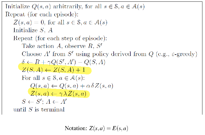
We can visualize the differences:

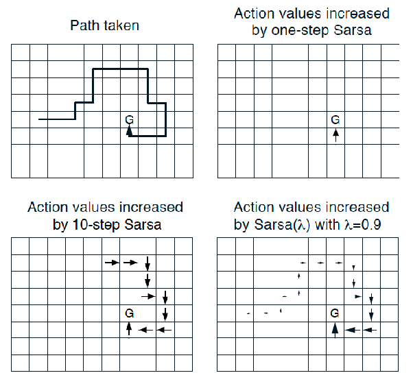
so that

if SARSA, then we only updated using only one “previous” step
if using 10-step SARSA, my last step will take into account my previous 10 steps equally
if using SARSA($\lambda$) with $\lambda=0.9$, then we update using all history weighted by eligibilty trace

Q($\lambda$)-Learning

There are many ways to do this, but you need to have some proof that it works. So here we use Watkins’s version. First recall that

Q-learning aims to do Bellman optimality directly each step
it is off-policy, and like SARSA, the update is per step (no need to wait)
both Q-learning and SARSA is proven to give you the optimal policy (under mild conditions)

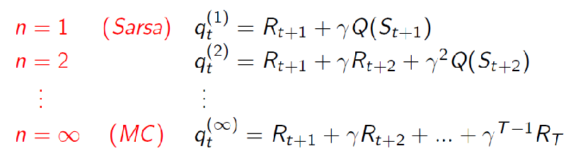
Now, consider Q($\lambda$). We first consider $n$-step look ahead of the target (different from SARSA’s target)

\[\begin{cases} \text{1-step}, & R_{t+1} + \gamma \max_a Q(S_{t+1}, a) \\ \vdots \\ \text{$n$-step}, & R_{t+1} + \gamma R_{t+2} + ... + \gamma^{T-1} R_{t+n} + \gamma^n \max_a Q(S_{t+n}, a) \end{cases}\]

But then, you have a problem that since Q-learning is off-policy, what does the forward view look like? In Watkin’s $Q(\lambda)$, we considers two terminate cases:

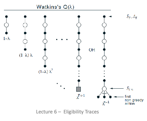
so that your last look-ahead either is

the actual terminate state
your behavior policy picked an action that is non-greedy

So that your backward view becomes

\[\delta_{t} = R_{t+1} + \gamma \max_a Q(S_{t+1}, a) - Q(S_t, A_t)\]

with eligibility trace

\[E_t(s,a) = \begin{cases} 1 + \gamma \lambda E_{t-1}(s,a) & \text{if }s=s_t, \text{ and } a\sim \epsilon\text{-greedy}(Q(s,a)) = \arg\max_{a} Q(s,a) \\ 0, & \text{if }a \neq \arg\max_{a} Q(s,a)\\ \gamma \lambda E_{t-1}(s,a) & \text{otherwise, i.e. not at } s_t \end{cases}\]

with the upadte rule being

\[Q(s,a) \gets Q(s,a) + \alpha E_t(s,a) \delta_t\]

Hence the algorithm looks like

so basically

if action I took w.r.t. to my current $\epsilon\text{-greedy}(Q)$ is the greedy action, then we do the normal eligibility trace update
if not, then reset all to zero, because we reached a “dummy terminal state” which we defined by next move being not greedy action (by this definition, we can still have equivalence of backward and forward view)
so again, my error is the Belmman Optimality Error using the $A^{*}$ from the greedy policy, but my behavior policy is to do $A’$ which is $\epsilon$-greedy. Hence this is off-policy as is Q-learning.

Recall that all algorithms we see here needs a tabular value. Hence for large state space/state-action space, those algorithms are slow due to this loop for all state/state-action.

This problem is solved by using function approximation: the only parameters are the parmeters of the functions which can spit out those values, which we will see in the next section.

Unified View of RL Solutions

All the basics of RL algorithms can be put in one picture, and we can understand their differences/similarities

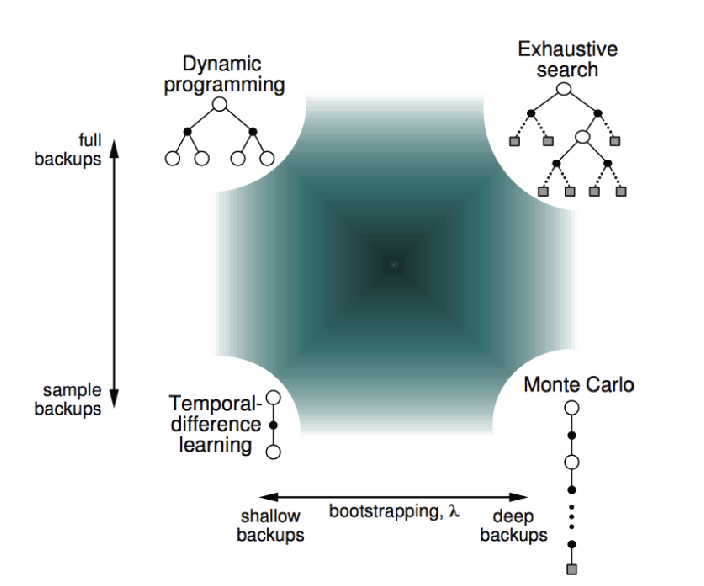
where

shallow means update only looks at 1 step, and deep is like MC (depth). This depth can be changed depending on n-step return and hence the $\lambda$ parameter weighting how many future you want to use.
full backup means you look at all possible neighbors (width)
in practice, all algorithms such as Q-learning and SARSA are based on sample backups, as the updates are faster and more efficient
MCTS with truncation and approximations would be similar to the exhaustive search on top right