ELEN6885 Reinforcement Learning part2
RL packages
Now we start to discuss using DL for modeling. Some commonly used packages include
Mainly for this course
- openAI
gymmainly an online environment for bench-marking for algorithm performance
Other
stable-baselines3implementations of many modern RL algorithmsrllibincludes ray tuning
Resources
- colab tutorial: https://colab.research.google.com/github/araffin/rl-tutorial-jnrr19/blob/sb3/1_getting_started.ipynb
- openai doc: https://www.gymlibrary.dev/
- stable-baselines3 doc: https://stable-baselines3.readthedocs.io/en/master/
OpenAI Gym
- Separate the implementation of the environment from the implementation of the learning algorithm.
- Make it easy to compare various RL algorithms on the same/standardized environment.
-
installation, e.g.
gym[mujoco] -
has many environments which can be treated as benchmark “datasets”
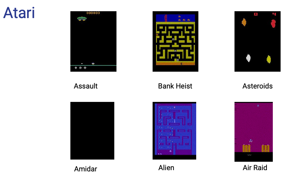
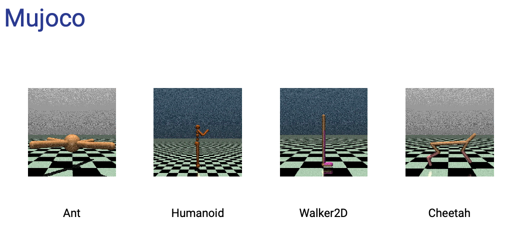
Control Atari Mujoco 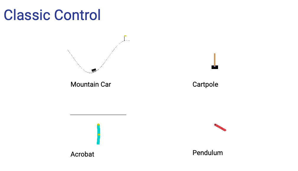
and many more
As basically they are interactive environments, the environment is what is implemented, meaning your job is to determine what action to take (i.e. your model) given your state (e.g. history of rgb pixels of the game), and environment gives you a reward and next state
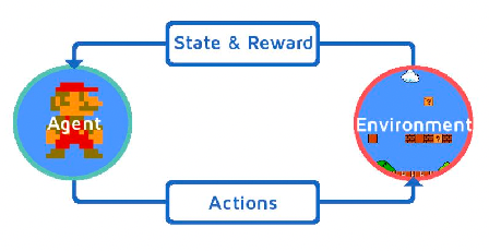
Specifically the environment will give you
- observation: the new state simulated by the environment
- reward: defined and computed by the environment
- done: A boolean indicating if episode has finished
- info: additional info used only for debugging
And the most important is the observation & action space for each environment:
- it will have an
action_spacespecifying what are the legal actionsDiscrete: A discrete space where $a(s) \in {0,1,…,n}$Box: An n dimensional continuous space with optional boundsDict: A dictionary of space instances such asDict({"position": Discrete(2), "velocity": Discrete(3)})
- it will have an
observation_spacespecifying what will be returned- e.g. RGB pixel values of the screen
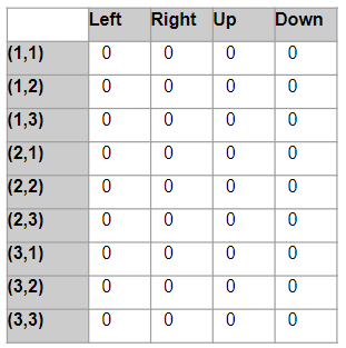
Examples: Cliff Walking Environment
The board is a 4x12 matrix, with (using NumPy matrix indexing):
[3, 0]as the start at bottom-left[3, 11]as the goal at bottom-right[3, 1..10]as the cliff at bottom-center
If the agent steps on the cliff, it returns to the start. An episode terminates when the agent reaches the goal.
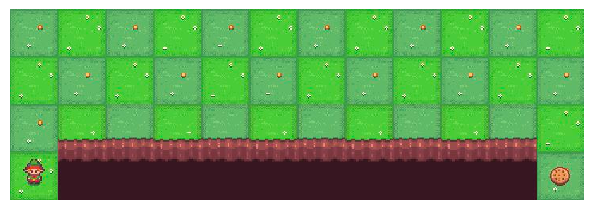
Reward
- Each time step incurs -1 reward, and stepping into the cliff incurs -100 reward.
Action Space: There are 4 discrete deterministic actions:
- 0: move up
- 1: move right
- 2: move down
- 3: move left
Observation Space: returned as a flattened index to represent the coordinate of the system
- There are 3x12 + 1 possible states. In fact, the agent cannot be at the cliff, nor at the goal (as this results in the end of the episode). It remains all the positions of the first 3 rows plus the bottom-left cell.
- The observation is simply the current position encoded as flattened index. You can easily convert back to coordinate system with
np.unravel_index
Example: Mujoco Humanoid
The 3D bipedal robot is designed to simulate a human. It has a torso (abdomen) with a pair of legs and arms. The legs each consist of two links, and so the arms (representing the knees and elbows respectively). The goal of the environment is to walk forward as fast as possible without falling over.
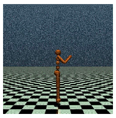
Action space is a Box(-1, 1, (17,), float32). An action represents the torques applied at the hinge joints.
-
action is a box has 17 different joints, each controlling torque from
[-1.0,1.0] -
example joints you can control:
hip_1 (front_left_leg), angle_1 (front_left_leg), hip_2 (front_right_leg), right_hip_x (right_thigh), right_hip_z (right_thigh), ...
Observation Space
- Observations consist of positional values of different body parts of the Humanoid, followed by the velocities of those individual parts (their derivatives) with all the positions ordered before all the velocities
Rewards: the reward consists of four parts:
-
healthy_reward: Every timestep that the humanoid is alive -
forward_reward: A reward of walking forward -
ctrl_cost: A negative reward for penalizing the humanoid if it has too large of a control force. -
contact_cost: A negative reward for penalizing the humanoid if the external contact force is
Using OpenAI Gym
A minimal working example would be:
import gym
env = gym.make("CartPole-v1")
state = env.reset()
for _ in range(1000):
    env.render()  # show a window on your screen. In colab notebook more needs to be done
    action = env.action_space.sample()  # random policy
    state, reward, done, info = env.step(action)
    if done:
        state = env.reset()
env.close()
Stable-Baselines-3
Stable Baselines3 (SB3) is a set of reliable implementations of reinforcement learning algorithms in PyTorch.
Where OpenAI gym focuses on the environment, stable-baselines-3 focuses on the learning. But of course it is easily integratable with OpenAI gym. Smoe additional features include
- access to most popular deep reinforcement learning algorithms. Ex: DQN, PPO, A2C, DDPG
- allow you to implement deep reinforcement learning solutions in just a few lines
- vectorized training in parallel (e.g. instantiate parallel copies of agents)
import gym
from stable_baselines3 import PPO

env = gym.make("CartPole-v1")  # use mode='rgb_array' to return game image as state

# training
model = PPO("MlpPolicy", env, verbose=1) # multilayer perceptron + feedin environment
model.learn(total_timesteps=10_000)

# testing
obs = env.reset()
for i in range(1000):
    action, _states = model.predict(obs, deterministic=True)
    obs, reward, done, info = env.step(action)
    env.render()
    if done:
        obs = env.reset()
env.close()
Function Approximation
Recall that all evaluation and control algorithms we discussed are tabular methods (e.g. $Q(s,a)$)
- Each update will only change the value of one state or one state-action pair, i.e., an entry in the lookup table
- The lookup table may become unmanageable when the number of “states” or “state-action” pairs goes up. For instance, what if we have a continuous action space?
- also needed a way to keep exploring, because we needed to estimate values of a lot of states to be accurate
Use function approximation to treat $V(s)$ or $Q(s,a)$ as functions, i.e. we consider instead of tables, parameters of a function such that:
- for $V$: $S\to \mathbb{R}$
- for $Q: S,A \to \mathbb{R}$
so we consider $V(s,w)$ and $Q(s,a,w)$ for $w$ being the weights/parameters of the function
Function approximation methods has advantages for cases such as
- evaluate/predict $v(s)$ and $q(s, a)$ for large or high-dimension state space
- evaluate/predict $v(s)$ and $q(s, a)$ for continuing tasks (non-episodic)
- evaluate/predict $v(s)$ and $q(s, a)$ for partially observable problems
- because we can extrapolate from the experienced samples (e.g. states)
and is usally trained with supervised training
- e.g. given a $(s,G_t(s))$ pair, ask the model to do learn it
- use SGD to minimize the objective function such as MSE between $\hat{V}(s,w)$ and $V(s)$
Value Function Approximation
We would like to consider $\hat{V}(s,w)$ and $\hat{Q}(s,a,w)$ parameterized by $w$:
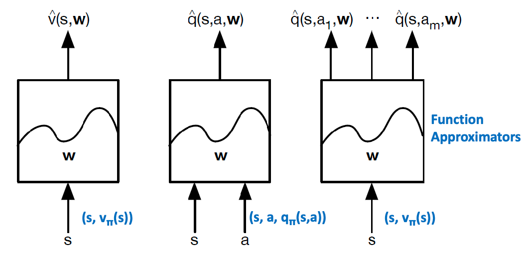
where the target $V_\pi(s)$ and $Q_\pi(s,a)$ are basically predefined by the specific algorithms we want to use and our model aims to model them.
- In general we can have three types of modelling, where the last one modelling $Q$ from $V$ is not used often in practice
- for MC methods, bascially $V_\pi(s) = G_t$ is used as target, and it differs if you do TD(0), for instance
- since those are aimed to improve on tabular methods, dimensoinaltiy of $w$ is typically much smaller of states $\vert S\vert$, and highly related to how many features you want to encode in each state
- finally, notice that updating one weight will influence value for all states (cf. tabular methods)
There are many ways to construct your function approximator, e.g.:
-
Linear: consider we having three features of a state $s=[s_1,s_2, s_3]^T$. Then we can do:
\[V(s,w) = s_1 w_w + s_2 w_2 + s_3 w_3 = [s_1, s_2,s_3]^T \begin{bmatrix}w_1\\ w_2\\ w_3\end{bmatrix}\]or you can construct nonlinear features usch as $w_1*w_2$
-
non-linear: using neural networks
- decision tree
- etc.
Here we consider differentiable function approximation methods.
For instance, let $w$ be a column vector. Then we can consider
\[J(w) = \mathbb{E}[ (\hat{V}(s,w) - V_\pi(s) )^2 ]\]to minimize this loss using SGD (single sample per batch) type approach to consider
\[\Delta w = - \frac{1}{2} \alpha \nabla_w J(w)\]if you perform the chain rule and take derivatives you get:
\[\Delta w = \alpha \mathbb{E}_\pi [(v_\pi(s) - \hat{v}(s,w)) \nabla_w \hat{v}(s,w)]\]Finally, as we are doing SGD:
\[\Delta w = \alpha \underbrace{(v_\pi(s) - \hat{v}(s,w))}_{\text{prediction error}} \underbrace{\nabla_w \hat{v}(s,w)}_{\text{gradient}}\]note that
- the above form is generic if you use MSE
- $v_\pi(s)$ depends on what algorithm you use, e.g. MC means $v_\pi(s) = G_t$ is calculated at the end of episode.
Example: Simple SGD updates
Let the target be $y$, and the input features are 1-D $x$. So that you get the following dataset
\[(x_1, y_1), (x_2, y_2), \dots, (x_n, y_n)\]Suppose your approximator has two parameters:
\[\hat{V}(x) = w_1 + w_{2} x\]Then your MSE loss is simply:
\[J(w) = \sum\limits_{i=1}^{n} (\hat{V}(x_i) - y_i)^2 = \sum\limits_{i=1}^{n} (w_1 + w_2 x_i - y_i)^2\]Therefore, in the case of SGD your per step weight update with learning rate $\eta$ is
\[\begin{bmatrix} w_1\\ w_2 \end{bmatrix} \gets \begin{bmatrix} w_1\\ w_2 \end{bmatrix} - \eta \nabla_w J(w) = \begin{bmatrix} w_1\\ w_2 \end{bmatrix} - \eta \begin{bmatrix} 2(w_1 + w_2 x_i - y_i)\\ 2x_i(w_1 + w_2 x_i - y_i) \end{bmatrix}\]RL Prediction with Value Approximation
Now, we employ VFA methods to perform RL. Recall that in general we need two things:
- evaluation/prediction of $v_\pi(s)$ and $q_\pi(s,a)$
- control/planning to find optimal policy (usually by using $q_\pi(s,a)$)
Here, we first discuss the problem of prediction. As essentially it becomes supervised learning
- agent interact using policy $\pi$ to collect experience/dataset
- since the collected signals are only rewards, you usually need to then specify a target for the model to learn
- now you have a supervised dataset, and you can use SGD to train your model
For instance:
-
if you are using MC methos, then your computed target is simply $G_t = \sum\limits_{k=t}^{T} \gamma^{k-t} r_k$ so that your weight updates become
\[\nabla w = \alpha \underbrace{( \textcolor{red}{G_t} - \hat{v}(S_t,w) )}_{\text{prediction error}} \nabla_w \hat{v}(S_t,w)\] -
if you are using TD methods, then technically your target is $R_{t+1}+\gamma V_\pi(S_{t+1})$, but since you don’t know $V_\pi$, you consider:
\[\nabla w = \alpha \underbrace{( \textcolor{red}{R_{t+1}+\gamma \hat{v}(S_{t+1},w)} - \hat{v}(S_t,w) )}_{\text{prediction error}} \nabla_w \hat{v}(S_t,w)\]note that as our target is technically also parametrized by $w$ but we did not take its gradient, it is also called semi-stochastic gradient descent. (e.g. in DQN, we would use old $\hat{v}(S_{t+1},w^-)$ as targets and update it over time)
-
for TD($\lambda$), the target is $G_t^\lambda$:
\[\nabla w = \alpha \underbrace{( \textcolor{red}{G^{\lambda}_t} - \hat{v}(S_t,w) )}_{\text{prediction error}} \nabla_w \hat{v}(S_t,w)\]which is the forward-view. The backward-view update is shown in the section TD($\lambda$) with Value Function Approximation
Linear Function Approximation
We can consider a simple case study of using linear function approximation to predict $v_\pi(s)$.
Your general pipeline would be:
- determine your feature representation $x(s)$ for each state $s \in S$:
-
define your model. Here we consider a linear approximator, we consider:
\[\hat{v}(S, w) = \boldsymbol{x}(S)^{T} \boldsymbol{w} = \sum\limits_{j=1}^{n} x_{j} (S)w_j\] -
define your objective: consider given the true value $v_\pi(S)$:
\[J(\boldsymbol{w}) = \mathbb{E}_\pi[(v_\pi(S) - \boldsymbol{x}(S)^{T} \boldsymbol{w} )^2]\] -
perform gradient descent. Using SGD the update rule for weights become:
\[\begin{align*} \nabla_{w} \hat{v}(S, w) &= \boldsymbol{x}(S)\\ \Delta w &= \alpha \underbrace{(v_\pi(S) - \boldsymbol{x}(S)^{T} \boldsymbol{w} )}_{\text{prediction error}} \boldsymbol{x}(S)\\ \end{align*}\]
Note that in practice:
- very important to choose the right features and the representations
- for linear approximators, the gradient $\nabla_{w} \hat{v}(S, w) = \boldsymbol{x}(S)$ is just the feature vectors
Special Example: modelling table look up
We can actually use a linear approximator and get back tabular methods.
- we can make feature to be onehot of states
- then weights are basically the values in the table lookup
Then a linear approximator gives
\[\hat{v}(S, w) = \boldsymbol{x}(S) = \begin{bmatrix} 1(S=s_1)\\ \vdots\\ 1(S=s_n) \end{bmatrix} \cdot \begin{bmatrix} w_1\\ \vdots\\ w_n \end{bmatrix}\]so that essentially $\hat{v}(S_i) = w_i$ is like a table lookup.
MC with Value Function Approximation
Recall that for MC methods, we consider a target of $G_t$. Therefore:
-
experiences $(S_i, A_i, R_i)$ and compute $(S_i, G_i)$ pairs to get training data
\[(S_1, G_1), (S_2, G_2), \dots, (S_T, G_T)\] -
then just perform supervised learning to train your model
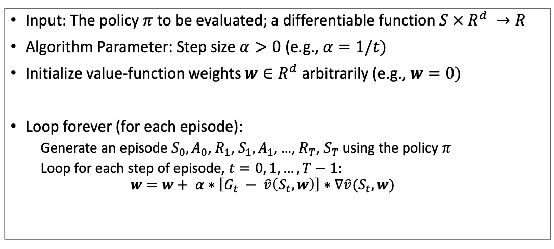
Note that
- theoretically, in order to guarantee convergence, $\alpha$ should be decreasing but needs infinite visit of all states (the usual stochastic assumption) $\sum \alpha = \infty, \sum \alpha^2 < \infty$, for instance $\alpha = \frac{1}{t}$
- but in reality people just use constant $\alpha$ and it works fine
TD(0) with Value Function Approximation
Recall that the TD Target $R_{t+1} + \gamma \hat{v}(S_{t+1},w)$ is biased as we are using $\hat{v}(S_{t+1},w)$ to estimate $v\pi(S_{t+1})$.
But you can still regardless compute the supervised signal as $(S_i, R_{i+1} + \gamma \hat{v}(S_{i+1},w))$ hence
-
collect experience hence a dataset of
\[(S_1, R_2 + \gamma \hat{v}(S_2,w)), (S_2, R_3 + \gamma \hat{v}(S_3,w)), \dots, (S_{T-1}, R_T + \gamma \hat{v}(S_T,w))\] -
then again supervised training on your $\hat{v}(S,w)$ with SGD:
\[\nabla \boldsymbol{w} = \alpha \underbrace{(R_{t+1} + \gamma \hat{v}(S_{t+1},w) - \hat{v}(S_t,w))}_{\text{prediction error}} \nabla \hat{v}(S_t,w)\]or sometimes people just write (as TD is used often)
\[\nabla \boldsymbol{w} = \alpha \delta \nabla \hat{v}(S_t,w)\]
Then the rest of the algorithm is basically the same as the MC version. Note that
- again, this is not fully stochastic = semi-stochastic gradient as that target $R_{i+1} + \gamma \hat{v}(S_{i+1},w)$ is parameterized yet no gradient is taken
- examples of this type of algorithm is DQN, and active research is on improving this semi-gradient algorithm
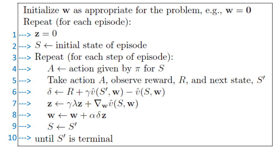
TD($\lambda$) with Value Function Approximation
The target for TD($\lambda$) is $G_t^\lambda$, which is a weighted sum of TD targets and is still biased of the true value $v_\pi(S_t)$.
But regardless:
-
collect experience hence a dataset of
\[(S_1, G_1^\lambda), (S_2, G_2^\lambda), \dots, (S_T, G_T^\lambda)\] -
then again supervised training on your $\hat{v}(S,w)$ with SGD. First the forward view is simply:
\[\nabla \boldsymbol{w} = \alpha \underbrace{(G_t^\lambda - \hat{v}(S_t,w))}_{\text{prediction error}} \nabla \hat{v}(S_t,w)\] -
then we derive the update rule being the backward view:
\[\begin{align*} \delta_{t} &= R_{t+1} + \gamma \hat{v}(S_{t+1},w) - \hat{v}(S_t,w)\\ E_{t} &= \gamma \lambda E_{t+1} + \nabla \hat{v}(S_t,w) \\ \nabla \boldsymbol{w} &= \alpha \delta_{t} E_{t} \end{align*}\]
So we get the algorithm being:
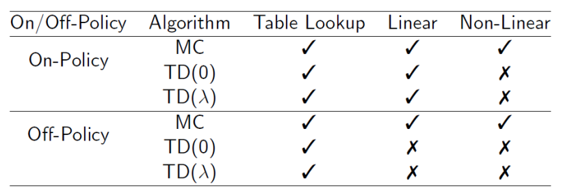
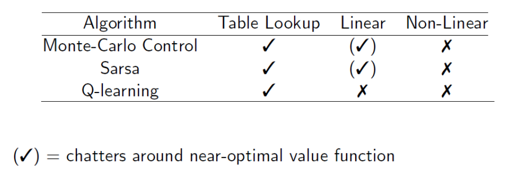
Convergence of Prediction Algorithms
In general TD methods are fast to learn but are unstable.
RL Control with Function Approximation
How do we find the optimal policy once we estimated the value or action-value function using VFA?
Recall that as we are in the case of model-free control, we generally consider:
- estimate action-value function $Q_\pi(S,A)$
- policy improvement using $\epsilon$-greedy policy of $Q_\pi(S,A)$
Hence the general policy iteration (still applies) basically looks like
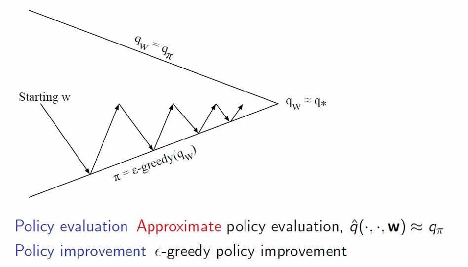
As policy improvement is based on $Q_\pi(S,A)$, all we need to do is to estimate $Q_\pi(S,A)$ using VFA. This essentially is the same as fitting $V_\pi(S)$ but use $Q$ instead in formulas.
Hence our model considers
\[\hat{q}(S,A,w) \approx \hat{q}_\pi(S,A)\]then to fit it, we consider
\[J(\boldsymbol{w}) = \mathbb{E}_{\pi}[(\hat{q}(S,A,w) - q_\pi(S,A))^2]\]and using SGD the gradient is
\[\nabla w = \alpha \underbrace{(q_\pi(S,A) - \hat{q}(S,A,w))}_{\text{prediction error}} \nabla \hat{q}(S,A,w)\]and based on different algorithms you use different targets to compute $q_\pi(S,A)$
As it is basically the same as the value function case, we will quickly show:
-
for MC methods, the target is $G_t$
\[\nabla w = \alpha \underbrace{(\textcolor{red}{G_t} - \hat{q}(S_t,A_t,w))}_{\text{prediction error}} \nabla \hat{q}(S_t,A_t,w)\] -
for TD(0), the target is the estimated TD target $R_{t+1} + \gamma \hat{q}(S_{t+1},A_{t+1},w)$
\[\nabla w = \alpha \underbrace{(\textcolor{red}{R_{t+1} + \gamma \hat{q}(S_{t+1},A_{t+1},w)} - \hat{q}(S_t,A_t,w))}_{\text{prediction error}} \nabla \hat{q}(S_t,A_t,w)\] -
for forward-view TD($\lambda$) the target is $G_t^\lambda$
\[\nabla w = \alpha \underbrace{(\textcolor{red}{G_t^\lambda} - \hat{q}(S_t,A_t,w))}_{\text{prediction error}} \nabla \hat{q}(S_t,A_t,w)\]and the backward view update rule is
\[\begin{align*} \delta_{t} &= R_{t+1} + \gamma \hat{q}(S_{t+1},A_{t+1},w) - \hat{q}(S_t,A_t,w)\\ E_{t} &= \gamma \lambda E_{t+1} + \nabla \hat{q}(S_t,A_t,w) \\ \nabla \boldsymbol{w} &= \alpha \delta_{t} E_{t} \end{align*}\]
the algorithms are again basically the same as the value function case.
Convergence of Control Algorithms
Problem mostly occurs when you do TD and Non-linear function approximation.
Batch Method for RL Applications
Before, we are talking about SGD which uses a sample and throw it away after updates.
Aim: We can be more sample efficient by sampling a batch and perform updates. Additionally, it also provides a better estimate to solve the least square problem.
Consider a given experience dataset $D$ consisting of state-value pairs provided:
\[\mathcal{D} = \{ (s_1, v_1^{\pi}), (s_2, v_2^{\pi}), ..., (s_T, v_T^{\pi}) \}\]then the best parameter that best fits $v_\pi$ obviously needs to perform least square on all of them
\[LS(\boldsymbol{w}) = \sum_{t=1}^T (v_t^{\pi} - \hat{v}(s_t,w))^2 = T \cdot \mathbb{E}_{\pi}[(v^{\pi} - \hat{v}(s,w))^2]\]or $T$ times the average error you make. Naive SGD for each sample would not work as recall
- each piece of experience would be correlate as they will come from real experience
- but fitting VFA assumes that the samples are independent
therefore, they will be techniques such as experience replay to shuffle the order so data appears IID:
-
given an experience consisting of state value pairs
\[\mathcal{D} = \{ (s_1, v_1^{\pi}), (s_2, v_2^{\pi}), ..., (s_T, v_T^{\pi}) \}\] - repeat
-
sample state, value for experience
\[(s_t, v_t^{\pi}) \sim \mathcal{D}\] -
update the parameters using SGD
\[\Delta w = \alpha (v_t^{\pi} - \hat{v}(s_t,w)) \nabla \hat{v}(s_t,w)\]
-
-
converges to LS solution:
\[\boldsymbol{w} = \arg\min_{w} LS(\boldsymbol{w})\]
This basically is the SGD version of experience replay in DQN.
Brief Introduction of DQN:
Here we will deal with non-linear function approximation and the problem of correlation.
Non-linear neural networks: needs a static training set + uncorrelated IID data during training
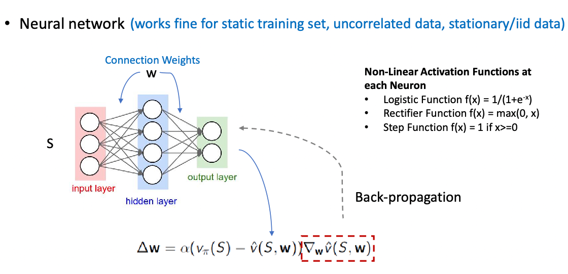
DQN uses experience replay to remove correlations between consecutive samples of data and fixed Q-target to stabilize the learning process.
The overall algorithm consists of:
- take action $a_t$ in state $s_t$ and observe reward $r_t$ and next state $s_{t+1}$
- store transition $(s_t, a_t, r_t, s_{t+1})$ in replay memory $D$
- sample random minibatch of transitions $(s_j, a_j, r_j, s_{j+1})$ from $D$
-
compute Q-learning targets w.r.t to old network $\boldsymbol{w}^-$ and optimize MSE:
\[L(\boldsymbol{w}) = \mathbb{E}_{(s_j, a_j, r_j, s_{j+1}) \sim D}[(r_j + \gamma \max_{a'} Q(s_{j+1}, a', \boldsymbol{w^{-}}) - Q(s_j, a_j, \boldsymbol{w}))^2]\] - batch gradient descent on $L(\boldsymbol{w})$ to update $\boldsymbol{w}$
Policy Gradient
Recall that our task is to find the best policy given some environment that we can interact with:
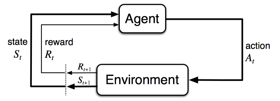
The environment transit and returns new $s_{t+1}, r_{t+1}$ to the agent, and agent needs to spit out a $a_t$ given a state $s_t$.
The previous section considers first learnig an action-value function $Q_\theta(s,a)$ and then using it to find the optimal policy $\pi_\theta(a\vert s)$, e.g. doing greedy/epsilon-greedy policy, e.g. learn a $Q$ using MC, TD, SARSA, etc.
can we perhaps directly learn a policy $\pi(a\vert s)$?
- though we often still need some estimate of $Q$ to do policy improvement, but we can avoid doing $\arg\max$ over all actions to get a policy
Advantages
- now action probability changes more smoothly, meaning better convergence
- easly for encoding exploratoin
- avoid the need of $\arg\max q(s,a)$ which can be costly if $\vert S\vert \times \vert A\vert$ is large
Disadvantages
- value-based could more efficient for a small number of states and actions
- hard to get an unbiased estimate through sampling (you will see that the gradient has an expected value term)
- many current approaches are still based on MC, hence many has high variance and could lower convergence speed
Policy Objective Functions
The first thing is to design an objective function to minimize. Note that we do not know a true policy but only an environment
- for $Q$/$V$ estimates, we can easily compute a loss from a target such as $r+\gamma Q$
Approaches: we need some measure (a single score $\in \mathbb{R}$) of how good a policy then:
-
in episodic environments, we can use the value function of the start state
\[J_1(\theta) = V^{\pi_\theta}(s_0) = \mathbb{E}_{\pi_\theta}[v_1]\] -
in continuing environments, we can use the expected return (which is the average of all possible returns)
\[J_{avV}(\theta) = \sum\limits_{s} d^{\pi_\theta} (s) V^{\pi_\theta}(s)\]which is basically the average of all possible returns, where $d^{\pi_\theta}(s)$ is the state distribution of the states under the policy $\pi_\theta$
-
in general, we can also use an average reward per time-step:
\[J_{avR}(\theta) = \sum\limits_{s} d^{\pi_\theta} (s) \mathbb{E}_{\pi_\theta}[r] = \sum\limits_{s} d^{\pi_\theta} (s) \sum\limits_{a} \pi_\theta(a|s) \mathcal{R}_s^{a}\]
and our aim is to maximize them. Given this, we now need to do gradient ascent:
\[\Delta \theta = \alpha * \nabla_\theta J(\theta)\]and no minus sign in front. But what is this gradient?
- to perform back-propagation, you need to have a derivative form of each operation = backed by math equation
- but considering the gradient above it is unclear what to do with the distribution of states $d^{\pi_\theta}(s)$ is also parameterized by $\theta$
Policy Gradient Theorem
Aim: manipulate the expression of gradient so that it does not need to do the summations
In a single step MDP problem we can fix the distribution of states:
\[\begin{align*} \nabla J(\theta) &= \nabla \sum\limits_{s} d^{\pi_\theta} (s) \sum\limits_{a} \pi_\theta(a|s) \mathcal{R}_s^{a} \\ &= \sum\limits_{s} d^{\pi_\theta} (s) \nabla \sum\limits_{a} \pi_\theta(a|s) \mathcal{R}_s^{a} \\ &= \sum\limits_{s} d^{\pi_\theta} (s) \sum\limits_{a} \nabla \pi_\theta(a|s) \mathcal{R}_s^{a} \\ &= \sum\limits_{s} d^{\pi_\theta} (s) \sum\limits_{a} \pi_\theta(a|s) \frac{\nabla \pi_\theta(a|s) }{ \pi_\theta(a|s) } \mathcal{R}_s^{a}\\ &= \sum\limits_{s} d^{\pi_\theta} (s) \sum\limits_{a} \pi_\theta(a|s) \underbrace{\nabla \ln \pi_\theta(a|s) }_{\text{score function} } \mathcal{R}_s^{a}\\ &= \sum\limits_{s} d^{\pi_\theta} (s) \mathbb{E}_{\pi_\theta}[\nabla_\theta \ln \pi_\theta(a|s) \mathcal{R}_s^{a}] \end{align*}\]Overall (proof in the book), the theorem looks like:
Policy Gradient Theorem: we can estimate the gradient for any differentiable policy $\pi_\theta$ and for any policy objective functions $J=J_1, J_{avR}$ or $\frac{1}{1-\gamma} J_{avV}$
\[\begin{align*} \nabla_\theta J(\theta) &= \nabla_\theta \sum\limits_{s} d^{\pi_\theta} (s) \sum\limits_{a} \pi_\theta(a|s) Q^{\pi_\theta}(s,a) \\ &\propto \sum\limits_{s} d^{\pi_\theta} (s) \sum\limits_{a} Q^{\pi_\theta}(s,a) \nabla_\theta \ln \pi_\theta(a|s) =\mathbb{E}_{s \sim \pi_\theta} \left[ \sum\limits_{a} Q^{\pi_\theta}(s,a) \nabla_\theta \ln \pi_\theta(a|s) \right] \end{align*}\]so that gradient does not flow through distribution $d$! note that the proportional up to a constant is fine because that can be absored into the learning rate $\alpha$
Example: gradient of Softmax policy using linear function approximation
Consider an naive modelling of $\pi$:
\[\pi_\theta(s,a) = x(s,a)^T \theta\]but recall that $\pi \in [0,1]$, yet this does not satisfy such a constraint. Hence we can consider
\[\pi = \mathrm{softmax}(x(s,a)^T \theta)\]for $\theta$ is a vector here. In this specific case, the score function of this form can be further computed as
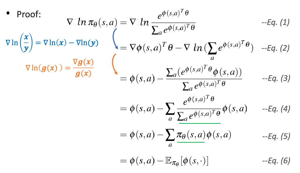
and you can use it do the policy gradient.
However, what if your action is continous? For a continous probability, prob is zero given a state/action. Therefore, we need to instead model a PDF:
\[a \sim \mathcal{N}(\mu(s), \sigma^2), \quad \mu(s) = x(s,a)^T \theta\]essentially modelling the mean to be modelled using VFA, and variance can either be pre-defined or also parametrized.
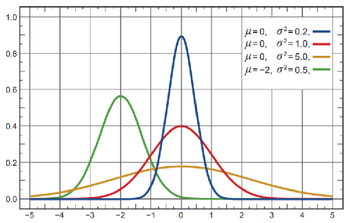
where each state has its own distribution, and the x-axis is the available actions you can take. Now, we can choose which action to take given a state we are at by sampling from the distribution.
Finally, in this case the score function is:
\[\nabla_\theta \ln \pi_\theta(a|s) = \frac{a-\mu(s)}{\sigma^2} x(s,a)\]MC Policy Gradient (REINFORCE)
Now we have already learned:
- objective function for policy
- gradient ascent methods
- can compute gradient using gradient theorem
- also specific forms if policy being softmax or Gaussian if continous
Recall that by policy gradient theorem:
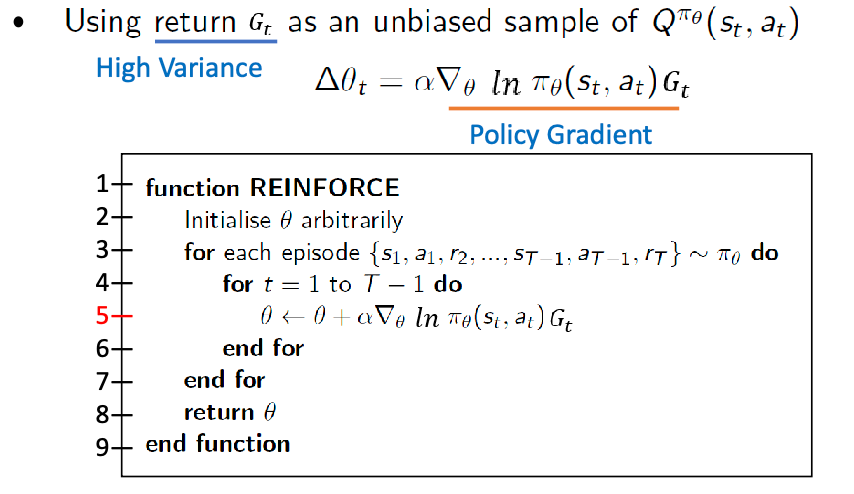
\[\nabla J(\theta) \propto \mathbb{E}_{s \sim \pi_\theta} \left[ \sum\limits_{a} Q^{\pi_\theta}(s,a) \nabla_\theta \ln \pi_\theta(a|s) \right]\]Reinforce: MC policy gradient method considers
\[\Delta \theta_t = \alpha \nabla_\theta \ln \pi_\theta(A_t|S_t) G_t\]
- use return $G_t$ as an unbiased estimator of $Q^{\pi_\theta}(s,a)$
- use one state $S_t$ and action $A_t$ to estimate the gradient
- therefore stochastic gradient ascent and consider
and the algorithm looks like:
Actor-Critic Methods
Aim: as MC methods using $G_t$ have a high variance, we can perhaps directly estimate $Q^{\pi_\theta}(s,a)$ and use it to estimate the gradient
- this can also tell you how good is the new policy/improved
Use a critic to estimate the action-value function:
\[Q_w(s,a) \approx Q^{\pi_\theta}(s,a)\]So we can directly compute the policy gradient:
\[\nabla J(\theta) \propto \mathbb{E}_{s \sim \pi_\theta} \left[ \sum\limits_{a} Q_w(s,a) \nabla_\theta \ln \pi_\theta(a|s) \right]\]Therefore Actor-Critic methods are:
- Critic: update action-value function parameters $w$ (e.g. using TD(0) or TD($\lambda$), basically our previous section on VFA)
- Actor: update policy parameters $\theta$ using policy gradient suggested by critic
Finally we approximate the policy gradient by stochastic sampling:
\[\Delta \theta = \alpha \nabla_\theta \ln \pi_\theta(A_t|S_t) Q_w(S_t,A_t)\]An example using TD(0)-based estimate of Q, the Actor-Critic Algorithm looks like
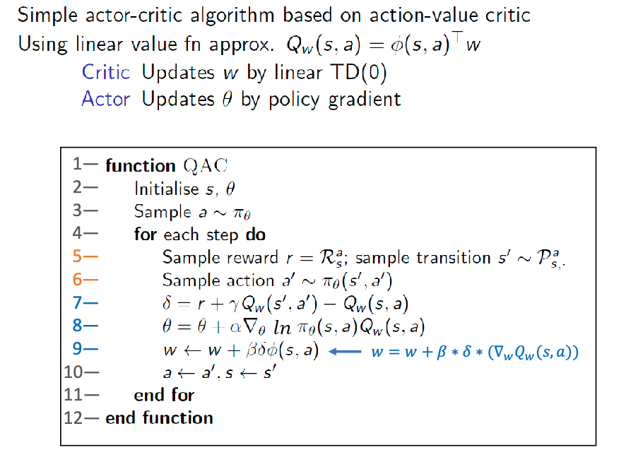
where basically:
-
line 5, 6 is data collection through interaction
-
line 7 is TD error and with line 9 for improving the critic (derived from gradient descent of MSE objective)
-
line 8 is policy gradient update
Compatible Function Approximation Theorem
A problem with actor-critic methods above is that approximating the policy gradient could introduce bias.
But it turns out that if we can choose VFA carefully, we can avoid introducing any bias
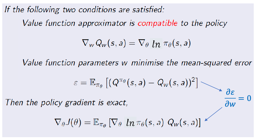
(proof skipped)
Policy Gradient with Advantage Function
Aim: we can reduce the variance of this existing policy gradient:
\[\nabla_\theta J(\theta) \propto \mathbb{E}_{s \sim \pi_\theta} \left[ \sum\limits_{a} Q^{\pi_\theta}(s,a) \nabla_\theta \ln \pi_\theta(a|s) \right]\]because variance could come from how you estimate $Q^{\pi_\theta}(s,a)$, and the stochastic sampling of $S_t$ and $A_t$. This can be done by subtracting the baseline:
\[Q^{\pi_\theta}(s,a) \to Q^{\pi_\theta}(s,a) - b(s)\]so that intuitively, picking $b(s)=V(s)$ can “re-center” all the $Q^{\pi_\theta}(s,a)$ and therefore reduce the variance
However, we could like our performance to still be unbiased, and it can be shown that this holds as long as baseline $b(s)$ a function not of $a$.
Proof: Consider the new gradient:
\[\nabla \ln \pi_\theta (s,a) * [Q_w(s,a) - B(s)]\]we want to make sure the gradient is the same as the original one, therefore, $\mathbb{E}[\nabla \ln \pi * B(s)] = 0$ needs to be proved.
By definitino of expectation
\[\begin{align*} \mathbb{E}_{s\sim \pi_\theta}[\nabla \ln \pi_\theta(s,a) * B(s)] &= \sum\limits_{s} d(s) \sum\limits_{a} \pi_\theta(a|s) \nabla \ln \pi_\theta(s,a) * B(s) \\ &= \sum\limits_{s} d(s) \sum\limits_{a} \pi_\theta(a|s) \frac{\nabla \pi_\theta(a|s)}{\pi_\theta(a|s)} B(s) \\ &= \sum\limits_{s} d(s) \sum\limits_{a} \nabla \pi_\theta(a|s) B(s) \\ &= \sum\limits_{s} d(s) B(s) \nabla \sum\limits_{a} \pi_\theta(a|s) \\ &= 0 \end{align*}\]since $\sum \pi = 1$ is constant, therefore the last $\nabla$ is zero. Notice that this worked because $B(s)$ does not depend on action
What is a good $B(s)$ to choose? One example is to use $V(s)$, hence the advantage funtion
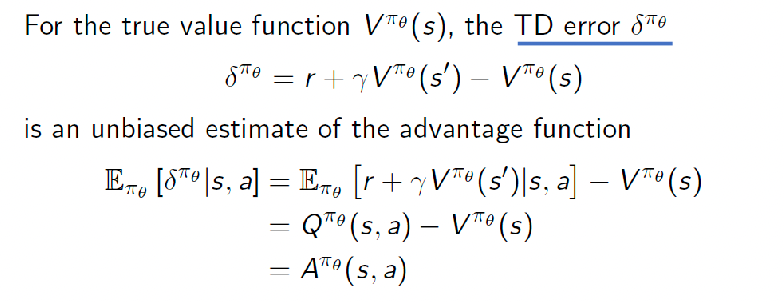
Policy Gradient with Advantage Function: the advantage function using $V(s)$ is:
\[A^{\pi_\theta}(s,a) = Q^{\pi_\theta}(s,a) - V^{\pi_\theta}(s)\]then the policy gradient is:
\[\nabla J(\theta) \propto \mathbb{E}_{s \sim \pi_\theta} \left[ \sum\limits_{a} A^{\pi_\theta}(s,a) \nabla_\theta \ln \pi_\theta(a|s) \right]\]
So how do we estimate the advantage function?
-
estimate both $V$ and $Q$ separately, need two more set of paramters
-
or we can estimate only using one (i.e. the value function)
so you only need to estimate $V$
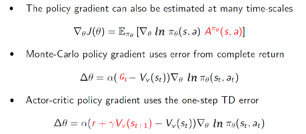
Actor and Critic at Different Time Scales
A final nuiances is that the we can vary how far ahead we look ahead by changing the time scale of actor and critic.
- critic: estimating the critic can use TD($0$) until $G_t$
- actor: estimating the actor can use different estiamte based on $V$
When estimating $Q$, we can also have actor at different time scales
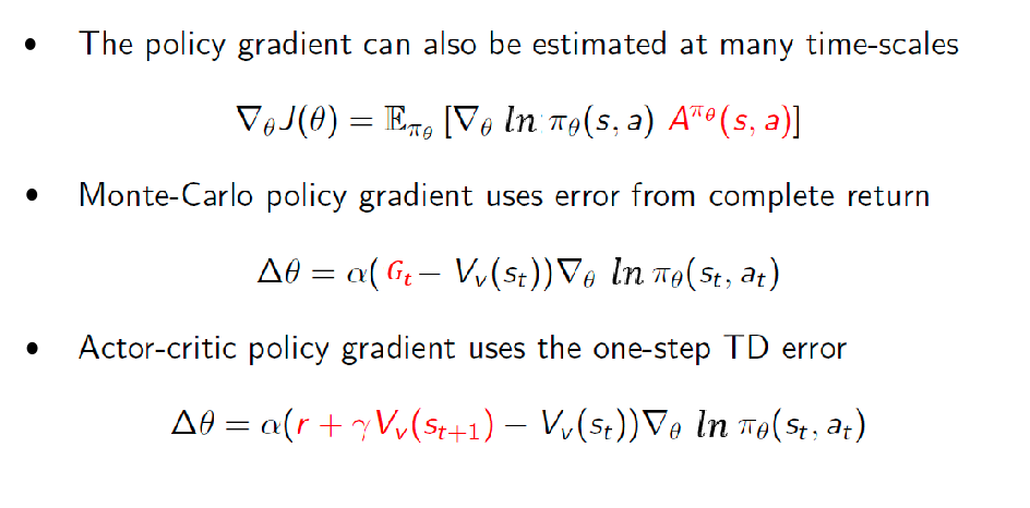
We estimating the policy gradient, if we have only a value estimate $V^{\pi_\theta}$:
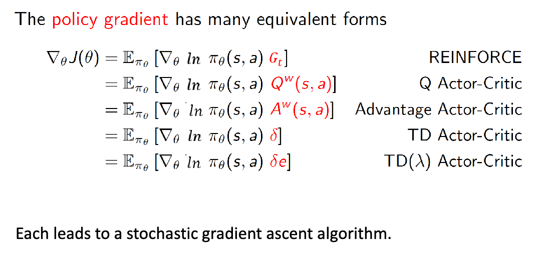
Summary of Policy Gradient Algorithms
Planning and Learning
Here, we shift focus back to the problem of planning/control. We consider situations where:
-
if you have access to a model, but your state/action space is enormous (DP is not a good idea), what is a good planning algorithm?
-
if you have enough data and you can fit a model reasonably well, how do you use it to further improve your planning algorithms (such as SARSA)?
-
in reality the convergence of model could be faster than fitting value/action function because the later needs information to propagate
-
but of course, fitting a model is not an easy task
-
Model-based methods rely on planning as their primary component, while model-free methods primarily rely on learning.
- Model-based: DP, and MCTS (this chapter). Also called the problem of planning
- Model-free: Q-learning, SARSA, etc. Also called the problem of learning
Of course, there are also hybrids, so that you can use a model/learned model to improve model-free algorithms, such as Dyna (this chapter)
Rollout Algorithms and Tree Search
First, we discuss the model-based planning where model of the world is given.
For instance, consider the rule of Go game
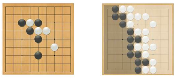
so that to plan each step, we need to think ahead. Therefore, it might make sense to consider simulation as part of planning: if I take this step here, what happens next and can I win? So rollout algorithms in general involve
- try all potentially high reward possibilities/moves starting from the current position
- estimate those moves=actions by simulation=rollout, and sometimes in combination with some value function estimate
- pick the best move (e.g. UCB), and repeat
Rollout algorithms are decision-time planning algorithms based on Monte Carlo control applied to simulated trajectories that all begin at the current environment state.
- They estimate action values for a given policy by averaging the returns of many simulated trajectories that start with each possible action and then follow the given rollout policy.
- When the action-value estimates are considered to be accurate enough, the action (or one of the actions) having the highest estimated value is executed, after which the process is carried out anew from the resulting next state.
This is also important as we talk about the details of an rollout algorithm: MCTS, which is that
It can be said the aim of a rollout algorithm (e.g. MCTS) is to improve upon the rollout policy; not to find an optimal policy.
- In some applications, a rollout algorithm can produce good performance even if the rollout policy is completely random.
- But the performance of the improved policy depends on properties of the rollout policy and the ranking of actions (e.g. Upper Confidence Bound) produced by the Monte Carlo value estimates.
- Intuition suggests that the better the rollout policy and the more accurate the value estimates, the better the policy produced by a rollout algorithm (e.g. MCTS) is likely be (but see Gelly and Silver, 2007, and in AlphaGo it more human-like policy instead of better policy may be better).
Upper Confidence Bounds
Upper Confidence Bound: get a better balance between exploration and exploitation, besides e-greedy and softmax approach we have seen before.
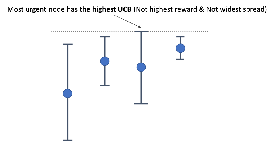
- e-greedy action selection forces the non-greedy actions to be tried, but indiscriminately, with no preference for those that are nearly greedy or particularly uncertain.
- It would be better to select among the non-greedy actions according to their potential for actually being optimal, taking into account both how close their estimates are to being maximal and the uncertainties in those estimates.
The ultimate form of the simple version of UCB looks like, for a one-step MDP problem (i.e. without states)
\[a_t = \arg\max_a \left[ Q_t(a) + c \sqrt{\frac{\ln n_t}{N_t(a)}} \right]\]where:
- $n_t$ is the total number of actions you have taken until time $t$, and $N_t(a)$ is the total number of times an action $a$ is taken up to time $t$
-
$Q_t(a)$ is your current estimated return of action $a$
- the $\arg\max$ is because we are doing the upper confidence bound
- essentially the left term is your exploitation, and right term is exploration trying to visit less-visited states
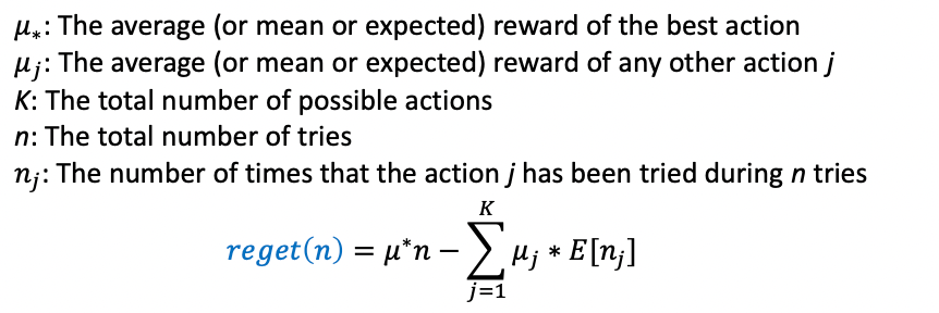
This form is derived from modeling the regret of each action you made, and minimize your regret.
What does this have to do with UCB?
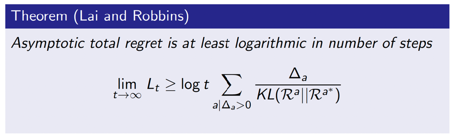
- Lai and Robbins showed that the regret for the multi-armed bandit has to grow at least logarithmically w.r.t. the number of plays $n$
- UCB is proved to grow the regret logarithmically in that case (by choosing actions from UCB), hence is optimal in that case
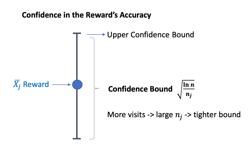
We can visualize what UCB is doing to be first estimating the “confidence” of your current estimate, and then pick the ones that are most promising
| Confidence Bound | Upper Confidence Bound Action |
|---|---|
 |
 |
But in reality, UCB might not be easy to work with. Consider a realistic problem where you could have a large state space:
\[a_t = \arg\max_a \left[ Q_t(s,a) + c \sqrt{\frac{\ln n_t}{N_t(s,a)}} \right]\]the $N_t(s,a)$ for many combinations will be zero until explored. Hence in those cases simple e-greedy of softmax could also work as well and is much simpler.
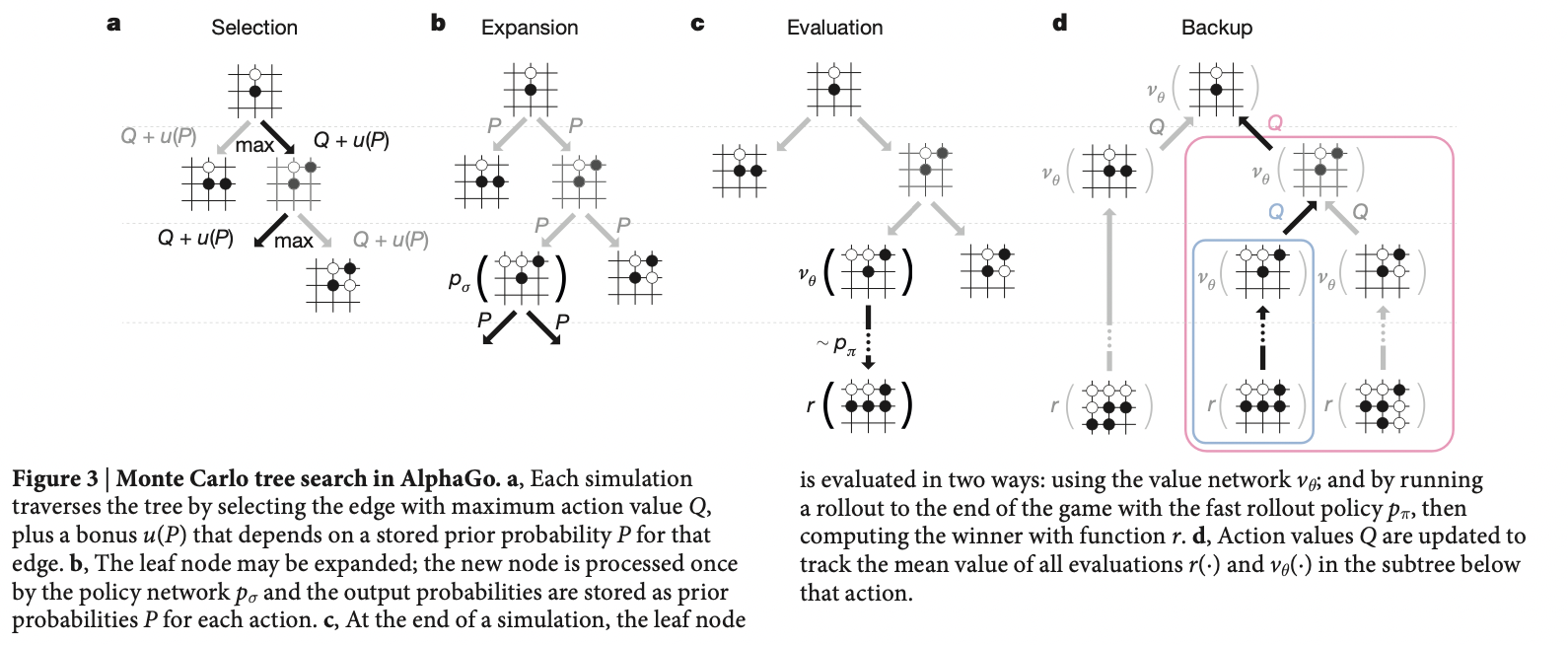
Monte Carlo Tree Search
Now we can talk about MCTS. The objective is to do planning given a model, and specifically to improve upon a rollout policy (by significant margin, e.g. improvement in computer Go from a weak amateur level in 2005 to a grandmaster level (6 dan or more) in 2015.)
At its base, MCTS is a rollout algorithm as described above, but enhanced by the addition of a means for accumulating value estimates obtained from the Monte Carlo simulations in order to successively direct simulations toward more highly-rewarding trajectories.
At its core, on high level the following is happening
- MCTS is executed after encountering each new state to select the agent’s action for that state; it is executed again to select the action for the next state, and so on.
- MCTS incrementally extends the tree by adding nodes representing states that look promising based on the results of the simulated trajectories
- Outside the tree and at the leaf nodes the rollout policy is used for action selections, but at the states inside the tree something better is possible. For these states we have value estimates for at least some of the actions, so we can pick among them using an informed policy, called the tree policy, that balances exploration (e.g. using UCB).
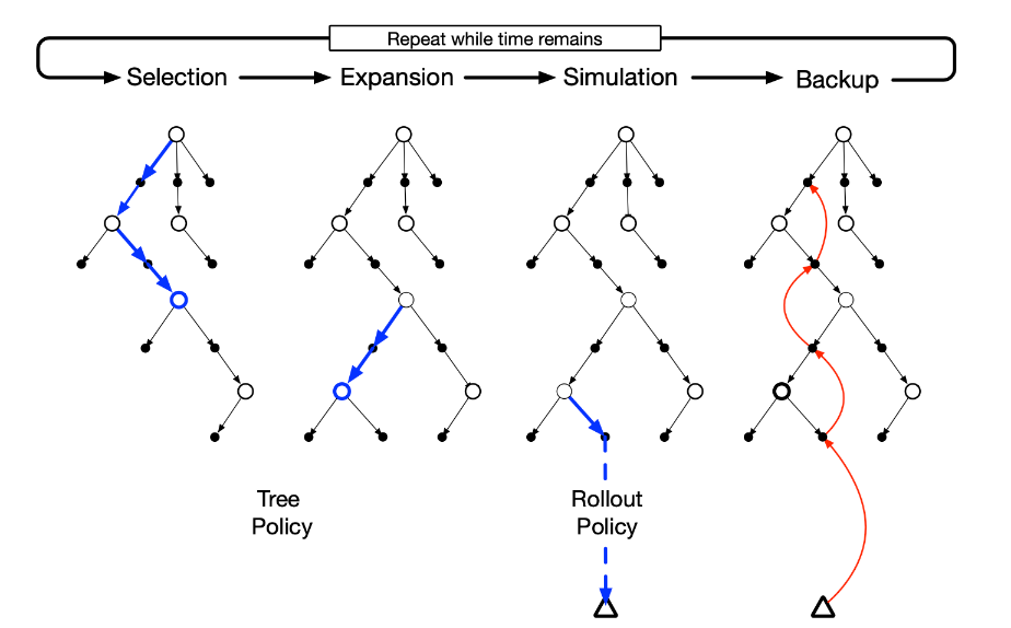
In more details and to explain what the above means, consider the overall algorithm iteratively performing
- MCTS continues executing these four steps, starting each time at the tree’s root node, until no more time is left
- Selection. Starting at the root node, a tree policy (e.g. UCB) based on the action values attached to the edges of the tree traverses the tree to select a leaf node
- Expansion. The tree is expanded from the selected leaf node by adding one or more child nodes reached from the selected node via unexplored actions
- Simulation. From the selected node, or from one of its newly-added child nodes (if any), simulation of a complete episode is run with actions selected by the rollout policy.
- The result is a Monte Carlo trial with actions selected first by the tree policy and beyond the tree by the rollout policy.
- Backup. The return generated by the simulated episode is backed up to update, or to initialize, the action values attached to the edges of the tree traversed by the tree policy in this iteration of MCTS. No values are saved for the states and actions visited by the rollout policy beyond the tree, as shown by the little triangle branch being dotted and discarded. Simulation result is only used to backup the existing tree
- basically update my estimates of how good each action is based on simulation (+ value estimate in AlphaGO)
- Then, finally, an action from the root node (=the current state of the environment) is selected according to some mechanism that depends on the accumulated statistics in the tree; for example, e.g. largest action value accumulated by UCB
- After the environment transitions to a new state, MCTS is run again from the first step (often starting with a tree containing any descendants of this node left over from the tree constructed by the previous execution of MCTS)
What does the accumulated estimate $Q(s,a)$ at each action node correspond to? In rollout algorithms where $s$ is the current state and $\pi$ is the rollout policy, averaging the returns of the simulated trajectories produces estimates of $q_\pi(s,a)$ for each action $a$.
Then the policy that selects an action in s that maximizes these estimates and thereafter follows $\pi$ (during simulation) is a good candidate for a policy that improves over $\pi$. The result is like one step of the policy-iteration algorithm of dynamic programming
- you will see in AlphaGO we can potentially do better to estimate $q_*(s,a)$ hence choose the optimal action instead of just improvement
For example: Let us be playing a game of GO. Let us say we have some tree already, and we would like to use UCB based on action value to be our tree policy to select a node
-
Selection:
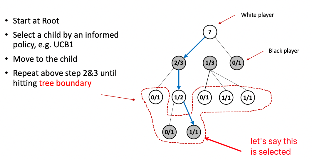
where here, we have already made 7 simulations/rollouts hence the top node stores 7.
-
the $2/3$ at black node (at second level) means it’s black’s turn to act, but after this white action white has won $2/3$ times in the simulation
-
if we are computing the UCB of each node for instance at the second level:
\[\mathrm{UCB}(2/3) =\frac{2}{3} + \sqrt{2} \sqrt{\frac{\ln 7}{3}}\]for using $c=\sqrt{2}$.
-
-
Expansion: we have selected a node and we want to explore some actions by adding a child node:
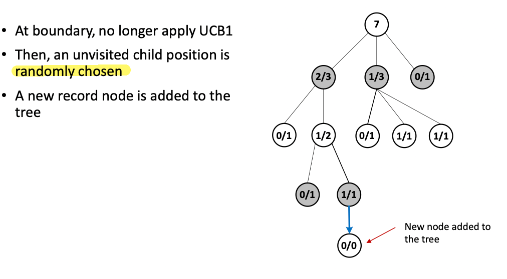
-
Simulation: we simulate from the newly added node using a rollout policy (e.g. a fast agent trained supervised from online GO games)
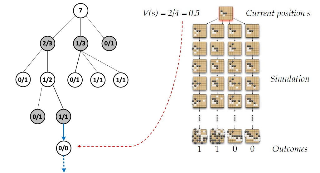
-
Back-Propagation: we discard the simulation trajectory but utilize the results to update our existing tree
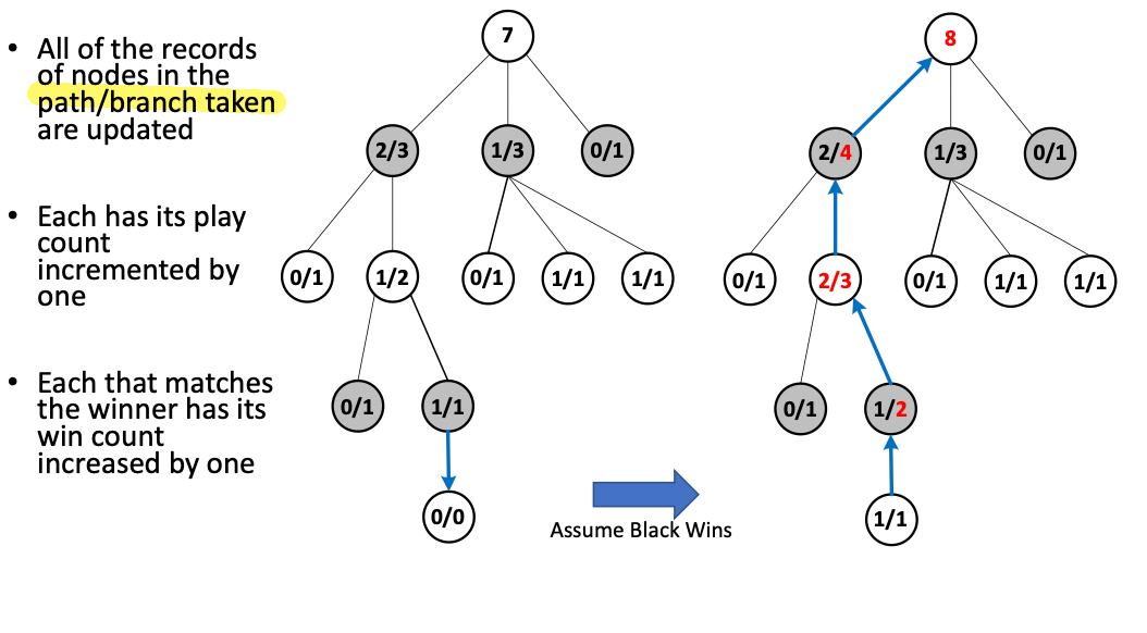
notice that all we need to update is the branch. (Recall that the white $1/1$ means its white’s turn but black has won $1/1$, hence the previous black node becomes $1/2$ as there are now in total $1+1=2$ simulations done and white lost one of them)
But of course, no algorithm is yet perfect:
| Pros | Cons |
|---|---|
| Tree growth focuses on more promising areas | Memory intensive: entire tree in memory |
| Can stop algorithm anytime to get search results | For complex problems, enhancement needed for good performance |
| Avoid the problem of globally approximating an action-value function (as in DP) | |
| Convergence to minimax solution | |
| High controllability = can insert your prior domain knowledge into tree policy, for instance |
AlphaGO
The famous AlphaGO in essence is a MCTS algorithm, but enhanced by several changes, e.g. make the GO simulation computationally fast using value functions.
The overall pipeline of AlphaGO involves:
-
train a supervised policy $p_\sigma$ cloning the plays of experts.
-
use policy gradient to train another agent $p_\rho$, which can consistently beats (more than 80% of the time) $p_\sigma$
-
obtain value function $V_\rho$ from the strongest player $p_\rho$, hoping that $V_\rho \approx V_*$ of the optimal play
-
use MCTS to play by
-
tree policy is UCB
-
expansion is done using the prior from $p_\sigma$, which is found to perform better than $p_\rho$ as the former is more diverse and human-like
-
backpropagation uses both simulation results and $V_\rho$, so that the value for each leaf node is
\[V(s_L) = (1-\lambda) v_\theta (s_L) + \lambda z_L\]and each edge/action is the mean evaluation of all simulations through that edge
\[Q(s,a) = \frac{1}{N(s,a)}\sum_{i=1}^n \mathbb{1}(s,a,i)V(s_L^i)\]so that $\mathbb{1}(s,a,i)$ indicates if the edge $(s,a)$ was traversed during the $i$-th simulation.
-
at the end of simulation/MCTS, play policy is to select action with most visited state:
\[a = \arg\max_{a} N(s,a)\]
-
more details see paper: https://www.nature.com/articles/nature16961
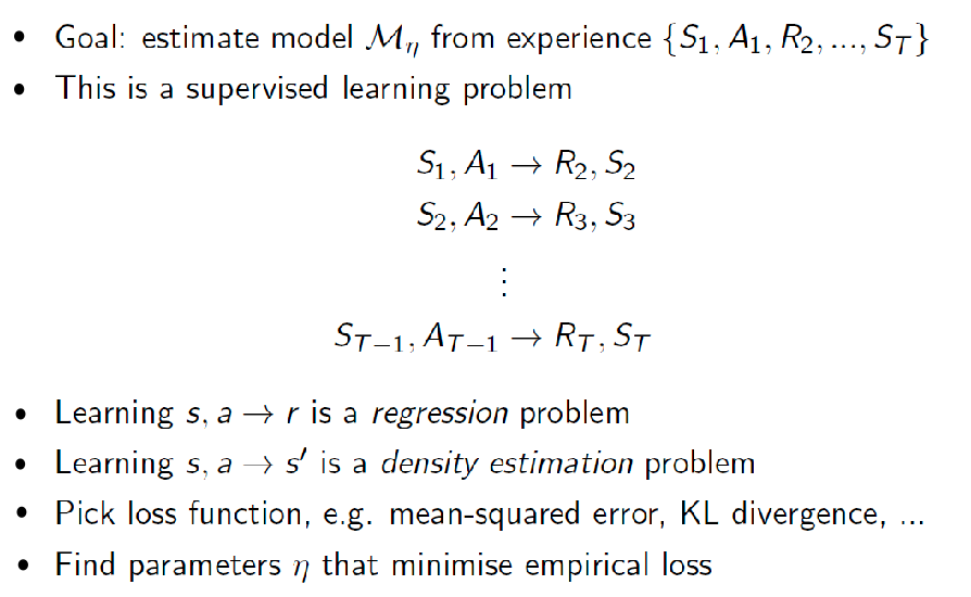
Sample-Based Planning
Now we have covered planning if given model: for small spaces DP can be gone, but more often MCTS which selectively expands search space is more tractable. However, what if we don’t know the model, i.e. model-free? Do we have to only use Q-learning/SARSA etc?
If model is unknown, we can first learn the model and then plan.
- once the model is fitted, we can do planning using DP, value iteration, policy iteration, MCTS, etc.
- or, we can use the model to generate more samples to fit $Q$ functions
Recall that for a model, we need to spit out next state and reward:
\[S_{t+1} \sim \mathcal{P}_\eta (S_{t+1}|S_t, A_t)\\ R_{t+1} \sim \mathcal{R}_\eta (S_{t+1}|S_t, A_t)\\\]for a model parameterized by $\eta$, and we typically can assume independence so that:
\[\mathbb{P}(S_{t+1},R_{t+1}|S_t, A_t) = \mathbb{P}(S_{t+1}|S_t, A_t)\mathbb{P}(R_{t+1}|S_t, A_t)\]This then would be useful when learning a distribution model.
Some models produce a description of all possibilities and their probabilities; these we call distribution models. Other models produce just one of the possibilities, sampled according to the probabilities; these we call sample models.
- e.g. consider modeling the sum of a dozen dice. A distribution model would produce all possible sums and their probabilities of occurring, whereas a sample model would produce an individual sum drawn according to this probability distribution.
For algorithms such as Q-learning and SARSA, we just need a sample model. But for DP, we would need a distribution model.
It is typically easier to learn a sample model, which can be done using supervised learning
For Example: Small Table Lookup Example.
For small state spaces, you can learn a distribution model by simply counting:
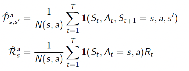
So in the case of the following experience/data, you can easily fit a distribution model:
| Experience | Model Learned |
|---|---|
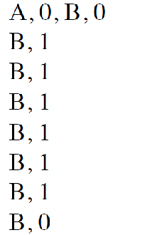 |
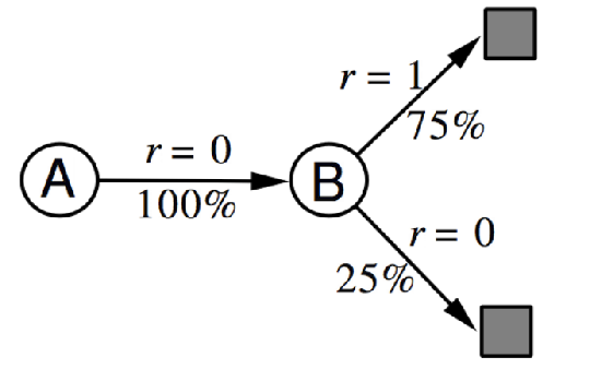 |
in this case we calculated the model without supervised learning but directly computing, but the idea is the same.
Then, once we have a model, we can sample from it to do MC control, for instance:
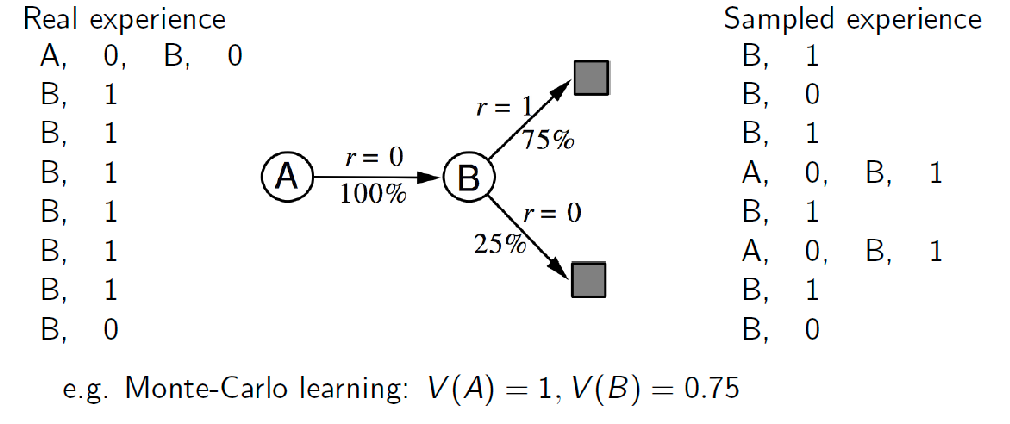
Or of course, we can plan given a model directly by doing DP or MCTS.
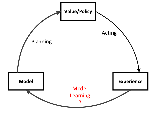
Integrating Learning and Planning
There is also an approach to try to do learning and planning:
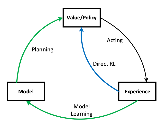
Within a planning agent, there are at least two roles for real experience:
- model-learning: it can be used to improve the model (to make it more accurately match the real environment)
- direct RL: it can be used to directly improve the value function and policy using the kinds of reinforcement learning methods we have discussed
Note how experience can improve value functions and policies either directly or indirectly via the model. It is the latter, which is sometimes called indirect reinforcement learning, that is involved in planning.
An example algorithm is Dyna-Q: which combines Q-learning and model learning as shown below
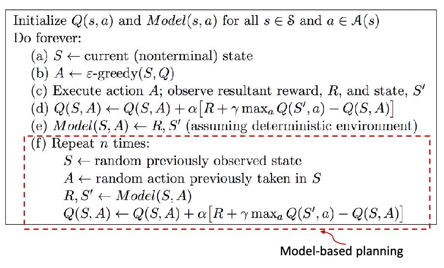
notice that step a)-d) is basically Q-learning, and step e)-f) further update your Q function using the model
-
the intuition is that if you can explore more from your previous $(S,A)$, you could make better decisions sooner in the future when you met similar states, whereas just doing Q-learning makes that part slower
-
For instance, as you can see here the more simulated experienced you gave to Q, it makes better decisions earlier and hence converge faster. i.e. While walking around the world according to the experience, I am changing dynamically/planning at each step as well
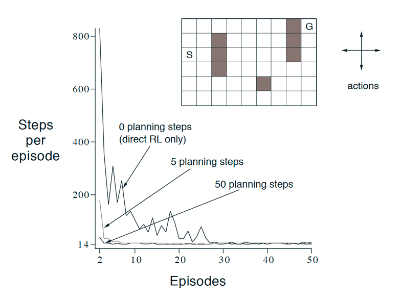
the idea of updating a bit sooner than until the end is like TD v.s. MC.
Unified View of Planning and Learning
Just like how we Generalized Policy Iteration to contextualize model-free algorithms, the overall framework of planning and learning also shares high level similarity. The unified view we present in this chapter is that all state-space planning methods share a common structure

- all state-space planning methods involve computing value functions as a key intermediate step toward improving the policy, and
- they compute value functions by updates or backup operations applied to simulated experience.
Deep Reinforcement Learning
Deep L can model any components in RL such as policy, model, value function, but Deep L + RL is unstable and hard to get convergence
Current approaches, modeling:
- value-based RL
- approximating value function $Q^$ or $V^$ using a NN with weight $w$ or $\theta$
- e.g. Q-learning, SARSA, MC methods, TD methods, etc.
- policy-based RL
- search for and approximate the optimal policy function $\pi^*$
- stochastic policy = policy model outputs a distribution of actions (e.g. by Softmax, or Gaussian distribution), and then you sample from it
- deterministic policy = find a function that gives the action directly
- model-based RL
- build a model (transition function and reward) from samples
- when obtained a model, do planning
DL for Value Functions
Here we will discuss on algorithm that has been successful and can be used for control (by simply taking $a = \arg\max_a Q(s,a)$)
Deep Q-Network (DQN)
As we have mentioned before, this aims to model the Q network
\[Q(s,a,w)\approx Q^\pi (s,a)\]and your target is simply based on the Q-learning target, which gives you a loss function:
\[\mathcal{L}(w) = \mathbb{E}\left[ \left( \underbrace{r+\gamma \max_{a'} Q(s',a',w)}_{\text{target}} - Q(s,a,w) \right)^2 \right]\]notice that you need to forward pass twice for $(s,a)$ and $(s’,a’)$.
-
Could there be some correlation there? Keep that in mind
-
note that $a’$ will be computed by the 1) can model $Q(s,a) \to \mathbb{R}^{\vert A\vert }$ and then index into the action $a$ to get the $Q$ value. 2) then in this method, picking $\arg\max Q$ can be one using only one forward pass
then you perform gradient descent, which would look like the same descent in Q-learning
\[\frac{\partial \mathcal{L}(w)}{\partial w} = \mathbb{E}\left[ \left( r+\gamma \max_{a'}Q(s',a',w)-Q(s,a,w) \right) \frac{\partial Q(s,a,w)}{\partial w} \right]\]However, naive Q-learning oscillates or diverges with neural nets
- data is sequential, hence there are correlations between successive samples
- policy could change rapidly with slight change in $Q$-values
- correlation between $Q$-value and target value during the loss computation
- scale of rewards and $Q$-values could vary and hence gradient might be unstable
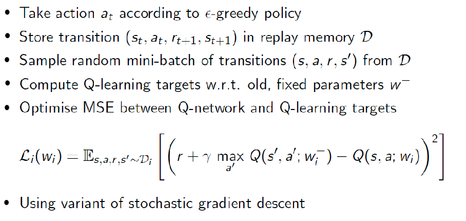
There are the core issues that DQN attempts to solve:
DQN provides a stable solution to deep value-based RL
- experience replay to break correlation in data/experience
- freeze target $Q$-network (periodically, for example update only after 10k steps) to break correlations between $Q$-network and target, and avoid policy changes too rapidly
- clip or normalize reward so network can work adaptively to ranges of Q-values = robust gradients
Therefore the algorithm below
DL for Policy Functions
Here we aim to directly learn a policy, and we will cover methods such as
- Actor-critic methods: DDPG, A3C
- Optimization methods: TRPO, GPS
In general, policy gradient based methods are quite popular today, especially when continuous action spaces.
Deterministic Policy Gradient
Recall that during stochastic policy approximation, we considered modeling the (real) policy:
\[\pi_\theta(a|s) \to \mathbb{P}[a|s;\theta]\]where we could do this by taking a Softmax of the output, or modeling parameters of a Gaussian distribution for continuous action space. But here, we might consider a deterministic policy:
\[\mu_\theta(s)\to a\]Why does this matter? As $\mu_\theta$ is the network, and it no longer models a probability the stochastic policy gradient theorem we had before (using probability):
\[\nabla J(\theta) \propto \mathbb{E}_{s \sim \pi_\theta} \left[ \sum\limits_{a} Q^{\pi_\theta}(s,a) \nabla_\theta \ln \underbrace{\pi_\theta(a|s)}_{\text{prob.}} \right]\]no longer makes sense as using $\ln \mu_\theta(s)$ does not make sense any more. Therefore, people proved that there is a policy gradient for deterministic case:
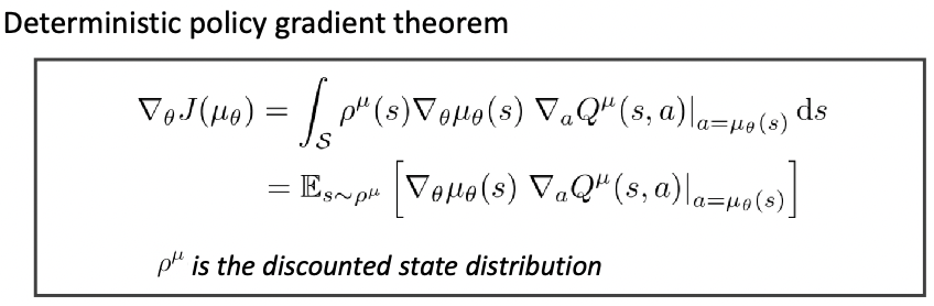
where the objective function in this case would be:
\[J(\theta) = \mathbb{E}[r_1 + \gamma r_2 + \gamma^2 r_3 + ....] = \mathbb{E}_{\mu_\theta}[G]\]basically the expected return if we follow policy $\mu_\theta$
But why use/prefer deterministic policy? Difference in practice?
when the variance in stochastic tends to zero, it became the deterministic case
- stochastic needs gradient descent in $\mathbb{E} [\nabla \pi_\theta(s,a)*G_t ]$, meaning we for a single state we need action spaces combined for a good estimate v.s. deterministic case in practice needs only to scan over a much smaller actions
- therefore can outperform significantly when action space is high dimensional
stochastic encourages more exploration as in the end you are sampling from the distribution v.s. deterministic policy might not explore other possibilities. For instance
\[a = \mu_\theta(s) + \text{Noise}\]so then all your exploration is the noise term
Deep Deterministic Policy Gradient
The overall idea is basically combining DL + DPG + Actor Critic Method by:
- use actor-critic method to compute DPG gradient
- model your actor and critic using deep learning
- (solve instability issues with soft updates)
Therefore, first we consider modeling a policy/actor with DL:
\[a = \pi(s,u)\]with weights $u$, and a critic network $Q(s,a,w)$ with weights $w$. Then the gradient updates are simply:
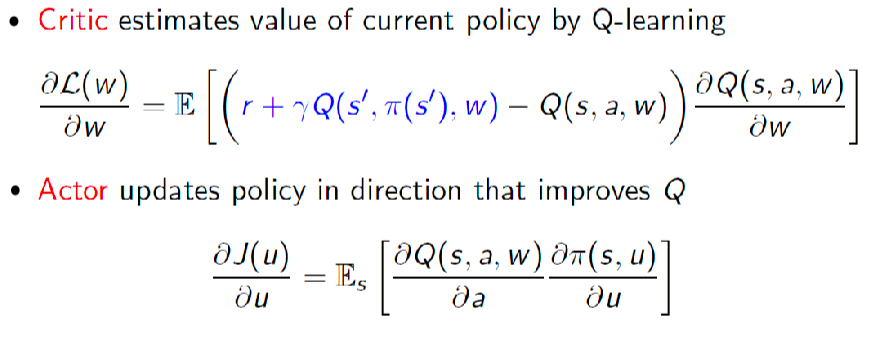
so in total here we have two networks, where the critic update is basically no $\max$ version of DQN updates, then use that to calculate gradient for actor
Again, naive actor-critic method oscillates or diverges with neural network
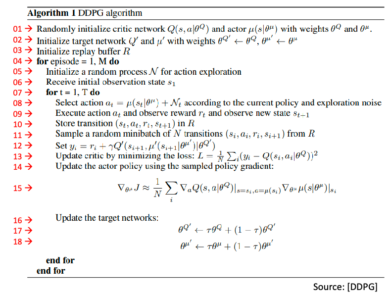
Then in DDPG, we use
-
experience replay as in DQN for both actor and critic
-
four networks where soft target update is used instead of freezing
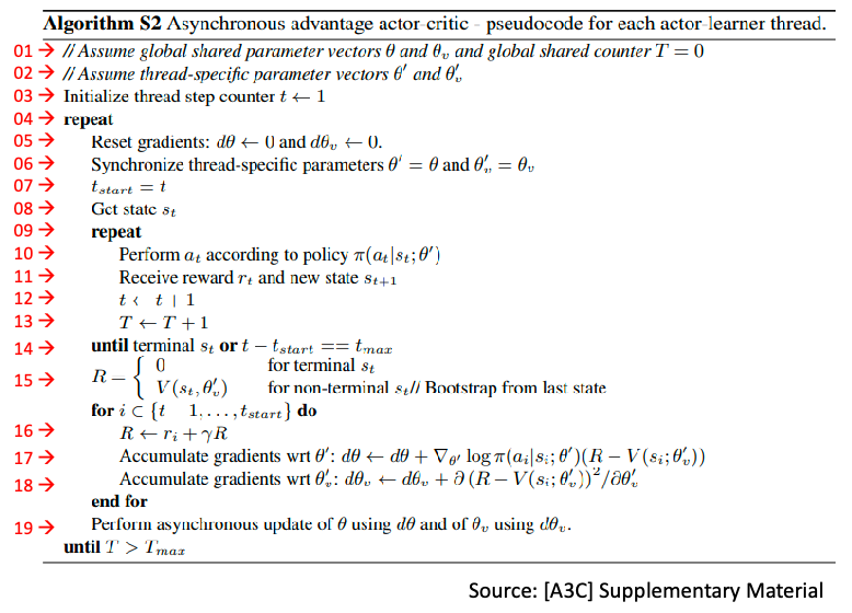
Asynchronous Advantage Actor-Critic (A3C)
Again, building on top of actor-critic method but being
- Asynchronous: initiate multiple agents, each interact with the environment independently, and report update back to global network
- Advantage: using advantage function instead of $Q$ to update policy
Therefore overall it looks like:
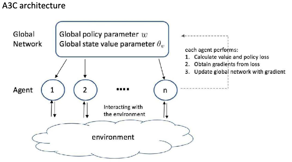
So in a sense data correlation is removed automatically because each agent has independent interactions = no need to maintain an experience buffer.
The overall algorithm then looks like:
Why A3C over other actor-critic methods?
- naturally has decoupled correlation, v.s. in DQN and DDPG an experience buffer is used
- runs many agents in parallel to collect samples for updates, hence fast in computing/updates as well
- each agent can use different exploration policy, which can maximize diversity and further decorrelate
- can run on multi-core CPU threads on a single machine to reduce communication overhead
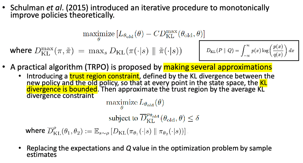
Trust Region Policy Optimization (TRPO)
Basically a new form of loss function/objective, other than the simple ones such as $J(\theta)=\mathbb{E}{\mu\theta}[G]$
DL for Model Functions
Now, we can also use a model to learn the world model, i.e. the transition functions
\[p(r,s'|s,a)\]so that after this, we can:
- use it to collect more data and improve value function estimates
- do planning directly, such as MCTS
AlphaGo Zero
Recall that the first version AlphaGO, we used
one network for roll-out policy, another for SL policy, both from human data
- self-play to improve policy network: learn a RL policy network and a value network as well
- MCTS based on the tree policy (RL network) and UCB
- expand using rollout policy and combine with value function
- pick action based on UCB
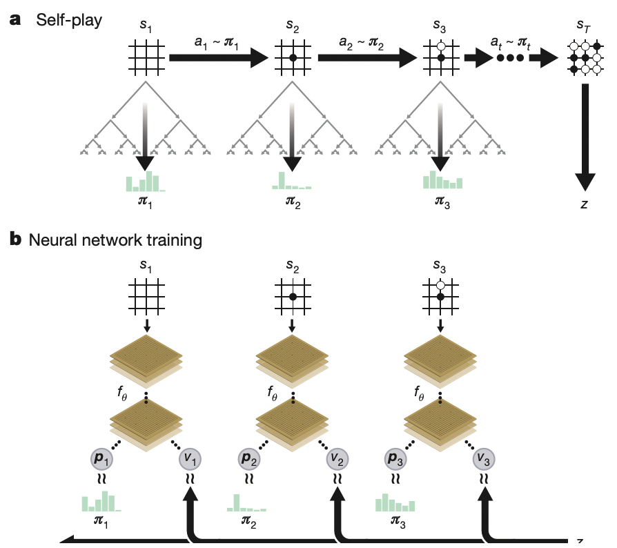
For AlphaGo Zero, the emphasis is to learn without human knowledge entirely. The core idea is that it is solely based on reinforcement learning and MCTS to improve.
-
start with a single model producing both the move probability/policy and the value function
\[f_\theta(s) = (p_\theta(a|s), V_\theta(s))\] -
since the model does not care which player you are, it can self-play. But additionally, here we consider self-play using MCTS instead of just the policy $f_\theta$ because MCTS can usually result in selecting a much stronger move, hence an be treated as a policy improvement operator
-
Then, we have effectively gathered $(\pi,z)$, where $\pi$ is the MCTS probability and $z$ is the game winner. This game winner $z$ can be seen as a policy evaluation operator, which we can use to improve $V_\theta(s)$ estimate as well.
-
but how exactly do we model $\pi$ probabilities in the MCTS? AlphaGo Zero models this to be:
\[\pi_a \propto N(s,a)^{1/ \tau}\]so that the more popular a move is the higher the probability. Then how does it select those moves?
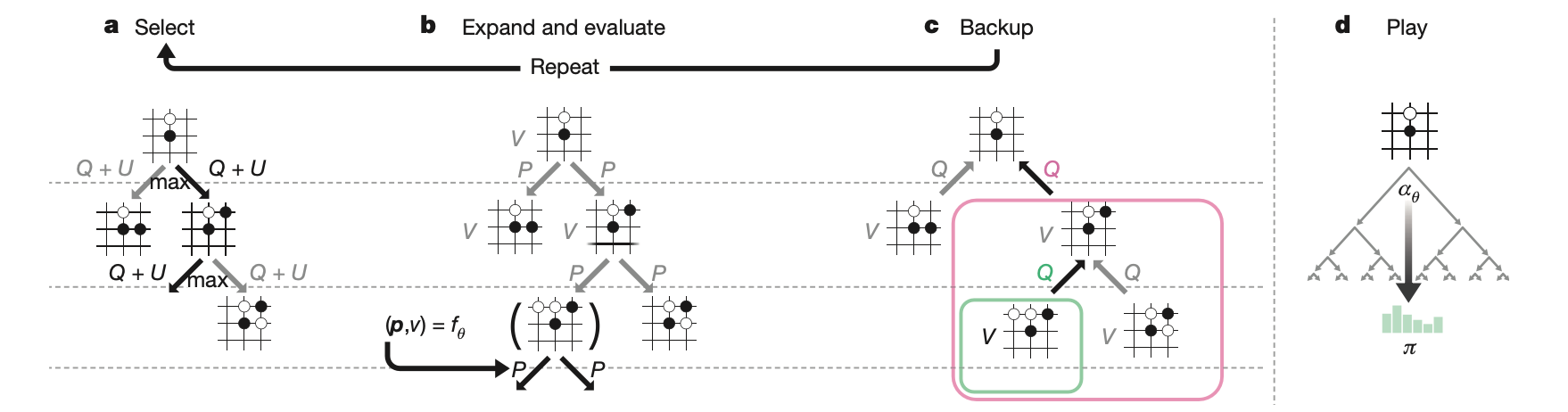
essentially it uses $f_\theta$ to help expand the tree so that each edge stores the $P(s,a),N(s,a),Q(s,a)$ where
- each simulation step selects a move that maximizes upper confidence bound $Q(s,a)+U(s,a)$, where $U(s,a)\propto P(s,a)/(1+N(s,a))$ until a leaf node is encountered. This basic form is also used in Alpha Go
- the leaf node is then evaluated and expanded only once using the prior probability and value $(P(s’,\cdot), V(s’) = f_\theta(s’))$. Notice no rollout here!
- each edge $(s,a)$ traversed is then updated to increment its visit count $N(s,a)$ and its action value to be the mean evaluation $Q(s,a)=\sum V(s’)/N(s,a)$.
- once done, a winner $z={+1,-1}$ is stored, and the MCTS probability $\pi_a$ is computed
-
Finally, you have basically had a improved policy and value $(\pi,z)$, you update your network to match those parameters to achieve policy improvement and policy evaluation
\[\mathcal{L}=(z-v_\theta)^2 - \pi^T \log p_\theta + c||\theta||^2\]where the last term is simply a regularization.
-
Note that at the end of training/during actually play, you also perform the same MCTS procedure above and select move based on the play policy $\pi$
Note that some key difference with Alpha Go include
learn RL network + value network during self-play from scratch without human knowledge
modified MCTS to
use value network without roll-out
modified UCB $\mathrm{UCB}(s,a)=Q(s,a)+U(s,a)$, where $U(s,a)\propto P(s,a)/[1+N(s,a)]$
final play policy $\pi$ becomes stochastic (is not the tree policy which is UCB)
\[\pi(a|s) = \frac{N(s,a)^{1/\tau}}{\sum_b N(s,b)^{1/\tau}}\]which is then used to instruct the model $p_\theta$ to achieve policy improvement.
And just to re-iterate the key aspects in the paper (borrowing the author’s words)
The AlphaGo Zero selfplay algorithm can similarly be understood as an approximate policy iteration scheme in which MCTS is used for both policy improvement and policy evaluation.
- Policy improvement starts with a neural network policy, executes an MCTS based on that policy’s recommendations, and then projects the (much stronger) search policy back into the function space of the neural network.
- Policy evaluation is applied to the (much stronger) search policy: the outcomes of selfplay games are also projected back into the function space of the neural network. These projection steps are achieved by training the neural network parameters to match the search probabilities and selfplay game outcome respectively.
Other RL Topics
There are many other topics of RL we haven’t discussed, including:
- various other methods for balancing exploration and exploitation
-
Federated Reinforcement Learning, e.g. using edge devices
- Multi-agent Reinforcement Learning.
- Recent breakthrough achieving human level performance in Stratego, “solving” incomplete information problem
More on Exploration and Exploitation
Online decision has a fundamental trade-off between exploration and exploitation. Here we want to discuss various different schemes that you can use to balance such as trade-off
- e.g. MCTS contains search using tree policy = exploitation, but expands using UCB, which helps exploration
Some design principles for exploration include
- Naive Exploration. e.g. DDPG adding noise to a policy for exploration
- Optimistic Initialization: initialize $\hat{Q}$ to be larger than expected reward in the beginning
- Optimistic in the face of uncertainty: UCB as an example
- compute uncertainty over time, and prefer actions with uncertain values for exploration
- Probability Matching: choose action according to some “model” you have about the reward distribution
- Information state search: lookahead search
For many examples below, we will assume a Multi-arm Bandit problem, meaning there will be no state for simplicity
Optimistic Initialization
One very simple and practical idea to guarantee exploration is to initialize $Q(a)$ to be high(er than expected reward). So that:
- for actions that perform lower than that, we automatically explore other actions
In practice, we can do this by:
-
initialize high $Q$
-
Update action value by incremental MC evaluation
\[\hat{Q}_t(a_t) = \hat{Q}_{t-1} + \frac{1}{N_t(a_t)}(r_t - \hat{Q}_{t-1})\]
However, this can still lock onto sub-optimal actions over time, as you will see later that both greedy/$\epsilon$-greedy + optimistic initialization will have linear total regret.
Regret
Recall that regret aims to measure the opportunity loss, which can be measured by the difference between the optimal and your chosen action.
\[l_t = \mathbb [ V^* - Q(a_t)]\]then the total regret over time is
\[L_t = \mathbb{E} \left[ \sum_{\tau=1}^t V^* - Q(a_\tau) \right]\]so minimizing regret = maximize cumulative reward
But regret can then be reformulated using the gap $\Delta_a = V^*-Q(a)$ for every action:
\[\begin{align*} L_t &= \mathbb{E} \left[ \sum_{\tau=1}^t V^* - Q(a_\tau) \right]\\ &= \sum_{a \in \mathcal{A}} \mathbb{E}[N_t(a)] (V^* - Q(a)) \\ &= \sum_{a \in \mathcal{A}} \mathbb{E}[N_t(a)] \Delta_a \end{align*}\]So for a good algorithm, we want to
- have large $N$ for small $\Delta_a$, and vice versa to minimize this (of course you need to get an accurate measure of $\Delta_a$ first)
- idea is so that you would want to choose that small $\Delta_a$ action over and over.
How does some simple approach perform in this metric? For multi-arm bandit:
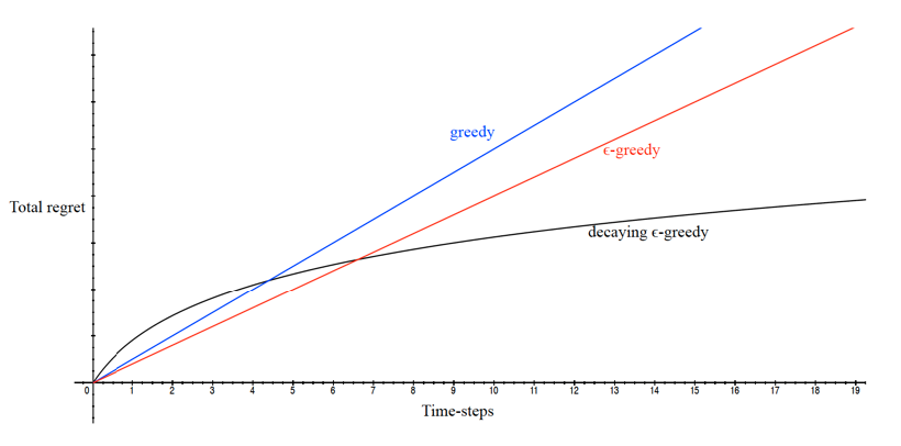
so that we would like to look for a way to get sub-linear total regret.
-
if you never explore, your regret will increase lienearly.
-
for epsilon greedy, similar but slightly better
-
sub-linear: We graduating decrease $\epsilon$ over time, having more exploitation over time.
-
decaying needs some decaying schedule. An example would be
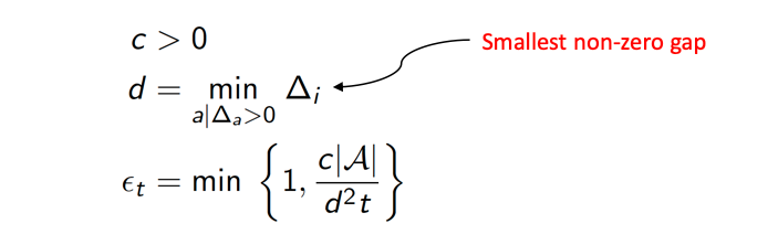
the longer time/steps we have sampled, the less exploration. Also if $d$ is big, meaning currently making big mistakes, we want to reduce exploration
-
But remember that $d$ or $\Delta_a$ is still hard to calculate in practice as we don’t know $V^*$
Upper Confidence Bound
What is the lower bound on Multi-arm bandit in terms of regret? Maybe we can get an algorithm if we know the lower bound?
For instance, let us say we have three actions, and let us model $\hat{Q}(a)$ and we are unsure of our estimate:
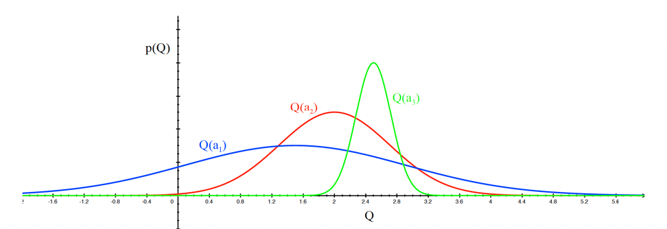
so that uncertainty for each action would be this breadth. The idea is the more uncertain we are about an action, the more important it is to explore it
-
action $a_1$ has the highest breadth/uncertainty, hence pick this first
-
after picking blue, we would be less uncertain as this distribution shifts, and more likely to pick other actions
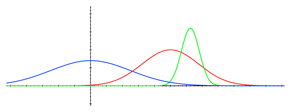
Therefore, we are optimistic in the face of uncertainty by hoping those highly uncertain actions to be potentially very beneficial
An example algorithm to do this is UCB
- $U_t(a)$, if you never tried an action $a$, then this will be very high/high uncertainty
- combine with current estimate $Q$ to combine exploration and exploitation $\hat{Q}_t(a) + \hat{U}_t(a)$
so we select action maximizing UCB
\[a_t = \arg\max_{a \in \mathcal{A}} \hat{Q}_t(a) + \hat{U}_t(a)\]But what is $\hat{U}_t$? It is motivated by the Hoeffding’s Inequality
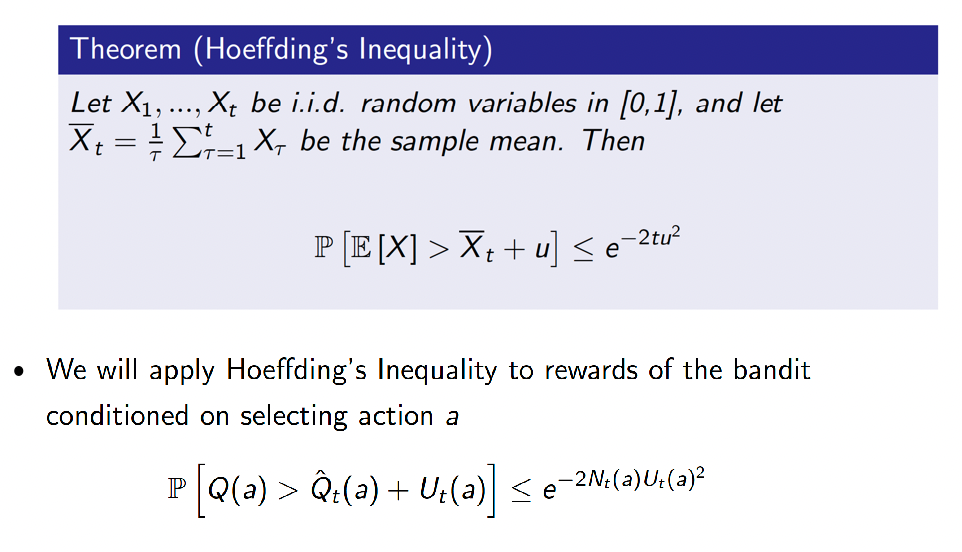
which makes sense in the context of MAB because if we have large uncertainty, then this probability is small. Then we can use this to solve for a form of $U$:
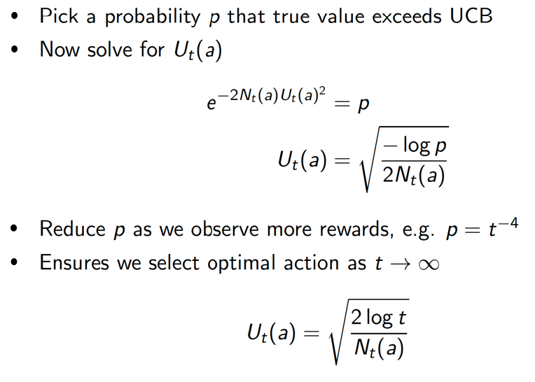
and we knw that this UCB1 achieves sublinear regret on on Multi-arm bandit
Baysesian Bandits
So far made no assumptions about the reward distribution, and this methods basically exploit prior knowledge of rewards by specifying a prior distribution
Have a prior to shape the reward distribution, and use posterior to guide exploration
So that we essentially estimate the posterior based on the (prior probability and the sample) you get:
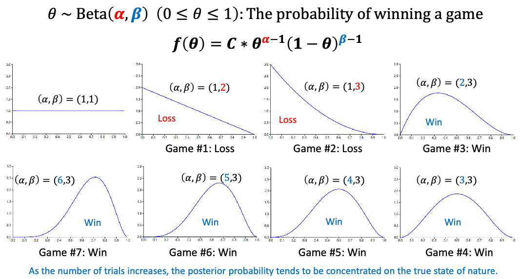
where $\alpha$ is number of times the arm gives you success, $\beta$ number of times if failed. Consider $\theta$ modeling reward we will get form this action. Consider a “success” being a reward $+1$ is given, failure gives $0$ reward
- in the begnning, no idea so $\alpha=\beta=1$ meaning the machine can give you any reward
- if we lost, then the average value drifts to the left
- in the end, you see the average reward is about $0.7$
Once done, now we have a distribution an action. We can repeat this to get a distribution for each action.
Then, how do we decide which action to pick? Since we are doing probability matching, we want take actions respecting those probability. For instance, say you have got three distribution with mean $0.1,0.7,1.0$
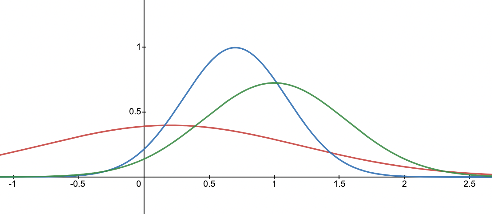
- sample a reward from each curve, say $r_1=0.1,r_2=0.9,r_3=0.7$
- choose an action according to the biggest reward in the sample. Hence action $a_2$
Other more well-fleshed idea is Thompson Sampling:
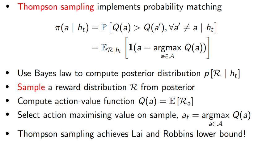
which also achieves the lower bound!
Intuitively, this way you can naturally achieve exploration.
This is also optimistic in the face of uncertainty, because those uncertain actions could have higher probability being $\max$ during sampling
Federated Reinforcement Learning
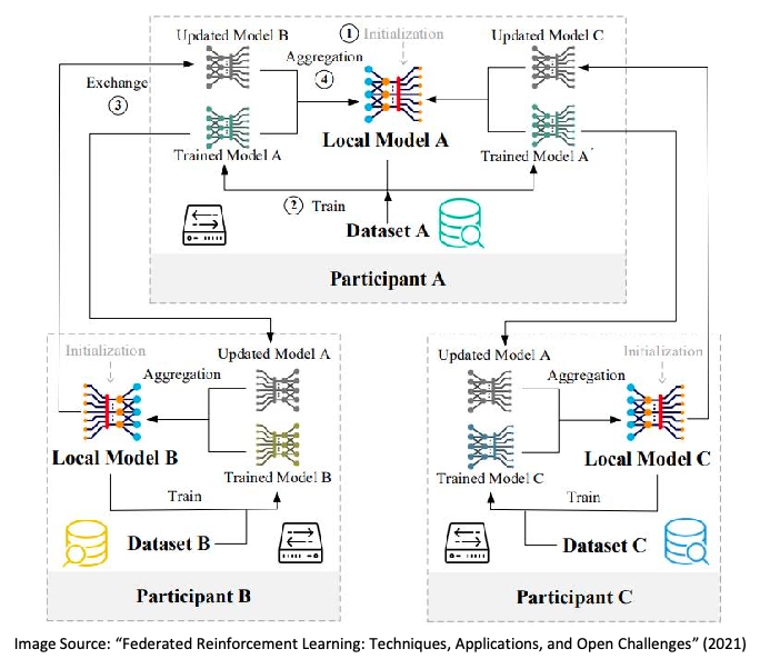
Federated reinforcement learning is a type of reinforcement learning in which multiple agents or agents across multiple devices learn to solve a common problem while maintaining the privacy and autonomy of their local data.
This can be useful in situations where the data that is used to train the learning algorithm is distributed across multiple devices or agents, and where it is not feasible or desirable to centralize the data. (somewhat similar to A3C idea)
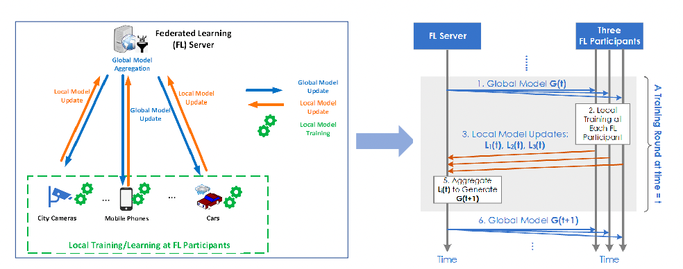
- Advantages: No need for centralized training data collection and centralized, data privacy, edge intelligence, learning quality
- Disadvantages: New threats and attacks to distributed participants (e.g., backdoor attack), communications overhead, varying data quality, selection of FL participant
- to some extent this is similar to A3C
Another approach is learning on the edge:
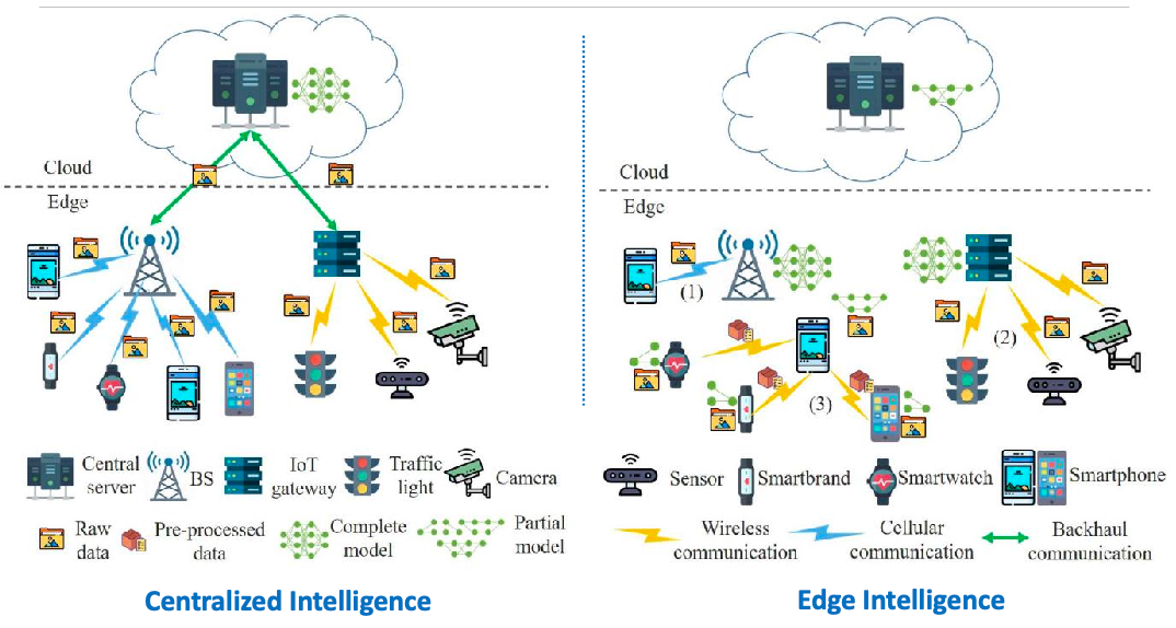
Or you could also have a fully distributed workflow
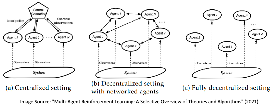
Multi-Agent Reinforcement Learning
Categories in MARL:
- agents are cooperative
- agents are competitive
- hybrid, intra-group cooperation but inter-group competitive
Architectures can look like:
An example success if DeepNash, where the there is incomplete information in the game as well
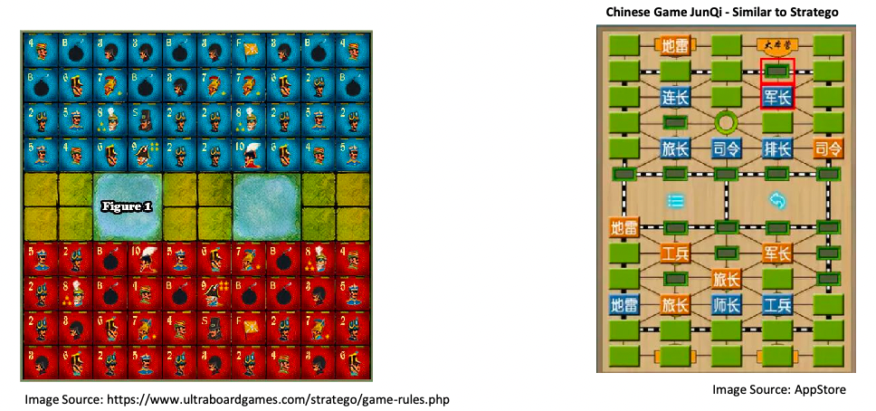
From the paper abstract:
- We introduce DeepNash, an autonomous agent that plays the imperfect information game Stratego at a human expert level.
- Stratego requires long- term strategic thinking as in chess, but it also requires dealing with imperfect information as in poker.
- The technique underpinning DeepNash uses a game-theoretic, model-free deep reinforcement learning method, without search, that learns to master Stratego through self-play from scratch.
RL Part 2 Review
- VFA: estimate $Q \gets \hat{Q}$
- linear approach doing $\hat{Q}=x(s,a)W$
- define loss function using MSE
- gradient has the form $\mathbb{E}[2(\cdot ) \nabla x]$
- if using Q-learning, then the omitted part will be $r+\max_a Q(s’,a’)-Q(s,a)$, etc
- Policy Gradient: score function that the gradient of the loss for improving policy is $Q\cdot\nabla \ln \pi / \mu$
- probably a question on calculating this
- Planning and Learning: planning and learning loop, MCTS
- DRL: differences between DPG and PG, the latter being stochastic policy. More efficient since the action space don’t need to integrated over
- This chapter: trade off between exploration and exploitation, and different methods