PHYS3008 EM n Optics
Recap
Electrostatics
charges stationary $\rho(\vec{r})$ independent of time
| Condition/Name | Equation | Comments |
|---|---|---|
| Basic facts about electric field | $\oint \vec{E}\cdot d\vec{a} = \frac{Q_{enc}}{\epsilon_0}$ | Useful when there is symmetry, so that $\oint \vec{E}\cdot d\vec{a}$ is easy to figure out |
| $V(\vec{r}) = - \int_O^r \vec{E}\cdot d\vec{l}$ | Useful when you already know $\vec{ E}$ | |
| Careful for regions when $\vec{E}$ is not continuous. Then you may need to split your integral. | ||
| $\vec{\nabla}\times \vec{E}=\vec{0}$ | Conservation of field/charge. Proven from showing that $\oint \vec{E}\cdot d\vec{l}=\int \vec{\nabla}\times \vec{E}\cdot d\vec{S}=0$ for a single point charge, then superposition. | |
| A common approach to prove starting from a single point charge, then just use superposition | ||
| $\oint \vec{E}\cdot d \vec{l} = 0$ | from the above. | |
| $\vec{E}=-\vec{\nabla}V$ | Useful for finding out $\vec{E}$, since $V$ is easier to compute | |
| $\nabla^2 V = \rho / \epsilon_0$ | Poisson’s equation. Useful to solve when inside vacuum region such that $\rho = 0$ globally in that region. | |
| In side vacuum, $\nabla^2 V = 0$ is the Laplace Equation | ||
| Over all space | $W=\frac{\epsilon}{2}\int \vert \vec{E}\vert ^2d^3r’$ | Easier to compute, often used. |
| Perfect Conductor | $\vec{E}{meat}=0$, $\rho{meat}=0$ | Charges free to move, will redistribute until $\vec{E}_{meat}=0$. Hence all charges are on the surface |
| $V_{surf}=V_0$, $\vec{E}_{surf}={E}^\perp \hat{n}$ | $V(b)-V(a)=-\int_a^b \vec{E}\cdot d\vec{l}=0$ if on the surface, since $\vec{E}=0$ inside | |
| $V_{meat}=V_0$ as well since there is no field | ||
| Those conditions are often used as constraints in a problem | ||
| Capacitance | $C \equiv \frac{Q}{\Delta V}$ | $Q=+Q$ of the two conductors, is the charge stored |
| $\Delta V =- \int_a^b \vec{E}\cdot d\vec{l}$ commonly used | $\Delta V$ is the potential difference across the two conductor = how much $\Delta V$ needed to store $Q$ | |
| Should be purely geometric, in unit $\epsilon \cdot \text{Length}$ | ||
| Energy Stored in Conductor | $W=\frac{1}{2}\frac{Q^2}{C}=\frac{1}{2}CV^2$ | Think of it being same as energy needed to charge up conductor = work done to move all the charges over |
| Proven because $dW = \Delta V(q)dq$ to move a charge $dq$ over, and then since $C=\frac{q}{\Delta V(q)}$ is geometric, perform $W=\int dW$ | ||
| Summary | 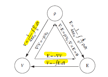 |
Magnetostatics
when you have a steady current, but as it is current, changes are moving $\implies$ magnetic field
| Condition/Name | Equation | Comments |
|---|---|---|
| Biot-Savart Law Generic | $\vec{B}(\vec{r}) = \int \frac{\mu_0}{4\pi} \frac{\vec{J}(\vec{r}’)\times(\vec{r}-\vec{r’})}{\vert \vec{r}-\vec{r’}\vert ^3}\,d^3r’$ | True if $J$ is independent of time, i.e. steady |
| $\vec{E}(\vec{r}) = \int \frac{1}{4\pi \epsilon_0} \frac{\vec{\rho}(\vec{r}’)\cdot(\vec{r}-\vec{r’})}{\vert \vec{r}-\vec{r’}\vert ^3}\,d^3r’$ | parallel to the $\vec{E}$ field, basically $J \to \rho$ | |
| $\mu_0 = 1/(\epsilon_0 c^2)$ | ||
| Biot-Savart if Steady current | $\vec{B}(\vec{r}) = \frac{\mu_0 I}{4\pi} \int \frac{d\vec{l}(\vec{r}’)\times(\vec{r}-\vec{r}’)}{\vert \vec{r}-\vec{r}’\vert ^3}$ | basically we have here $\vec{J} = \vec{I}\delta^2(\vec{r}-\vec{r}’)$ and that $\vec{I}dl = Id\vec{l}$ |
| works if constant current so $\vec{I}dl = Id\vec{l}$ holds | ||
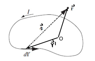 |
Integrates $dl’$ only over where $\vec{r}’ \neq 0$ | |
| Magnetric Field of a Straight line wire | $\vec{B} = \frac{\mu_0 I}{2\pi r} \hat{e}_\phi$ | Found either using Biot-Savart for current, or using the symmetry hence $\oint \vec{B}\cdot d\vec{l} = \mu_0 I_{enc}$ |
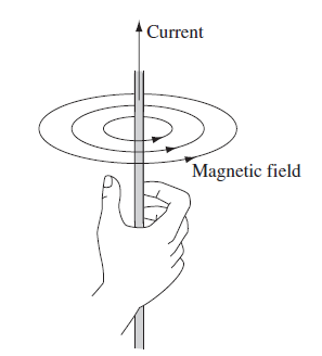 |
Graphically it circulates the current | |
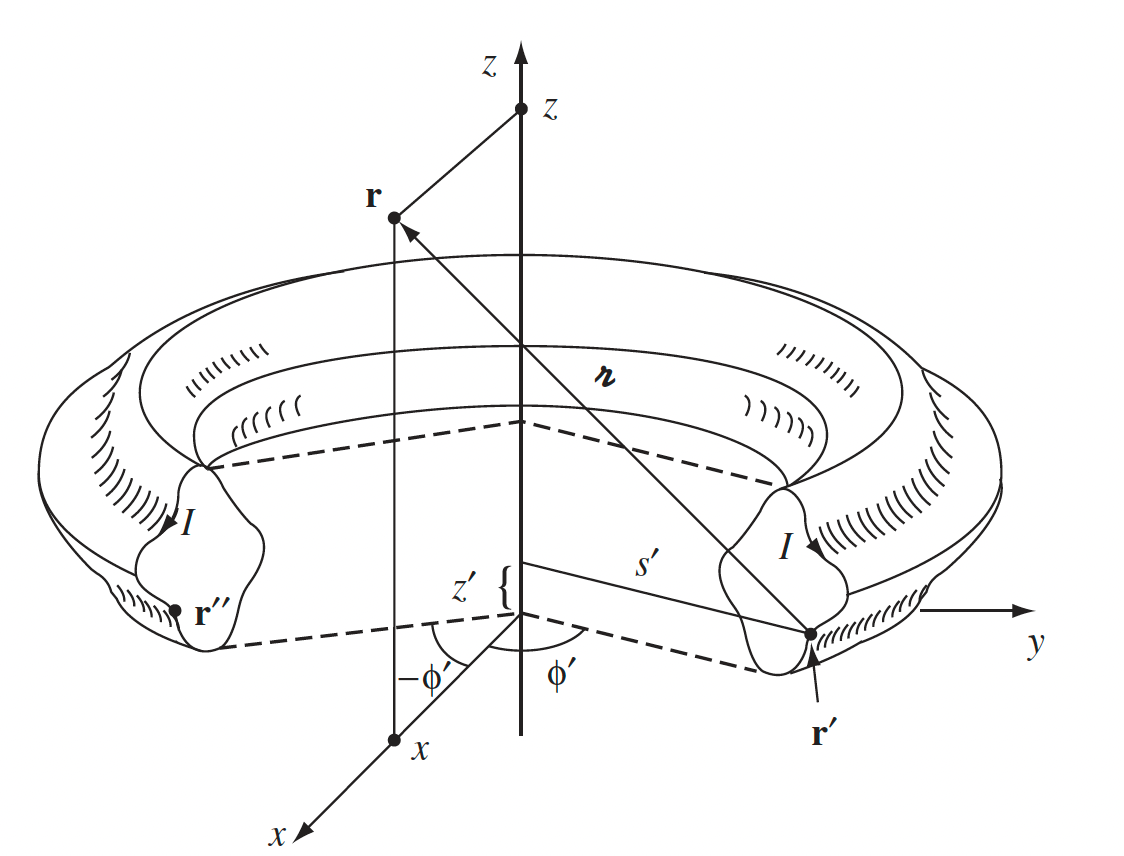
| Field of a Toroid | $B = \frac{\mu N I}{2 \pi s}$ | and $0$ outside. $s$ is basically the radial distance |
 |
||
| Divregence of B | $\vec{\nabla}_{\vec{r}} \cdot \vec{B}(\vec{r})=0$ | for E field we had $\vec{\nabla}\cdot \vec{E}= \rho/\epsilon_0$ |
| $\oint \vec{B}\cdot d\vec{S}=0$ | for E field we had Gaussian surface $\oint \vec{E}\cdot d\vec{S}=Q_{enc}/\epsilon_0$! | |
| derived using $\int \vec{\nabla}\cdot\vec{B} d\tau = \oint \vec{B}\cdot d\vec{S}$ | ||
| not very useful for B field calculation | ||
| Curl of B | $\vec{\nabla}_{\vec{r}} \times \vec{B}(\vec{r})=\mu_0 \vec{J}(\vec{r})$ | for E field we had this is 0 |
| $\oint \vec{B}\cdot d\vec{l}=\mu_0 I_{enc}$ | very useful for B field calculation if we have symmetry in $J$ or $I$ setup! | |
| called Ampere Loops | ||
| derived using $\int \vec{\nabla}\times \vec{B}\cdot d\vec{S} = \oint \vec{B}\cdot d\vec{l}$ | ||
| Field of Solenoid with $n$ turns per unit legnth | $\vec{B} = \mu_0 n I \hat{e}_z$ | if inside the solenoid |
| $\vec{B}=0$ | if outside | |
 |
Essentially solved by drawing Amphere loops | |
| Magnetic Vector Potential | $\vec{\nabla}\times \vec{A} = \vec{B}$ | so that $\vec{A}$ is easier to compute |
| from $\vec{E}= - \vec{\nabla}V$ for $V$ is easier to compute | ||
| Gauges for $\vec{A}$ due to above definition | $\nabla(\nabla \cdot \vec{A})-\nabla^2\vec{A} = \mu_0 \vec{J}$ | if $\vec{\nabla}\times \vec{A} = \vec{B}$, and we know $\nabla \times \vec{B} = \mu_0 \vec{J}$ |
| if $\nabla \cdot \vec{A} = 0$ | Colomb’s Gauge, used by this course | |
| $\vec{A}’ = \vec{A}+ \nabla\lambda$ results in the same $B$ field | therefore we can always force $\nabla \cdot \vec{A} = 0$ by choosing $\lambda$ | |
| Magnetic Vector Potential Definition | $\vec{A} = \frac{\mu_0}{4\pi}\int \frac{\vec{J}(\vec{r}’)}{\vert \vec{r}-\vec{r}’\vert }d^3r’$ | derived from the above with $\nabla^2 \vec{A}=-\mu_0 \vec{J}$, so that each compontent $A_x,A_y,A_z$ essentially is an analog version of $\nabla^2 V = - \rho / \epsilon_0$ and we know the solution $V$ from using $\rho$ |
| this means that $\vec{A}$ is usually in the same direction as current! | ||
| Technically $\vec{A} = \frac{\mu_0}{4\pi}\int \frac{\vec{J}(\vec{r}’)}{\vert \vec{r}-\vec{r}’\vert }d^3r’ + \vec{A}(0)$ | for $\vec{A}(0)$ is a reference point | |
| usually use $\vec{A}(\infty)=0$ |
Polarization and Magnetization
Basically consider $E$ and $B$ Field inside Matter themselves (e.g. after providing an external $\vec{E}{ext}$ or $\vec{B}{ext}$)
first, we show $E$ fields in matter, i.e. polarization $\vec{P}$, and we are only interested in what field this material will produce, and do not discuss how we get there.
| Condition/Name | Equation | Comments |
|---|---|---|
| Electric Dipole | when a piece of diaelectric material is placed under $\vec{E}_{ext}$, those little dipoles align themselves and form $\vec{P}$ | |
 |
||
| Polarization | $\vec{P}\equiv$dipole moment per unit volume | when a piece of dielectric material is placed under $\vec{E}_{ext}$, those little dipoles align themselves and form $\vec{P}$ |
| Potential due to Polarization $\vec{P}$ | $V(\vec{r}) = \frac{1}{4\pi \epsilon}\frac{\vec{p}]\cdot\hat{r}}{r^2} + O(\frac{1}{r^3})$ | multi-pole expansion of electric potential |
| $V(\vec{r}) = \frac{1}{4\pi \epsilon_0} \oint_\Omega \frac{\sigma_b}{\vert \vert \vec{r} - \vec{r}’\vert \vert }dA’+ \frac{1}{4\pi \epsilon_0} \int_V \frac{\rho_b}{\vert \vert \vec{r} - \vec{r}’\vert \vert }dV’$ | derived from $V(\vec{r})$ above but only consisting of dipole terms | |
| $V(\vec{r})=V(\text{from$\sigma_b, \rho_b$})$ | i.e. you can treat the dielectric as having $\sigma_b$ on the surface and $\rho_b$ inside. | |
| if $\rho_b = 0$, $V(\text{from$\sigma_b,\rho_b$})$ can be solved using Laplacian $\nabla^2 V = 0$ with boundary of $\sigma_b$ | ||
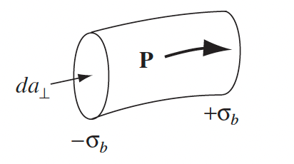
| $\sigma_b \equiv \vec{P}\cdot \hat{n}$ | $\hat{n}$ points from the surface having dielectric to vaccum/non-dielectric place | |
| $\rho_b\equiv - \nabla \cdot \vec{P}$ | ||
| Interpretation of Bound Charge due to $\vec{P}$ | $\sigma_b \equiv \vec{P}\cdot \hat{n}$ | $\sigma_b$ comes from lining up dipoles so that only ends matter |
 |
||
| $\rho_b\equiv - \nabla \cdot \vec{P}$ | $\rho_b$ considers if dipole in between is not cancelled out, then the flux of polarization would relate to charge: $-\oint \vec{P}\cdot d\vec{A} =\int_V \rho_b \,d^3r’$ | |
| Displacement Field | $\nabla \cdot \vec{E}_{total} = (\rho_f+\rho_b) / \epsilon_0$ | since now the polarization also produces field, we want to know a “general” equation for $\vec{E}$ field |
| $\nabla \cdot (\epsilon \vec{E}_{total}+\vec{P}) = \rho_f$ | use $\rho_b\equiv - \nabla \cdot \vec{P}$ | |
| $\vec{D}\equiv \epsilon \vec{E}_{total}+\vec{P}$ | ||
| Gauss Law for Electric Displacement Field | $\nabla \cdot \vec{D} = \rho_f$ | derived from above |
| $\oint \vec{D}\cdot d\vec{A} = Q_{free_{enc}}$ | integral form | |
| if have symmetry can use Gaussian surfaces | ||
| used for proving boundary conditions for $\vec{D}$ | ||
| $\vec{\nabla} \times \vec{D} = \vec{\nabla} \times \vec{P}$ | ||
| $\oint \vec{D}\cdot d\vec{r}=\oint \vec{P}\cdot d\vec{r}$ | Stokes’ Theorem, derived from above | |
| used for proving boundary conditions for $\vec{D}$ | ||
| the above is true for any dielectric | ||
| $\vec{D}$ and $\vec{E}$ relation | $\vec{\nabla}\cdot \vec{E}{tot} = \rho{tot} / \epsilon_0 \to \vec{E}{tot} = \frac{1}{4\pi \epsilon_0} \int \frac{\rho{tot}}{\symscr{r}} \hat{\symscr{r}}\,d^3r’$ | because $\vec{\nabla}\times \vec{E}_{tot} = 0$ |
| $\vec{\nabla}\cdot \vec{D}= \rho_{free} \not\to \vec{D} = \frac{1}{4\pi } \int \frac{\rho_{free}}{\symscr{r}} \hat{\symscr{r}}\,d^3r’$ | because $\vec{\nabla} \times \vec{D} \neq 0$ often, hence $\vec{D}$ might not have a potential | |
| Linear Dielectric | $\vec{P} = \epsilon_0 \chi_e \vec{E}_{tot}$ | $\chi_e$ is electric susceptibility, $\epsilon_0$ is permittivity of free space |
| if $\vec{E}{applied}$ is given, we are stuck because it will produce $\vec{P}$, which produces $\vec{E}{resp}$ hence affects $\vec{E}_{tot}$, which relates to $\vec{P}$… | ||
| $\vec{D} = \epsilon_0(1+\chi_e)\vec{E}{tot}\equiv \epsilon \vec{E}{tot}$ | $\epsilon$ is permittivity of material | |
| can use this to break from the loop if we can find $\vec{D}$ from Gaussian surface | ||
| $\epsilon_r \equiv \epsilon / \epsilon_0 = 1+\chi_e$ | relative permittivity, $\chi_e=0$ in free space. | |
| also called dielectric constant | ||
| $\vec{\nabla}\times \vec{D} = \vec{\nabla} \times (\epsilon \vec{E}_{tot}) \neq 0$ | because $\epsilon$ could vary in different position | |
| Space filled with homogenous Linear Dielectric $\chi_e$ | $\vec{\nabla} \times \vec{D} = 0$, $\vec{\nabla} \cdot \vec{D}= \rho_{free}$ | inside the homogenous linear dielectric, $\epsilon$ is constant |
| $\vec{D} = \epsilon_0 \vec{E}_{free}$ | $\vec{E}_{free}$ is field produced by free charges | |
| because now $\vec{\nabla}\cdot \vec{D}= \rho_{free} \to \vec{D} = \frac{1}{4\pi } \int \frac{\rho_{free}}{\symscr{r}} \hat{\symscr{r}}\,d^3r’$ holds |
Application of Bound Charges
Consider a slab of dielectric with thickness $d$ carrying polarization $\vec{P} = k[1+(x/d)]\hat{x}$ :
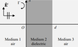
we do not care yet what external field is needed to produce this polarization. We want to know the electric field produced by this given polarization.
First, we can find the bound charges to be:
\[\sigma_b = \vec{P}\cdot \hat{n} = \begin{cases} 2k, & x =d\\ -k, & x=0 \end{cases}\\ \rho_b = -\nabla \cdot \vec{P} = -\frac{k}{d},\quad 0<x<d\]Then, we can treat this as real charges to compute $V(\vec{r})$ due to the correctness of:
\[V(\vec{r}) = \frac{1}{4\pi \epsilon_0} \oint_\Omega \frac{\sigma_b}{||\vec{r} - \vec{r}'||}dA'+ \frac{1}{4\pi \epsilon_0} \int_V \frac{\rho_b}{||\vec{r} - \vec{r}'||}dV'\]Now, since we know the charge distribution, we can exploit the symmetry and save doing the above extra integrals:
-
drawing Gaussian surfaces inside/outside the slab gives:
\[\vec{E}_< = \vec{E}_>\\ (\vec{E}_{inside}-\vec{E}_{<})\cdot \hat{x} = \frac{k}{\epsilon_0}\left(1+\frac{x}{d}\right)\] -
but notice that the net charge is zero, hence:
\[\vec{E}_< = \vec{E}_> = \vec{0}\\ \vec{E}_{inside} = -\frac{k}{\epsilon_0}\left( 1+ \frac{x}{d} \right)\]
the result is consistent if you compute from $\vec{D}$ and use $\vec{D}=\epsilon \vec{E}_{tot}$.
Treating $\sigma_b,\rho_b$ as real charges:
Basically it works due to the proof that
\[V(\vec{r}) = \frac{1}{4\pi \epsilon_0} \oint_\Omega \frac{\sigma_b}{||\vec{r} - \vec{r}'||}dA'+ \frac{1}{4\pi \epsilon_0} \int_V \frac{\rho_b}{||\vec{r} - \vec{r}'||}dV'\]Then, consider finding $V(r)$ for $r < a$ in the setup below:
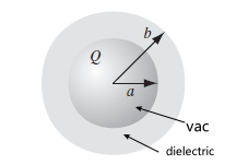
where $Q$ is a point charge sitting at origin. Then, we first can easily figure out $\vec{D}$ by:
\[\int \vec{D}\cdot d\vec{S} = Q_{free_{enc}} = Q,\quad \text{true for all space}\]hence we get:
\[\vec{D} = \frac{Q}{4 \pi r^2}\hat{r}\to \vec{E}_{tot} = \frac{Q}{4\pi \epsilon r^2}\hat{r}\]for $\epsilon$ actually changes in regions, so that:
- $\epsilon=\epsilon_0$ in vacuum hence $r < a$ or $r > b$
- $\epsilon =\epsilon_r \epsilon_0$ inside dielectric
Though we can proceed easily to find $V(\vec{r})$ now, but we can show that we obtain the same result if we treating $\sigma_b,\rho_b$ as real charges:
-
to find $\sigma_b, \rho_b$, first we need to find $\vec{P}$:
\[\vec{P} = \epsilon_0 \chi_e \vec{E}_{tot} = \frac{\epsilon_0 \chi_e Q}{4\pi \epsilon r^2}\hat{r}\] -
then find $\sigma_b, \rho_b$:
\[\sigma_b =\vec{P}\cdot \hat{n} = \begin{cases} -\frac{\epsilon_0 \chi_e Q}{4\pi \epsilon a^2} , & x =a\\ \frac{\epsilon_0 \chi_e Q}{4\pi \epsilon b^2} , & x =b \end{cases}\\ \rho_b = -\nabla \cdot \vec{P} =0,\quad a<x<b\]
Then we can consider $\vec{E}_{tot}$ from those charges while using symmetry:
\[\begin{cases} \vec{E}_{<} = \frac{Q}{4 \pi \epsilon_0 r^2} \hat{r}, & r < a\\ \vec{E}_{inside} = \frac{Q+Q_b(a)}{4 \pi \epsilon_0 r^2} \hat{r}= \frac{Q}{4 \pi \epsilon_0(1+\chi_e) r^2} \hat{r}, & a<r <b\\ \vec{E}_{>} = \frac{Q}{4 \pi \epsilon_0 r^2} \hat{r}, & r > b \end{cases}\]using $\oint \vec{E}\cdot d\vec{A} = Q_{enc}/\epsilon_0$, where:
- $Q_b(a)$ is the bound charges at $r=a$, which is $4 \pi a^2 \sigma_b(a)$.
- this is consistent with $\vec{E}_{tot} = \frac{Q}{4\pi \epsilon r^2}\hat{r}$.
Finally, finding $V(\vec{r})$ for $r < a$ is just doing the integral:
\[V(\vec{r}) = -\int_\infty^r \vec{E}\cdot d\vec{r} = -\int_\infty^b \vec{E}_<\cdot d\vec{r}-\int_b^a \vec{E}_{inside}\cdot d\vec{r}-\int_a^r \vec{E}_>\cdot d\vec{r}\]for $d\vec{r}=dr \hat{r}+ rd\theta \hat{\theta}$.
Magnetization in matter is essentially the same as polarization, but here due to tiny current loops:
| Condition/Name | Equation | Comments |
|---|---|---|
| Magnetic Dipoles | $\vec{m} = I \int d\vec{A}$ | magnetic dipole of a small current loop |
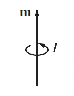 |
derived from multi-pole expansion of $\vec{A}$, and since the mono-pole term is zero, the first order term is dipole. | |
| if you look into any material, electron orbit themselves/spinning = constitute tiny current loops = dipole. However, most material has “no magnetization” because those dipoles are randomly oriented | ||
| But when an external field $\vec{B}_{\mathrm{ext}}$ is supplied, you get some net orientations = net magnetization $\vec{M}$ | ||
| Magnetic Moment $\vec{M}(\vec{r})$ | $\vec{M}(\vec{r})\approx \sum \vec{m}$ | think of $\vec{M}$ as specifying a collection of tiny dipoles $\vec{m}$ |
| $\vec{M}\equiv$ dipole moment per unit volume | for continuous case | |
| $\vec{A}$ from $\vec{M}$ | $\vec{A}=\frac{\mu_0}{4\pi} \sum_{i} \frac{\vec{m}\times \hat{r}}{\vert \vec{r}-\vec{r}_i’\vert }$ | discrete case |
| $\vec{A}=\frac{\mu_0}{4\pi} \int \frac{\vec{M}\times \hat{r}}{\vert \vec{r}-\vec{r}’\vert }d^3r’$ | continuous case | |
| note that $\hat{r}=\vec{r}/\vert \vec{r}\vert$ | ||
| $\vec{A}_{dip} = \frac{\mu_0}{4\pi} \frac{\vec{m}\times \hat{r}}{\vert \vec{r}-\vec{r}’\vert }$ | derived because we know the field of a single dipole | |
| Most generic form of finding $\vec{B}$ from given $\vec{M}$ | ||
| $\vec{A}$ from $\vec{M}$ using bound currents | $\vec{A}=\frac{\mu_0}{4\pi} \int_{all} \frac{\vec{J}_{b}}{\vert \vec{r}-\vec{r}’\vert }d^3r’+\frac{\mu_0}{4\pi}\oint \frac{\vec{K}_b}{\vert \vec{r} - \vec{r}’\vert }dA’$ | mathematically same as above, derived from the continuous case |
| $\vec{J}b \equiv \nabla \times \vec{M},\quad \vec{K}{b} \equiv \vec{M}\times \hat{n}$ | for $\hat{n}$ points from the magnetized material to vacuum | |
| Physical Interpretation of Bound Charges | $\vec{K}_b = \vec{M}\times \hat{n}$ | surface current = current on the surface of material = treat as normal current and compute $\vec{B}$ |
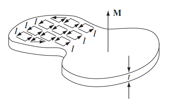 |
imagine uniform magnetized material = uniform tiny current loops | |
| Hence inner loops cancel, we only have net outer current | ||
| $\vec{J}_b = \nabla \times \vec{M}$ | If non-uniform magnetized material, then net $\vec{J}_b$ comes from difference in current loops | |
| Auxiliary Field $\vec{H}$ | same motivation as $\vec{D}$, now in magnetism we have both contributions from $J_f$ and $J_b$ | |
| $\vec{H}=\frac{1}{\mu_0}\vec{B}-\vec{M}$ | more useful than $\vec{B}$ when we have magnetized material | |
| $\vec{H}$ often in the same direction as $\vec{B}$ and $\vec{M}$ | ||
| The magnetic parallel of $\vec{E}$ field. ($\vec{B}$ would be a parallel to $\vec{D}$ instead) | ||
| $\nabla \times \vec{B} = \mu_0 \vec{J}{total} = \mu_0 (\vec{J}_b + \vec{J}{free})$ | derivation from Ampere’s Law, then use $\vec{J}_b = \nabla \times \vec{M}$ | |
| true in general | ||
| Differential and Integral form of $\vec{H}$ | $\nabla \times \vec{H} = \vec{J}_{free}$ | follows from the above |
| $\oint \vec{H}\cdot d\vec{l} =\int \vec{J}{free} \cdot d\vec{A}=I{free_{enc}}$ | very useful when we have symmetry | |
| Linear Material | $\vec{M} \equiv \chi_m \vec{H}$ | $\vec{J}{free} \to \vec{B}{free}\to \vec{M}$ if material is magnetizable |
| $\vec{B}= \mu_0 (1+ \chi_m)\vec{H}=\mu \vec{H}$ | derived from $\vec{H}=\frac{1}{\mu_0}\vec{B}-\vec{M}$ | |
| $\mu = \mu_r \mu_0 \equiv \mu_0(1 + \chi_m)$ |
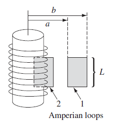
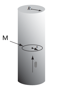
Calculate $\vec{B}$ from Bound Currents
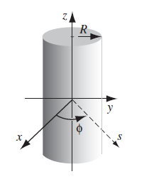
Suppose you are given a material with frozen in magnetization such that $\vec{M}=M\hat{e}_z$ inside the cylinder. The question is what is the magnetic field everywhere.
| Setup | Setup with Bound Currents |
|---|---|
 |
 |
We know we can get $\vec{B}$ either:
- calculate $\vec{A}$ then do $\vec{B}=\nabla \times \vec{A}$. You wil see that we have many ways to find $\vec{A}$
- if finite currents to integrate through, consider treating them as rotating charge = current loops $\vec{A}{dip} = \int d\vec{A}{dip}^{loop}$
- or compute $\vec{A}$ from the bound charges using the generic formula above (a lot of work)
- calculate $\vec{B}$ directly by treating bound currents as currents (faster here)
- calculate using $\vec{H}$, and then convert back with $\vec{H}=\frac{1}{\mu_0}\vec{B}-\vec{M}$ (works, left to you as a mental exercise)
- furthermore, if $\vec{J}_b=0$ and $\nabla \cdot \vec{M}=0$, then can use $\vec{H}=-\nabla W$ and solve laplacian
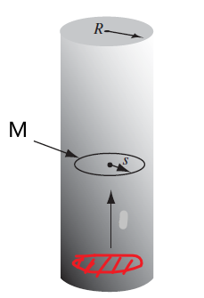
We first compute the bound currents and notice that:
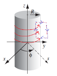
\[\begin{align*} \vec{J}_b &= \nabla \times \vec{M} = \vec{0}\\ \vec{K}_b &= \vec{M}(\vec{r})|_{surf}\times \hat{n} = \begin{cases} 0, & \text{at top/bottom with }\hat{n} = \hat{e}_z\\ M\hat{e}_\phi & \text{at sides with }\hat{n} = \hat{e}_r \end{cases} \end{align*}\]With this we have the graph on the right, for currents going around the cylinder. In this case, we know that $\vec{B}=B_z\hat{e}_z$, which makes the computation straightforward.
Then we can easily compute $\vec{B}$ given this current by drawing ampere loop:
\[\oint \vec{B}\cdot d\vec{l} = \mu_0 I_{enc}\]Knowing that $\vec{B}_{outer}=\vec{0}$ from a solenoid, we have:
\[B_z(r)L - 0 = \mu_0 L K_b = \mu_0LM\]Hence we obtain
\[\vec{B}(\vec{r}) = \begin{cases} \mu_0 M \hat{e}_z, & r < a\\ 0, & r > a \end{cases}\]which makes sense by right hand rule.
Calculate field using $\vec{H}$ from given $\vec{M}$:
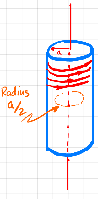
Consider given that $\vec{M} = kr^2 \hat{e}_{\phi}$ inside a cylinder
| Setup | Ampere Loop |
|---|---|
 |
 |
Then we first know that the field $\vec{B},\vec{H}$ would therefore also be in $\hat{e}_{\phi}$ direction (do not confuse $\vec{M}$ with bound currents here). Hence drawing a Ampere loop inside:
\[\oint \vec{H}\cdot d\vec{l} = 2\pi r H_\phi(r)= I_{free_{enc}} = 0\]Hence we easily get $\vec{H}=0$ everywhere. Finally using $\vec{H}=\frac{1}{\mu_0}\vec{B}-\vec{M}$ we get back $\vec{B}$ field by:
\[\vec{B} = \begin{cases} \mu_0 kr^2 \hat{e}_\phi, & r < a\\ 0, & r > a \end{cases}\]since we know $\vec{M}$ as they are given.
- an exercise of this would be to compute using bound currents and arrive at the same solution here.
When to use $\vec{H}$
In general, we can do ampere loops with $\vec{B}$ if we are sure we know all contributions (e.g. from current and from $\vec{M}{induced}$). But consider the case where you have a magnetizable cylinder with some external currents $\vec{J}{free} = I/(\pi R^2)\hat{e}_z$ following through
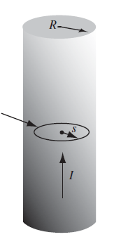
The finding $\vec{B}$ naively using the loop above would give wrong result:
\[2\pi B_\phi(r) = \mu_0 I \pi \left( \frac{r}{R}\right)^2\]but then you have ignored $\vec{M}_{induced}$ which could cause other components in $\vec{B}$. Therefore, the correct way is to consider $\vec{H}$:
\[2\pi H_\phi(r) = I \pi \left( \frac{r}{R}\right)^2\]then using $\vec{H}=\frac{1}{\mu_0}\vec{B}-\vec{M}$ we get $\vec{B}$ (assuming $\vec{M}$ is linear)
Chapter 7 Electrodynamics
| Condition/Name | Equation | Comments |
|---|---|---|
| Ohm’s Law | $\vec{J}=\sigma \vec{E} = nq\vec{v}$ | when you here you have a conductor, this applies |
| $\vec{J}=\sigma \vec{f}=\sigma(\vec{E}+\vec{v}\times \vec{B})$ | how the above comes about = charges move given the force $\gets$ $\vec{B}$ is generally ignored | |
| consistent with perfect conductor $\vec{E}_{meat}=0$, which refers to steady state position | ||
| Mean free path $\lambda$ | $\bar{v} = \frac{1}{2}at = {a \lambda}/{2v_{thermo}}$ | why is current $\propto \vec{E}$ consistent with $\vec{F}=m\vec{a}\propto \vec{E}$? Because electrons zig-zags in material |
| hence what mattered is their average velocity $\propto \vec{E}$ | ||
| Resistance (easy) | $R=\frac{l}{A\sigma}=\rho\frac{l}{A}$ | |
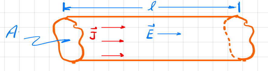 |
derived from $\vec{J}=I/A=\sigma \vec{E}$ in wire, then since $\vec{E}l=V$, you get $I(A/l)=\sigma V$ | |
| EMF | $\varepsilon = \oint {\vec{F}_{source}}/{q}\cdot dl$ | |
 |
fundamentally comes from why current is uniform: there are two forces acting on the electrons: $F_{total}=F_{ext}+ qE$ | |
| then if we consider the net effect over the entire loop $\oint \vec{E}\cdot d\vec{l}=0$ | ||
| an example of $F_{ext}$ could be battery providing chemical power/”force” | ||
| Motional EMF | $\varepsilon = -d\Phi / dt$ | insight from below. Same physics as Lorentz force |
| $\varepsilon = \oint (qvB/q) \ dl=vBl$ | because magnetic force $q\vec{v}\times \vec{B}$ contributes to $F_{total}$, but integral over a loop is non-zero | |
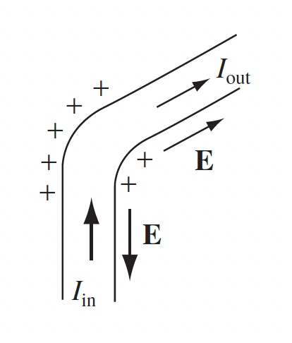
| Induced Electric Field/Faraday’s Law | $\nabla \times \vec{E} = -\partial \vec{B} / dt$ | |
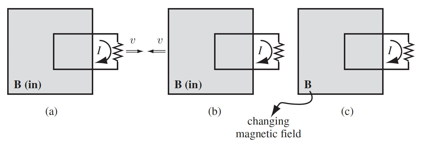 |
all three methods create moving charges = current, but only the first one is due to magnetic force (Lorentz) | |
| In the second and third, charges are static but we know they still moved $\gets$ there is an induced electric field | ||
| $-d\Phi /dt = \oint \vec{E}\cdot d\vec{l}=\varepsilon$ (by definition) | changing magnetic field induce electric field $\vec{E}$ | |
| from this $\varepsilon$ you can find the induced current | ||
| Lenz’ Law | nature abhors change in flux | used to determine the direction of induced current from Faraday’s law |
| Mutual Inductance | $\Phi_1 = M_{12}I_2$ | $M_{12}$ would be the coefficient for the $\vec{B}_{21}$ field produced (from 2 on 1) as a function of $I_2$ |
| $M_{12}=M_{21}$ | purely geometric, independent of current | |
 |
an example would be realizing $\Phi_1$ for the inner loop is just some geometric factor $\times I_2$. (recall that $B=\mu_0 n I$ for solenoid) | |
| Self Inductance | $\Phi = LI$ | because its own current creates magnetic field |
| Inductance | $\Phi_1 = L_1 I_1 +M_{12}I_2$ | but in general we assume $I_2 » I_1$ |
| Back EMF | $\varepsilon_{back} = -L dI/dt$ | derived from $\Phi=LI$ |
| therefore, $L$ is like inertia mass: the higher it is, harder for current to move/start moving | ||
| Energy in circuit with $L$ | $U=(1/2)L I^2$ | derived from $W_q = -\varepsilon_{back}q$ which is the work done needed to push charges one loop when I tuned on the circuit |
| then take $/dt$ on both sides, and integrate get $\int dU = L \int IdI$ | ||
| Energy stored in magnetic field | $U_B = (1/2\mu) \int_{\text{all space}} \vert B\vert ^2 dV$ | derived from the above, and using $LI = \Phi = \int \vec{B}\cdot d\vec{A}$ |
| consistent with the above. Hence can also be used to find $L$. | ||
| Maxwell’s Equation | replacing the below to have $\nabla \times \vec{B}=\mu_0 \vec{J} +\mu_0 \epsilon_0 \frac{\partial \vec{E}}{\partial t}$ | |
 |
realizing this form before is inconsistent if you test $\nabla \cdot (\nabla \times \vec{B})$ in case of electrodynamics, i.e. $d\rho /dt \neq 0$ | |
| now, this means changing $\vec{B}$ will change $\vec{E}$, and also vice versa | ||
| essentially, these equations tells you how charges/currents produce fields. | ||
| Change in polarization $\vec{P}$ cause new current | $\frac{\partial \vec{P}}{dt}=\vec{J}_p$ | |
 |
if $\vec{P}$ increased, then it means we also have changed $\sigma_b$: $dI = \frac{\partial \sigma_b}{dt}dA$ | |
| since $\sigma_b = \vec{P}\cdot \hat{n}$, we get $dI/da = \partial \vec{P}/dt$ | ||
| Current and Charge in material | $\rho_{total} = \rho_{free} + \rho_b = \rho_{free} - \nabla\cdot\vec{P}$ | since we can only control free charge, we want to express field only as a function of free charge |
| $\vec{J}{total} = \vec{J}{free} + \vec{J}b + \vec{J}_p = \vec{J}{free}+\nabla\times \vec{M} + \frac{\partial \vec{P}}{\partial t}$ | then we just plug those in Maxwell’s equation, which holds for $\vec{E}{total}$ and $\vec{B}{total}$ | |
| Maxwell’s Equation in Material | 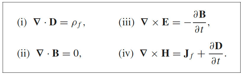 |
why is there a difference? Inside material we need to also consider effect from polarization $\vec{P}$ and magnetization $\vec{M}$ |
| $\vec{D}=\epsilon_0\vec{E}+\vec{P}$ $\vec{H}=\frac{1}{\mu_0}\vec{B}-\vec{M}$ |
||
| compared to the one in vacuum, there is an extra term $\partial D / \partial t\equiv \vec{J}_D$ named to be displacement current | ||
| e.g. inside a conducting material, you will have $\vec{J}_{f}=\sigma\vec{E}$ free charges moving and another $\vec{J}_D=\partial \vec{D}/dt$ if there is a change in field. | ||
| summarizes the fields to include contribution from polarization and magnetization, but as a function of free charges and current | ||
| linear material | $\vec{D}=\epsilon \vec{E}$; $\vec{H} = \frac{1}{\mu}\vec{B}$ | often used to simplify Maxwell’s equations in material to get only E and B |
| if you insert this into Maxwell’s equation in material and use $\mu \to \mu_0, \epsilon\to \epsilon_0$, you get back the equation in vaccum! | ||
| Integral form of Maxwell’s Equations | 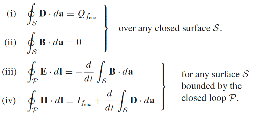 |
can be used to calculate fields |
| also for later chapters, essentially determines the boundary conditions when solving equations | ||
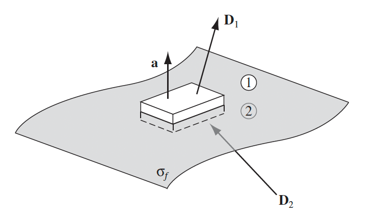
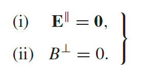
| Boundary Conditions | $D^\perp_1 - D^\perp_2 = \sigma_{free}$ $B^\perp_1 - B^\perp_2 = 0$ |
derived using the geometry below |
 |
||
| $\vec{E}^\parallel_1 - \vec{E}^\parallel_2 = 0$ $\vec{H}^\parallel_1 - \vec{H}^\parallel_2 = \vec{K}_{free}\times \hat{n}$ |
derived using the geometry below. | |
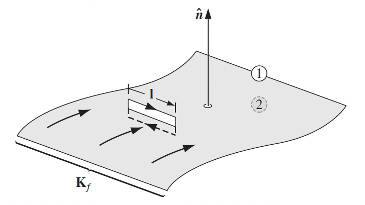 |
$\vec{K}{free}$ comes from the possibility $I{f_{enc}}\neq0$, and $\times \hat{n}$ is due to the direction requirement that $I_{f_{enc}} = \vec{K}_f \cdot (\hat{n}\times \vec{l})=(\vec{K}_f \times \hat{n})\cdot \vec{l}$ | |
| Boundary Conditions for Linear Media | 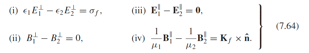 |
simply when $\vec{D}=\epsilon \vec{E}$; $\vec{H} = \frac{1}{\mu}\vec{B}$ |
| used quite often as we almost always have a linear media and this form is only in $\vec{E}$ and $\vec{B}$ |
Connection between electrostatics, magnetostatics, induced field:
| Electrostatics | Magnetostatics | Faraday’s Induced E field |
|---|---|---|
| $\nabla \cdot \vec{E}=0$ | $\nabla \cdot \vec{B}=0$ | $\nabla \cdot \vec{E}=0$ |
| $\nabla \times \vec{E}=0$ | $\nabla \times \vec{B}=\mu_0 \vec{J}$ | $\nabla \times \vec{E} = -\partial \vec{B} / dt$ |
| $\oint \vec{E}\cdot d\vec{l}=0$ | $\oint \vec{B}\cdot d\vec{l}=\mu_{0} I_{enc}$ | $\oint \vec{E}\cdot d\vec{l}=-d\Phi / dt$ |
Transformer and using Inductance.
Consider the task is to find out (a) show that $V_1/V_2 = N_1/N_2$, (b) that $M^2=L_1L_2$, and (c) the differential equation to solve for $I_1(t),I_2(t)$
-
let the magnetic flux for a single turn be $\Phi_0 = \vert \vec{B}\vert A$. Then we get
\[\varepsilon_1 = N_1 \frac{d\Phi_0}{dt},\quad \varepsilon_2 = N_2 \frac{d\Phi_0}{dt}\]then just divide
-
We know that also
\[\Phi_1 = L_1I_1 + M_{12}I_2 = N_1 \Phi_0\\ \Phi_2 = L_2I_2 + M_{21}I_1 = N_2 \Phi_0\]then eliminating $\Phi_0$, and find
\[\frac{L_1}{N_1}I_1 + \frac{M_{12}}{N_1}I_2 = \frac{L_2}{N_2}I_1 + \frac{M_{21}}{N_2}I_1\]but as $M$ is purely geometric, this should hold even if $I_1=0$ and when $I_2=0$. From which you can show that $M_{12}M_{21}=L_1L_2$
-
Let there be an external power giving $V_1\cos(\omega t)$ at $\varepsilon_1$. Then for this to hold, we must have:
\[\varepsilon_1 = -\frac{d\Phi_1}{dt} = -(L_1\dot{I_1} + M_{12}\dot{I}_2) = -V_1 \cos(\omega t)\]so basically ODE with $dI/dt$ but coupled
How do you find inductance $L$?
One trick is to realize that
\[\Phi = LI = \int \vec{B}\cdot d\vec{A}\]then you just need to massage the RHS to have $(\text{something})\cdot I$.
Another trick is to use energy. Since energy stored of the circuit = energy of the fields, e.g. for a solenoid
\[U = \frac{1}{2\mu_0}\int |B|^2 dV = \frac{1}{2}LI^2\]and there are no electric fields as wires are charge neutral.
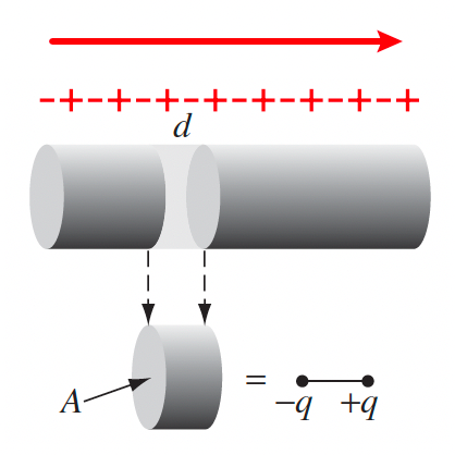
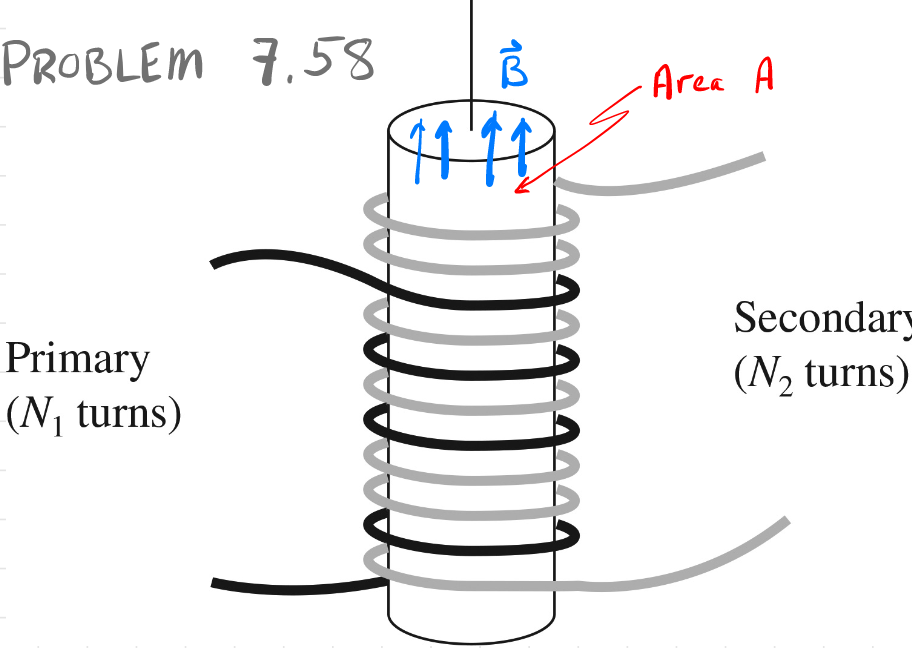
Using Maxwell’s Fix on Ampere’s Law
Consider finding $\int BdA$ given this Amperian loop.
From $\nabla \times \vec{B}=\mu_0 \vec{J} +\mu_0 \epsilon_0 \frac{\partial \vec{E}}{\partial t}$, this means
-
using the circular disk are:
\[\oint \vec{B}\cdot d\vec{l} = \mu_0 I_{enc} = \mu_0 I\] -
if we use the version $\nabla \times \vec{B}=\mu_0 \vec{J}$, then we will get $0$. But:
\[\oint \vec{B}\cdot d\vec{l} = \mu_0 I_{enc} + \mu_0 \epsilon_0 \int_S \frac{\partial \vec{E}}{\partial t}\cdot d\vec{A}\]since there is no $I_{enc}=0$, but the electric field within the gap is changing as $\vec{E}(t)=\sigma(t)/\epsilon_0$:
\[\oint \vec{B}\cdot d\vec{l} = \mu_0 \epsilon_0 \int_S \frac{\partial }{\partial t}\frac{Q(t)}{\epsilon_0 A}\cdot d\vec{A}\]since $dQ/dt=I$, we recover the same expression as 1.
Chapter 8 Conservation Laws
Basically how we get energy and momentum from fields themselves = found that in order for conservation of energy/momentum to work, we need to attach energy and momentum to fields. How do we know things are conserved?
- if energy $U$ is conserved, then $dU/dt=0$
- if momentum $\vec{p}$ is conserved, then $d\vec{p}/dt = 0$
| Condition/Name | Equation | Comments |
|---|---|---|
| Work Energy Theorem in Electrodynamics | $\frac{dW}{dt}=-\frac{\partial}{\partial t}\int_{V}\underbrace{\left[ \frac{1}{2}\epsilon_0 E^2 + \frac{1}{2\mu_0}B^2\right]}{u{EM}}dV - \int_{\partial V}\underbrace{\frac{1}{\mu_0}(\vec{E}\times \vec{B})}_{\vec{S}}\cdot d\vec{a}$ | $dW$ here represent work done by EM field on charges in a volume $V$ |
| fundamentally, think about how to make charges move = $F=q(\vec{E}+\vec{v}\times \vec{B})$, when find $dW/dt$ in terms of fields. | ||
| $u_{EM} = \frac{1}{2}(\epsilon_0 E^2 + \frac{1}{\mu_0}B^2)$ | $u_{EM}$ represent energy stored in the field in $V$ | |
| $\vec{S}$ represent energy per unit area per time = energy flux going out of $V$ since $d\vec{a}$ points out | ||
| $dW = \vec{F}\cdot d\vec{r} =q\vec{E}\cdot{\vec{v}}dt$, then $dW/dt = \int \vec{J}\cdot \vec{E}dV$ for a density of current | derivation | |
| Poynting Vector | $\vec{S}=\frac{1}{\mu_0}\vec{E}\times \vec{B}$ | energy flux, and also the direction of energy flowing |
| $\frac{\partial }{\partial t}\int_V u dV = - \int_{\partial V}{\frac{1}{\mu_0}(\vec{E}\times \vec{B})}\cdot d\vec{a}$ | why? Consider energy is conserved, $dW/dt=0$. Then if LHS decreases, energy is flowing out and $\vec{S}$ is positive if $\vec{S}$ also points out | |
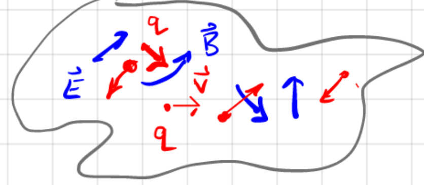
| Need for Maxwell’s Stress Tensor | 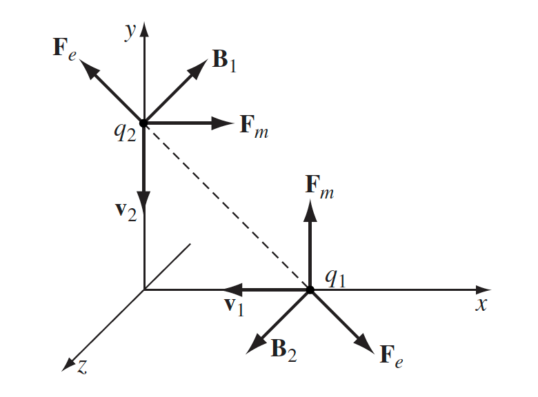 |
Consider the instantaneous fields produced causing those forces. Note that net force $\neq 0$ |
| so momentum is naively not conserved (need to take the fields into account) | ||
| Property of 2D Tensor | 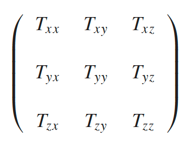 |
one way to visualize $\overleftrightarrow{T}$ |
| $\vec{v}=\begin{bmatrix} v^1\v^2\v^3 \end{bmatrix}=v^i$ | upper index is like a vector component (e.g. $\vec{r} = \begin{bmatrix} x\y\z \end{bmatrix}$) | |
| in our use, upper index often represents coordinate | ||
| $w_i = [w_1, w_2, w_3]$ | lower index usually row vector, or for convenience | |
| in our use, lower index often represents derivative of a coordinate | ||
| Einstein’s Summation Notation | sum over repeated index | |
| $\left( \vec{a} \cdot \overleftrightarrow{T} \right)j = \sum{i}a_i T_{ij}$ = a vector | basically we want the $j$-th vector after this dot product. | |
| in the above visualization, $\vec{a}$ dots into $\overleftrightarrow{T}$ vertically | ||
| $\nabla \cdot \vec{T}^x = \partial_j T^{xj}$ | an example, so $\vec{T}^x$ is the horizontal vector | |
| Maxwell’s Stress Tensor | $T^{ij}=\epsilon_0(E^iE^j - \frac{1}{2}\delta_{ij}E^2)+\frac{1}{\mu_0}(B^iB^j - \frac{1}{2}\delta_{ij}B^2)$ | so $T$ is a 2D tensor (matrix) |
| $\vec{F}_{\text{EM on charges}} = \oint \overleftrightarrow{T}\cdot d\vec{a} - \mu_0 \epsilon_0 \frac{d}{dt}\int_V \vec{S}dV$ | explains why we need the stress tensor | |
| in my practice, even though this is used more often then the differential form, it is better to start your thinking with the differential form | ||
 |
derived from considering force acting on charges due to EM fields, so $\vec{F}=q(\vec{E}+ \vec{v}\times \vec{B})=\int_V (\rho \vec{E}+\vec{J}\times \vec{B})dV$ | |
| $T_{ij}$ represents force acting in the i-th direction on surface oriented in $j$ | ||
| $\vec{F}_{EM}=\oint \overleftrightarrow{T}\cdot d\vec{a}$ | why? if there is no change in fields $d\vec{S}/dt =0$. Then we have this | |
| Momentum of Fields (and conservation) | $\frac{d}{dt}\vec{P}{\text{mechanical}} = - \frac{d}{dt}\int_V \underbrace{\epsilon_0\mu_0\vec{S}}{\vec{g}{EM}}dV + \oint_S \underbrace{\overleftrightarrow{T}}{\text{momentum flux}}\cdot d\vec{a}$ | re-written the same force formula from Maxwell’s Stress Tensor |
| $\frac{d\vec{g}{mech}}{\partial t}=\vec{f}{mech} = \nabla \cdot \overleftrightarrow{T} - \frac{\partial \vec{g}_{EM}}{\partial t}$ | differential form of the above | |
| $\frac{d\vec{g}{mech}^i}{\partial t}=\vec{f}{mech}^i = \partial_jT^{ij} - \frac{\partial \vec{g}_{EM}^i}{\partial t}$ | equation for each component (e.g $i=x,y,z$) | |
| the integral form is used more in practice, but this may be easier to remember and better to start with | ||
| $\frac{d}{dt}\int_V {\epsilon_0\mu_0\vec{S}}dV = \oint_S {\overleftrightarrow{T}}\cdot d\vec{a}$ | how do you interpret this? When there is no change in momentum of charges: | |
| $\vec{g}_{EM} = \mu_0 \epsilon_0 \vec{S}$ | therefore $\overleftrightarrow{T}$ represents momentum flux passing through an area; then naturally $\epsilon_0\mu_0\vec{S}$ is the momentum density inside volume $V$ | |
| Angular momentum of Fields | $\vec{l}{EM} = \vec{r}\times \vec{g}{EM}$ | since it has momentum, the the laws apply |
| $\vec{L}_{EM} = \int_V \vec{l}dV$ | integral form, angular momentum in a volume | |
| questions on this usually involve some charged body starts spinning after there is a change in E or B field (e.g. switched off). This can be explained using the $\vec{l}_{EM}$ in fields |
Example using Poynting Vector
Consider a current flowing down a wire. What is the power in this wire using Poynting vector? Hint: $P=$energy per unit time delivered
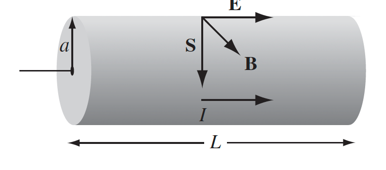
Well, if we know the $\vec{E}$ and $\vec{B}$ field just on the boundary, then
\[\int \vec{S}\cdot d\vec{a} = \text{energy flowing out of }\mathcal{V}\]since since we know $\vec{E}=V/L$, $\vec{B}{surf} = \mu_oI / 2\pi a \,\, \hat{r}\phi$, we get:
\[\vec{S}_{surf} = \frac{VI}{L 2\pi a}\ \text{inwards}\]therefore, energy flows inwards, with power:
\[P = \int Sda = \frac{VI}{L2\pi a}2\pi a L = VI\]A summary of work-energy and momentum equations
Perhaps the differential form is easier to remember:
\[\begin{align*} \text{work-energy conservation}\qquad &\frac{dw_{mech}}{dt} = -\nabla \cdot \vec{S} - \frac{\partial u_{EM}}{dt}\\ \text{momentum conservation}\qquad & \frac{dg_{mech}^x}{\partial t} = \nabla \cdot \overleftrightarrow{T}^x - \frac{\partial g_{em}^x}{dt}\\ & \frac{dg_{mech}^y}{\partial t} = \nabla \cdot \overleftrightarrow{T}^y - \frac{\partial g_{em}^y}{dt}\\ & \frac{dg_{mech}^z}{\partial t} = \nabla \cdot \overleftrightarrow{T}^z - \frac{\partial g_{em}^z}{dt}\\ \text{charge conservation}\qquad &0 = \nabla \cdot \vec{J} + \frac{\partial \rho}{\partial t} \end{align*}\]where note that
- $w_{mech}$ is the work density, i.e. $W_{mech}=\int w_{mech}dV$
- each equation above returns a scalar
- $\overleftrightarrow{T}^x$ would represent the first row of the stress tensor, so that $\nabla \cdot \overleftrightarrow{T}^x = \partial_i T^{xi}$
The take away message here is that field itself has momentum and energy $u_{EM}$ and $g_{EM}$
Example of using Stress Tensor: Calculate the force acting on the upper hemisphere of a uniformly charged sphere:
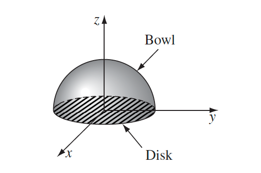
Well, since this is about force, we can consider
\[\vec{F}_{\text{EM on charges}} = \oint \overleftrightarrow{T}\cdot d\vec{a} - \mu_0 \epsilon_0 \frac{d}{dt}\int_V \vec{S}dV\]then this means the closed surface is bowl + disk. First since there is no time dependence, and since we know the net force will be in $\hat{z}$:
\[\vec{F}_{\text{EM on charges}} = \oint \overleftrightarrow{T}\cdot d\vec{a} \quad\to\quad {F}_{z} = \oint \overleftrightarrow{T}^z\cdot d\vec{a} = \oint T^{zi} da_i\]-
force on bowl: the area vector is in spherical coordinate
\[d\vec{a} = R^2 \sin(\theta)d\theta d\phi\ \hat{e}_r\]and using the formula for $T^{ij}$:
\[T^{ij}=\epsilon_0(E^iE^j - \frac{1}{2}\delta_{ij}E^2)+\frac{1}{\mu_0}(B^iB^j - \frac{1}{2}\delta_{ij}B^2)\]since $B=0$, and you know that $\vec{E}$ on the surface is, again in spherical coordinate:
\[\vec{E} = \frac{1}{4\pi \epsilon_0}\frac{Q}{R^2}\ \hat{e}_r,\quad \hat{e}_r=\sin\theta \cos\phi\hat{e}_x + \sin\theta \sin\phi\hat{e}_y + \cos\theta\hat{e}_z\]then compute:
\[T^{zi}da_i = T^{zx}da_x + T^{zy}da_y + T^{zz}da_z\]and do the integral
-
repeat for the disk, using the fact that field inside should go, in polar coordinate:
\[\vec{E}_{disk}=\frac{1}{4\pi \epsilon_0}\frac{Qr}{R^3}\hat{r}\]and
\[d\vec{a} = -r drd\phi \hat{z}\]
but you will see a trick if you start thinking with the local form
\[\vec{f}_{mech} = \nabla \cdot \overleftrightarrow{T} - \frac{\partial \vec{g}_{EM}}{\partial t}\]so that, since outside the sphere there is no charge, $\vec{f}_{mech}=0$. Hence we can consider integrating over a different surface
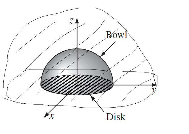
where if we stretch this to be very big, $E\to 0$ at the bowl. Hence we only have the horizontal disk component to integrate
-
force on the outer disk (not touching the charge): in the radial direction
\[\vec{E}_{outer} =\frac{1}{4\pi \epsilon_0}\frac{Q}{r^2}\hat{r}\]with area for $F_z$
\[d\vec{a} = -r drd\phi \hat{z}\]this is much easier then to compute and integrate
\[T^{zi}da_i = T^{zx}da_x + T^{zy}da_y + T^{zz}da_z = T^{zz}da_z\] -
repeat for the inner disk, which is the same as our previous method
Example of Conservation of Angular Momentum (see example 8.4 on textbook) consider a very long solenoid with $n$ turns per length, and inside/outside of it are two cylindrical shell of length $l$ with radius $a,b$, charged with $Q,-Q$ respectively. When $I$ in the solenoid is switched off $I \to 0$, the two cylinders will start to spin. Physically why did this happen? Is angular momentum conserved?
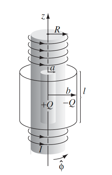
The key mechanism is that there is a change in $B$ field as a result of switching off. Hence:
-
mechanism: there is a change in $B$, hence we get an induced electric field which would act on the charges
\[\nabla \times \vec{E} = -\frac{\partial \vec{B}}{\partial t} \quad \to \quad \oint \vec{E}\cdot d\vec{l} = -\frac{\partial }{\partial t}\int \vec{B}\cdot d\vec{A}\]and since the current is changing, you will get something like:
\[\vec{E}_{s>R} = - \frac{1}{2}\mu_0n\frac{dI}{dt} \frac{R^2}{s}\ \hat{e}_\phi\\ \vec{E}_{s<R} = - \frac{1}{2}\mu_0n\frac{dI}{dt} s\ \hat{e}_\phi\]notice that this field is in the $\phi$ direction, hence the two charged cylinder will feel a torque
\[\vec{N}_b = \vec{r}\times (-Q\vec{E})= \frac{1}{2}\mu_0n QR^2 \frac{dI}{dt} \ \hat{e}_z\]then the angular momentum it has at the end is therefore, using $\vec{N}=d\vec{L}/dt$
\[\vec{L}_{final}-0 = \int_0^t \frac{1}{2}\mu_0n QR^2 \frac{dI}{dt} dt\]then do the same for $\vec{N}_a$ of the smaller cylinder.
-
conservation of angular momentum: you will see from above that $\vec{L}_a + \vec{L}_b$ in the end is not zero. So in the beginning there must be something that is spinning, the field:
\[\vec{l}_{EM} = \vec{r}\times \vec{g}_{EM}\]since the fields in the beginning is:
\[\vec{E} = \frac{Q}{2\pi \epsilon_0 l} \frac{1}{s}, \quad a < s < b \\ \vec{B} = \mu_0 n I\ \hat{e}_z,\quad s<R\]therefore $\vec{g}_{EM}$ is only non-zero inside the solenoid $s < R$. Hence
\[\vec{g}_{EM} = - \frac{\mu_0 n I Q}{2\pi ls} \hat{e}_\phi\]and since we only care about angular momentum in the z-direction:
\[L_{EM}^z = \int_{\text{inside solenoid}} l_{EM}^z\ dV = \int_{\text{inside solenoid}} (\vec{r} \times \vec{g}_{EM})_z \ dV\]you will find this matches up with the angular momentum you found in part 1.
List of good questions:
- Problem 8.2: deal with Poynting vector
- Problem 8.7
- (a),(b) also involves $da_{x},da_y$
- (c) = one way to interpret $T^{ij}$
Chapter 9 EM Waves
Charges and current produce $E$ and $B$ field. The main idea is that in vacuum/material, field themselves need to obey wave equation if we were to also consider the time component of the field = propagate like waves.
-
we will show that in many physical scenarios, solutions have to obey wave equation, e.g. in 1D
\[\frac{\partial^2 y}{\partial x^2} - \frac{1}{v^2}\frac{\partial^2 y}{\partial t^2} = 0\] -
one common solutions is sinusoidal (and you can do Fourier theorem with it to get other functions), and this chapter basically focus on sinusoidal solutions in complex notation, e.g.
\[y(x,t)=\mathrm{RE}[\tilde{A}e^{i(kz-\omega t)} + \tilde{B}e^{i(-kz-\omega t)}]\] -
therefore the physics lies in finding $\tilde{A},\tilde{B},k$ using boundary conditions derived from physical principles (e.g. $B^\perp_1 -B^{\perp}_2=0$)
Plane Waves without $\rho$ and $\vec{J}$
- Plane waves is a simple case of having the amplitudes being a constant in space, e.g. $\tilde{A}$
- without $\rho,\vec{J}$ means we are in vacuum for a good insulator
| Condition/Name | Equation | Comments |
|---|---|---|
| Using Complex Notation | $I(t) = \mathrm{RE}[\tilde{I}_0e^{i\omega t}]$ | if you know the solution of $I(t)$ is in the form of cosine/sine, then using this will almost always make math simpler |
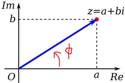
| $\tilde I_0=a+ib = I_0e^{i\phi}$ | so that if $\tilde{I}_0$ is complex, this means we have phase shifts! $\omega t \to \omega t + \phi$ | |
 |
||
| this form is also the nicest if you want to take the real part in the end, which becomes just $I_0 \cos(\omega t + \phi)$ | ||
| Wave “Definition” | 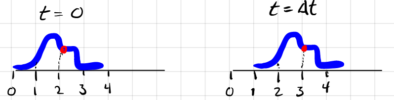 |
a “fixed” shape traveling at some velocity $v$ |
| e.g. $y(x-vt)$, traveling to the right | the fixed shape would be $y(x)$ | |
| e.g. $y(x-vt) = Ae^{-b(x-vt)^2}$ is a valid wave | ||
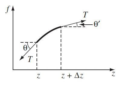
| Wave on String | $\frac{\partial^2 y}{\partial x^2} - \frac{1}{T/\mu}\frac{\partial^2 y}{\partial t^2} = 0$ | so that solution is in the form of $y(x,t)=f(x-vt)+g(x+vt)$ for any function $f,g$ |
| as a result, $v^2 = T/\mu$ is the wave’s traveling speed | ||
| $F_y = T\sin(\theta’)-T\sin(\theta) = (\mu\Delta z) \frac{\partial^2 y}{\partial t^2}$ | derivation, consider force acting on a small section $\Delta z$ of the string, and using $F_y=ma_y$ | |
| $\tan(\theta(x)) = \frac{\partial y}{\partial x}\vert _x$ | then using small angle approx $\sin \approx \tan$, we obtain the wave equation | |
 |
||
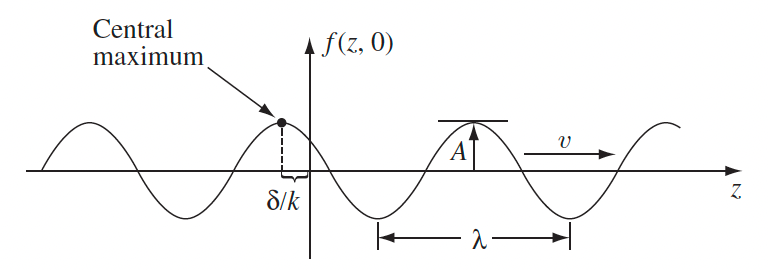
| Sinusoidal Wave | $y(x,t)=A\cos[k(x - vt)+\delta]$ | for waves in physics, sinusoidal form for $f,g$ is considered mostly because (a) it works well with B.C. and (b) any function can be built from them = Fourier theorem |
| $y(x,t)=\mathrm{RE}[\tilde{A}e^{i(kz-\omega t)}]$ | in complex form | |
| $g(x,t)=\mathrm{RE}[\tilde{B}e^{i(-kz-\omega t)}]$ | traveling to the left | |
| hence $k$ indicates direction of propagation | ||
| Important quantities by definition | $\lambda = 2\pi / k$ | by considering $x\to x+(2\pi/k)$ |
| $kv=\omega$, and $\tilde{A}=Ae^{i\delta}$ | wave/phase velocity $v$! | |
 |
||
| start of physics stuff | ||
| B.C. simple reflection and transmission | 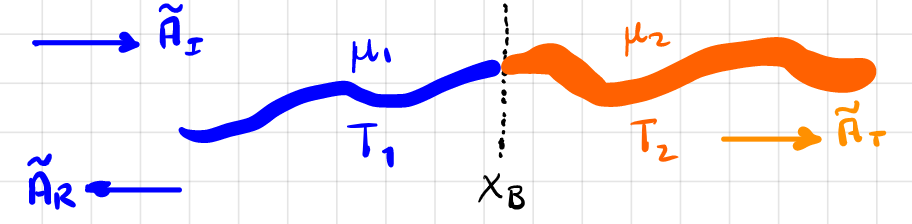 |
string extends to infinity at both ends, and given $\tilde{A}_I$, want to know $\tilde{A}_R,\tilde{A}_T$ |
| assume $\omega$ is the same on both string, hence $\omega=v_1k_1 = v_2k_2$ since velocity has to be different | ||
| $y_<=\tilde{A}_I e^{i(k_1x-\omega t)}+\tilde{A}_R e^{i(-k_1x-\omega t)}$ | waves at $x<x_B$ | |
| $y_> =\tilde{A}_T e^{i(k_2x-\omega t)}$ | waves at $x>x_B$ | |
| $y(0-, t)=y(0+,t)$, $\frac{\partial y}{\partial x}(0-,t)=\frac{\partial y}{\partial x}(0+,t)$ | no B.C. but continuity constraints! | |
| $\tilde{A}_R = \frac{k_1 - k_2}{k_1 + k_2}\tilde{A}_I$ | solve and find | |
| $\tilde{A}_T = \frac{2k_1}{k_1 + k_2}\tilde{A}_I$ | ||
| $\delta_I=\delta_T$, then if $\mu_1 > \mu_2$, $\delta_R = \delta_I$. Otherwise $\delta_R = \delta_I + \pi$ | this has to be given by knowing that $\mu_2 » \mu_1$ gives a standing wave like solution. | |
| In later questions/setups we will also be able to compute the phase shift $\delta$. | ||
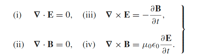
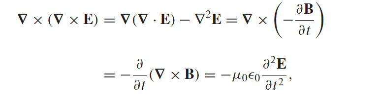
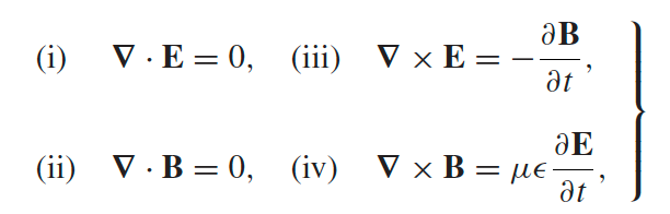
| Wave Equation for EM in vacuum | 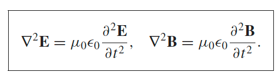 |
derived from Maxwell’s eq assuming $\rho=\vec{J}=0$ |
| so $v^2= 1/\mu_0\epsilon_0=c^2$, so EM waves propagate at speed of light | ||
| notice that this is 3D wave equation. In reality, we will see that when assuming plane waves solution, $E,B$ will be transverse = this reduces to a 1D wave equation | ||
 |
derivation of the above | |
 |
||
| Monochromatic Plane Waves | 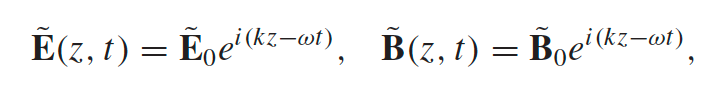 |
assuming that the amplitude vector is constant in all space, i.e. wave looks like a plane |
| $\mathbf{\tilde{E}}_0$ means it is a constant vector but is complex | ||
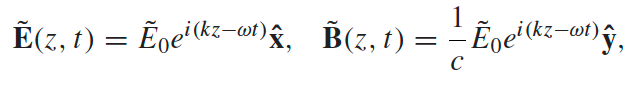 |
almost always the form to start with when solving plane waves question | |
| derived using the “Property of Plane Waves” | ||
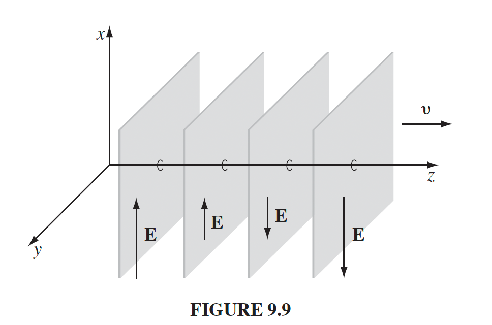 |
up and down is modulated by $e^{i(kz-\omega t)}$ term | |
| Property of Plane Waves | $\tilde{E}_z=\tilde{B}_z = 0$ | because $\nabla \cdot \vec{E}=\nabla \cdot \vec{B}=0$ |
| so EM plane waves are transverse (w.r.t direction of propagation $z$) | ||
| $\mathbf{\tilde{B}}_0 = \frac{1}{c}\hat{z}\times \mathbf{\tilde{E}}_0$ | if $\hat{z}$ is the direction of propagation. So $\mathbf{B}$ is perpendicular to $\mathbf{E}$ and to $\hat{z}$ | |
| derived from $\nabla \times \mathbf = -\frac{\partial \mathbf}{\partial t}$ | ||
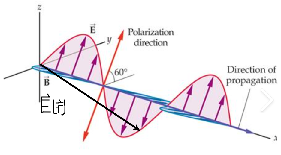
| Wave vector and polarization vector of Plane Waves | 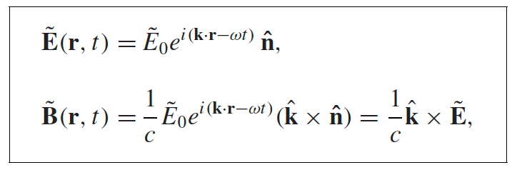 |
$\hat{n}$ is the polarization vector, and $\vec{k}=k\hat{k}$ is the wave/propagation vector |
 |
e.g. $\hat{k}=k\hat{z}$ | |
 |
when you want to know $\vec{E}(\vec{r})$ everywhere in space | |
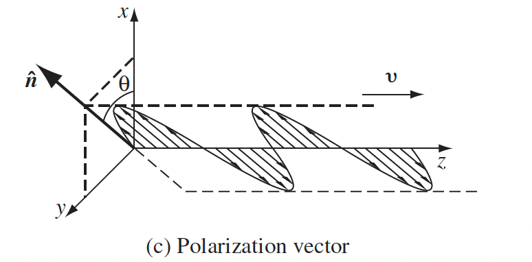
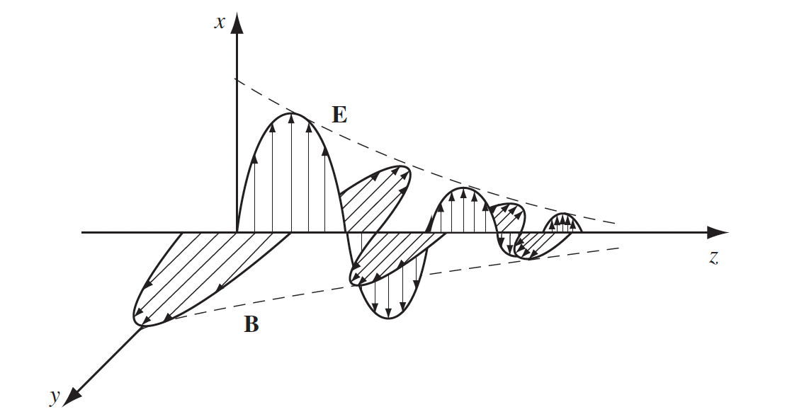
| Visualization of Longitudinal Wave | 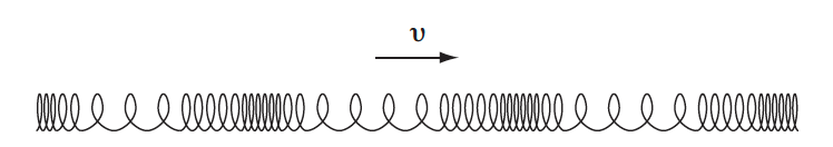 |
this will be useful when considering wave guides = EM waves are not longer purely transverse. But, they are always transverse w.r.t direction of energy propagation $\vec{S}$ |
| Energy in EM Waves | $\lang u_{EM}\rang = \frac{1}{4}(\epsilon_0 \mathbf{\tilde{E}}\mathbf{\tilde{E}}^* + \frac{1}{\mu}\mathbf{\tilde{B}}\mathbf{\tilde{B}}^*)$ | assumes $\mathbf{E}=\mathbf{\tilde{E}}(x,y,z)e^{i(kz-\omega t)}$ and $\mathbf{B}=\mathbf{\tilde{B}}(x,y,z)e^{i(kz-\omega t)}$ |
| time average $\lang u_{EM} \rang = \frac{1}{T}\int_0^T u_{EM}\ dt$ ends up a $1/2$ in front due to $\int \cos^2 dt$ | ||
| $\lang \vec{S} \rang = \frac{1}{2}\mathrm{RE}(\mathbf{\tilde{E}}\times \mathbf{\tilde{B}}^*)\equiv I$ | Intensity is fact the “average power (E/t) per unit area”! | |
| $u_{EM} = \frac{1}{2}(\epsilon_0 E^2 + \frac{1}{\mu_0}B^2)$ | both of the above are derived from the following | |
| $\vec{S}=\frac{1}{\mu_0}\vec{E}\times \vec{B}$ | previously derived only from Maxwell’s eq, so still holds $E^2 =\vec{E}{total}\cdot \vec{E}{total}$ $B^2 =\vec{B}{total}\cdot \vec{B}{total}$ |
|
| Energy in Monochromatic Plane Waves | $\lang u_{EM} \rang = \frac{1}{2}\epsilon_0 E_o^2$ | simpler case since we get $\mathbf{E}=\tilde{E}_0e^{i(kz-\omega t)}\hat{x}$ and $\mathbf{B}=(\tilde{E}_0/c)e^{i(kz-\omega t)}\hat{y}$ |
| $\lang \vec{S}_{EM}\rang = \frac{1}{2}c\epsilon_0 E_0^2 \hat{z}$ | ||
| EM Wave Equation in Matter | $\nabla^2 \mathbf{E} - \epsilon\mu\frac{\partial^2 \mathbf{E}}{\partial t^2}=0, \nabla^2 \mathbf{B} - \epsilon\mu\frac{\partial^2 \mathbf{B}}{\partial t^2}=0$ | |
 |
derived from realizing the difference between this set of Maxwell’s eq and the vacuum is just replacing $\epsilon_0\mu_0 \to \epsilon\mu$ | |
| $v^2 = 1/\epsilon\mu < c^2$ | but now velocity is different | |
| $v\equiv c/n$ | $n$ is index of refraction | |
| other than the above (and the B.C.), things are the same (e.g. $v=\omega k$) | ||
| B.C. for EM Wave in Matter | 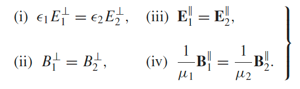 |
B.C. when crossing from medium 1 to medium 2, assuming both are linear material |
| was the one from Maxwell Eq linear material in Chapter 7 Electrodynamics | ||
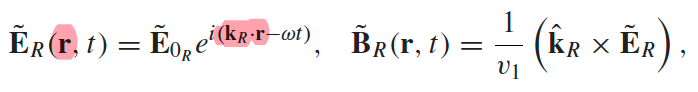
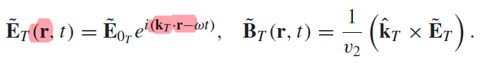
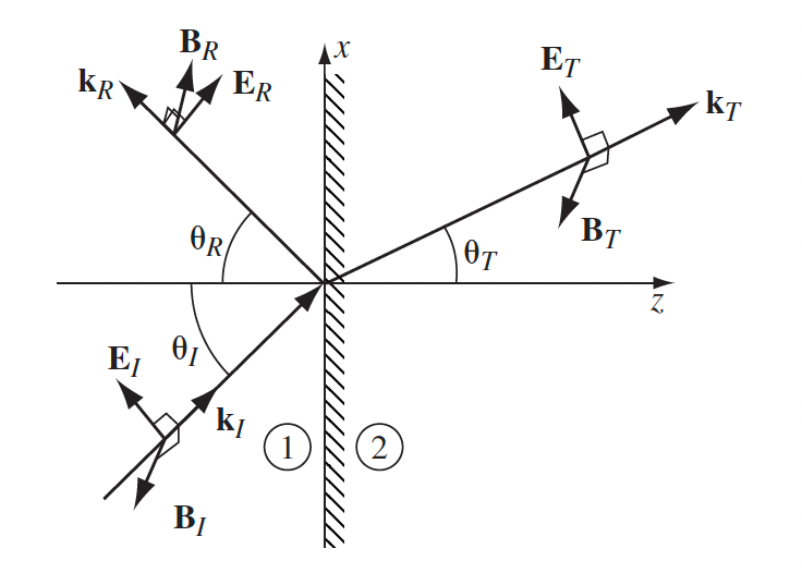
| Setup for EM Wave in Matter + Oblique Incidence | 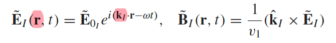 |
still plane waves, but $\mathbf{\tilde{E}}{0_I} = \tilde{E}{0I} \hat{n}{I}$ and we need to consider $\vec{r}$ |
 |
||
 |
||
 |
||
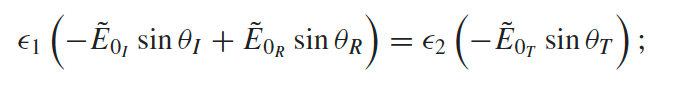
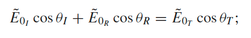
| B.C. for EM Wave in Matter + Oblique Incidence | 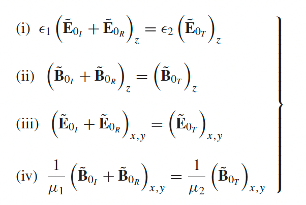 |
derived from the B.C. in material + realizing all the exponential cancels out (see below) |
 |
additional conclusion for the oblique case, derived by realizing the B.C. yields |
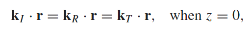
|
| so imagine needing the below to hold for all $\vec{r}$ $A\cos(k_I\cdot \vec{r})+B\cos(k_R\cdot \vec{r})=C\cos(k_T\cdot \vec{r})$ | ||
 |
hence at $z=0$ this has to be true for $\forall x,y$ | |
| $(k_I)_y=(k_R)_y=(k_T)_y$ | from letting $y=0$, | |
| $(k_I)_x=(k_R)_x=(k_T)_x$ | from letting $x=0$ | |
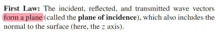 |
derived then aligning $E_I$ into the x-z plane such that $(k_I)_y=0$. Then all other $(k_I)_y=(k_R)_y=(k_T)_y=0$, i.e. all are in x-z plane | |
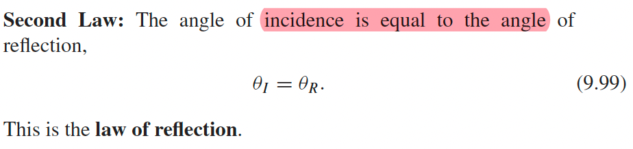 |
from $(k_I)_x=(k_R)_x$, and then realizing that $k_I = k_R$ since $\omega = kv$, both $v,\omega$ is the same for $k_I, k_R$ | |
 |
from $(k_I)_x=(k_T)_x$, and using $v=c/n$ | |
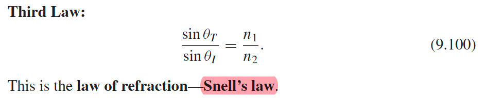
| Solution for EM Wave in Matter + Oblique Incidence | 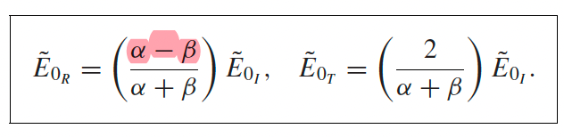 |
$\alpha= \cos\theta_T/\cos \theta_I$, $\beta = (\mu_1v_1)/(\mu_2v_2)$ |
 |
derived from this and below + Snell’s law, which comes from the B.C., assuming $\vec{E},\vec{B}$ are also in the x-z plane (see below) | |
 |
||
 |
||
| Brewster’s angle $\theta_B$ | $\theta_I$ such that there is no reflected wave | e.g. in the case above, when $\alpha=\beta$ |
| Total Internal Reflection | $\theta_I$ such that there is no transmitted energy | |
| Reflection and Transmission index | $R=\frac{I_R}{I_I}, T=\frac{I_T}{I_I}$ | $I=\lang S\rang_z=c\epsilon_0 E_0^2$ for plane waves striking the area |
| $R+T=1$ | basically the input energy = output energy, $I_I=I_R+I_T$ |
Complex Notation in Circuits: consider a given circuit as follows:
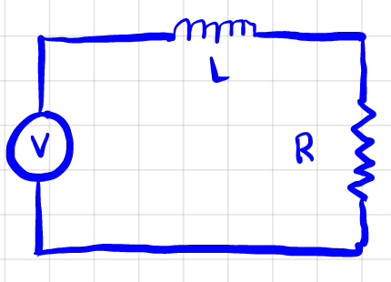
we want to know $I$ flowing in this circuit, if $V=V_0\cos(\omega t)$. We know that the differential equation for $V$ must be
\[V_0\cos(\omega t) - L \frac{dI}{dt} - IR=0\]so $I$ will be sinusoidal in form, and relates to the driving frequency $\omega$. Hence we can consider $I(t)=\tilde{I}_0e^{i\omega t}$:
\[V_0 e^{i\omega t} = L \frac{d}{dt}\tilde{I}_0e^{i\omega t} + R\tilde{I}_0e^{i\omega t}\]then solving you will find:
\[\tilde{I}_0 = \frac{V_0}{i\omega L +R} = \frac{V_0}{\sqrt{\omega^2L^2 + R^2}e^{i\phi}} = = \frac{V_0}{\sqrt{\omega^2L^2 + R^2}}e^{-i\phi}\]note that from this step, we realize that:
- having $L$ in circuit just means a resistance of $i\omega L$
- having capacitance $C$ in circuit, as you will see later, just means a resistance of $i C/\omega$.
- with the above, you can solve circuits without touching differential equations at all, by just treating them as resistors.
for $\tan(\phi)=\omega L/R$, by visualizing $a+ib$ in complex plane. Then you are essentially done since:
\[I(t)= \mathrm{RE}[\tilde{I}_0e^{i\omega t}] =\frac{V_0}{\sqrt{\omega^2L^2 + R^2}}\cos(\omega t - \phi)\]Standing Wave: given a boundary condition that both ends of a wall has to be zero, e.g. $y(x,0)=A\sin (\pi x/L)$
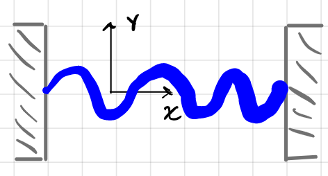
and obviously since this is a string, it needs to satisfy the wave equation
\[\frac{\partial^2 y}{\partial x^2} - \frac{1}{v^2}\frac{\partial^2 y}{\partial t^2} = 0\]then you should guess that the solution $y(x,t)=f(x-vt)+g(x+vt)$ is superposition to two waves:
\[y(x,t) = \frac{A}{2}\left\{ \sin\left[\frac{\pi}{L}(x-vt)\right] +\sin\left[\frac{\pi}{L}(x+vt)\right] \right\}\]How does this work? Two oppositely traveling waves with same frequency forms standing waves = has fixed points!
|  |
EM Wave in Matter: consider the simple example of reflection + transmission for plane waves. Find all amplitudes as a function of $\tilde{E}_I$
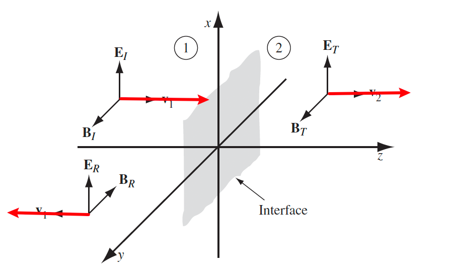
Since these are plane waves, we have
\[\begin{align*} \mathbf{E}_{I}(z,t)&={\tilde{E}}_Ie^{i(k_1z-\omega t)}\hat{x}\\ \mathbf{E}_{R}(z,t)&={\tilde{E}}_Re^{i(-k_1z-\omega t)}\hat{x}\\ \mathbf{E}_{T}(z,t)&={\tilde{E}}_Te^{i(k_2z-\omega t)}\hat{x} \end{align*}\]then the tricky part is realize the $\vec{B}_R$ direction has to be consistent such that $\vec{S}=\frac{1}{\mu_0}\vec{E}\times \vec{B}$ gives $\vec{v}_R$:
\[\begin{align*} \mathbf{B}_{I}(z,t)&=\frac{1}{v_1}{\tilde{E}}_Ie^{i(k_1z-\omega t)}\hat{y}\\ \mathbf{B}_{R}(z,t)&=\frac{\textcolor{red}{-1}}{v_1}{\tilde{E}}_Re^{i(-k_1z-\omega t)}\hat{y}\\ \mathbf{B}_{T}(z,t)&=\frac{1}{v_2}{\tilde{E}}_Te^{i(k_2z-\omega t)}\hat{y} \end{align*}\]then just put them into the B.C. at $z=0$ you get
\[\begin{align*} \vec{E}^{\parallel}_1 - \vec{E}^{\parallel}_2 &= 0 \implies \tilde{E}_I + \tilde{E}_R =\tilde{E}_T \\ \frac{1}{\mu_1}{B}^{\perp}_1 - \frac{1}{\mu_2}{B}^{\perp}_2 &= 0 \implies \frac{1}{\mu_1v_1}\tilde{E}_I -\frac{1}{\mu_1v_1} \tilde{E}_R =\frac{1}{\mu_2v_2}\tilde{E}_T \end{align*}\]then to solve $\tilde{E}_R, \tilde{E}_T$, you can realize that letting $k_i \gets \frac{1}{\mu_iv_i}$ gives you the same set of equations to solve for wave on a string.
Plane Waves with $\vec{J}$
Up to here, we have discussed solutions to wave equations derived
- assuming no charges/currents: now we will have another term in Maxwell’s eq, resulting in a damping term in wave equation (and that $\vec{B}$ is out of phase with $\vec{E}$). You will see this results in $k$ $\to$ $\tilde{k}=k+i\kappa$, so that waves are decaying/not propagating!
- assuming wave $v$ (or rather $\epsilon$) is independent of $\omega$ in material. Before we had $v^2=1/(\epsilon\mu)$ $\to$ you will see $v^2=1/(\tilde{\epsilon}(\omega)\mu)$. Hence this will also affect wave vector $k \to k(\omega)$. In this case, even in a non-conducting material we end up with damping term in solution!
| Condition/Name | Equation | Comments |
|---|---|---|
| Maxwell’s Equation inside a conductor | 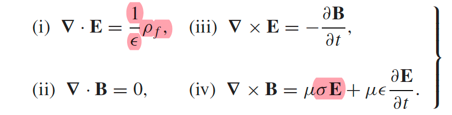 |
basically we have a $\rho_f$ and a $\vec{J}_{free}=\sigma\vec{E}$ inside conductor |
|
derived from this using linear media | |
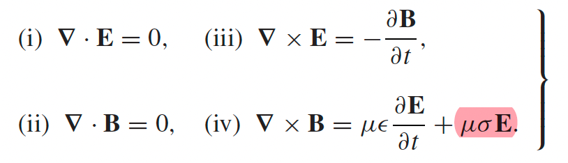
| Wave Equation used Inside Conductor | $\nabla^2\mathbf{E} = \mu\epsilon \frac{\partial^2 \mathbf{E}}{\partial t^2}+\underbrace{\mu\sigma \frac{\partial \mathbf{E}}{\partial t}}_{\text{damping term}}$ | |
| $\nabla^2\mathbf{B} = \mu\epsilon \frac{\partial^2 \mathbf{B}}{\partial t^2}+\underbrace{\mu\sigma \frac{\partial \mathbf{B}}{\partial t}}_{\text{damping term}}$ | ||
 |
this is technically derived from this, i.e. assuming charges has disappeared to boundary | |
| Charge inside conductor | $\rho_f(t) = \rho_f(0)e^{-t/\tau}$ | hence the $\rho_f$ term is ignored (only) when deriving the wave equation |
| derived from the continutiy equation $-\partial\rho_f / \partial t = \nabla \cdot \vec{J}_f$, then using $\vec{J}_f = \sigma \vec{E}$ and $\nabla \cdot \vec{D} = \rho_f$ | ||
| B.C. inside conductor | $\epsilon_1E^{\perp}_1 - \epsilon_2E^{\perp}_2 = \sigma_f$, etc. | derive from the Maxwell’s equation in material, with the presence of both $\rho_f$ and $\vec{J}_f$ |
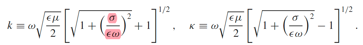
| Solution for Wave in Conductor | $\tilde{k}=k+i\kappa$ | found by plugging our usual solution $\mathbf{\tilde{E}}(z,t)=\tilde{E}_0e^{i(kz-\omega t)}\hat{x}$ into wave equation, and found that $k$ needs to be complex |
| $\mathbf{\tilde{E}}(z,t)=\tilde{E}_0e^{-\kappa z}e^{i(kz-\omega t)}\hat{x}$ | ||
| $\mathbf{\tilde{B}}(z,t)=\tilde{B}_0e^{-\kappa z}e^{i(kz-\omega t)}\hat{y}=\frac{\tilde{k}}{\omega}\tilde{E}_0e^{-\kappa z}e^{i(kz-\omega t)}\hat{y}$ | notice the coefficient $\tilde{k}/\omega$ is complex, i.e. $\vec{B}$ is out of phase with $\vec{E}$. This is derived simply from $\nabla\times \vec{E} = -\partial \vec{B}/\partial t$ | |
| phase difference of $\phi\gets$ converting $\tilde{k}/\omega =Ae^{i\phi}$ | ||
 |
||
| $d\equiv 1/\kappa$ | skin depth, i.e. an indicator of how far wave can penetrate into conductor | |
| $\alpha \equiv 2\kappa$ | absorption coefficient, because intensity is proportional to $E^2$ | |
| $\omega = kv$ holds for the real part of $\tilde{k}$ | because the propagation part is $e^{i(kz-\omega t)}$ | |
 |
if you need to know | |
| Modeling electron’s motion given a driving field | 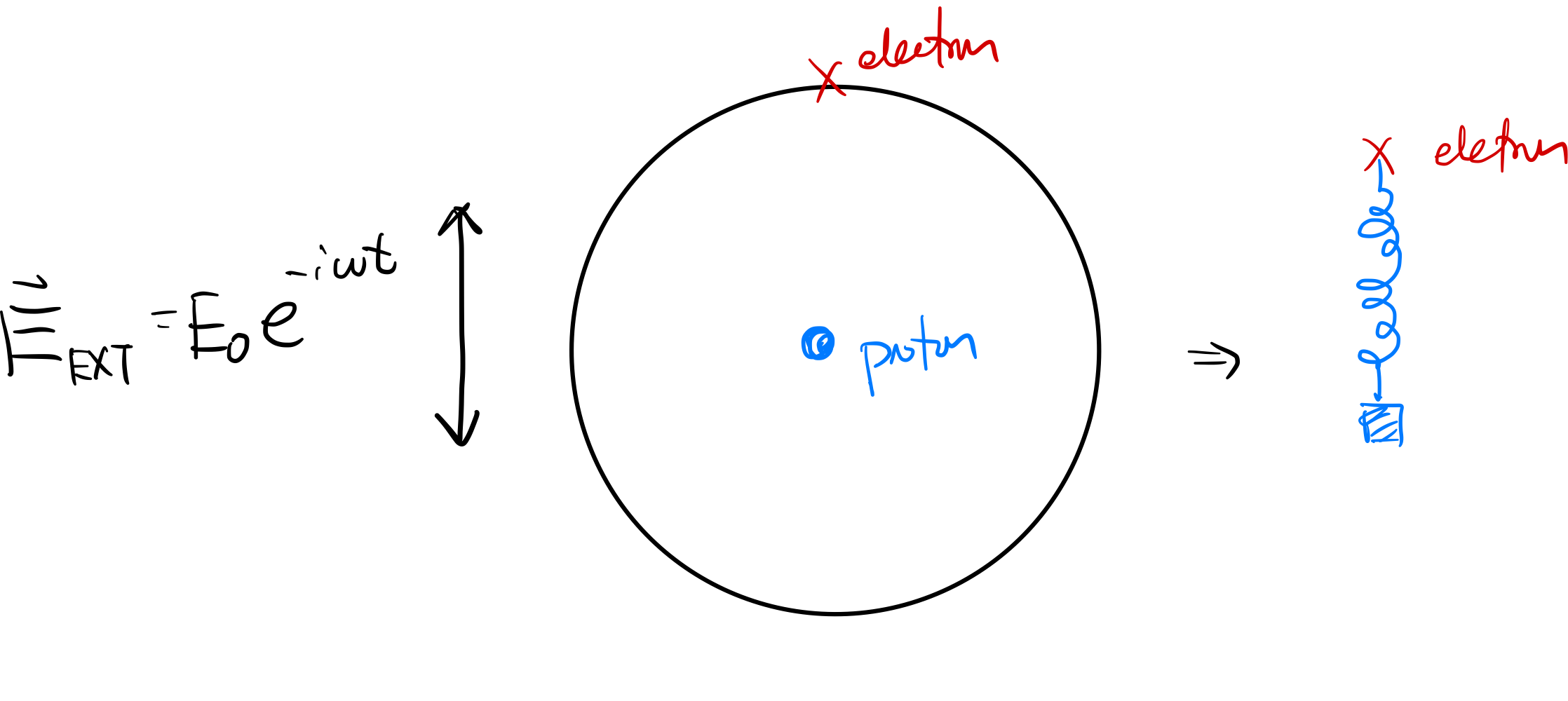 |
|
| $m\frac{d^2x}{dt^2}=\vec{F}{electron}=\vec{F}{E}+\vec{F}{damping}+\vec{F}{SHO}$ | where $\vec{F}E = q\vec{E}{ext}$, damping term $-m\gamma \frac{dx}{dt}$, and SHO force due to the atomic attraction for restoration $\vec{F}_{SHO}=-m\omega_0^2x$ | |
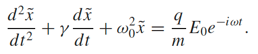 |
the equation of motion | |
| $\omega_0$ will be different for each electron config/also relevant to resonance! | ||
| $\tilde{x}(t)=\tilde{x}_0e^{-i\omega t}$ and $\tilde{x}=\frac{q/m}{\omega_0^2-\omega-i\gamma \omega}E_0$ is complex | solution, by plugging in the steady state $\tilde{x}(t)=\tilde{x}_0e^{-i\omega t}$ | |
| Modeling Polarization given a driving field | 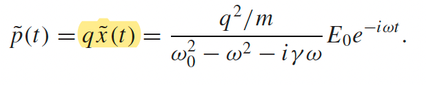 |
notice that $E_0e^{-i\omega t}=\mathbf{\tilde{E}}$ that we supplied |
 |
since $\mathbf{P}=N\tilde{p}$, and $N$ is number of molecules per volume | |
| $\omega_j$ comes from $\omega_0$ being different for different electrons. $f_j$ is the number of electrons having the same $\omega_j$ | ||
| $\mathbf{\tilde{P}}=\epsilon_0\tilde{\chi}_E(\omega)\tilde{E}$ | rewrite the entire wierd term into $\chi_E$ | |
| $\tilde{\epsilon}=\epsilon_0(1+\tilde{\chi}_E) = \epsilon_0\left[ 1+\frac{Nq^2}{m\epsilon_0}\sum_j \frac{f_j}{\omega_j^2 - \omega^2 - i \omega \gamma} \right]$ | after all efforts, the net result is that $\epsilon$ becomes complex and is a function of $\omega$ | |
| Wave Equation after all these | 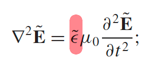 |
|
| $\mathbf{\tilde{E}}(z,t)=\mathbf{\tilde{E}}_0e^{-\kappa z}e^{i(kz-\omega t)}$ | derived from plugging in $\mathbf{\tilde{E}}(z,t)=\mathbf{\tilde{E}}_0e^{i(kz-\omega t)}$ and realizing $\tilde{k} = \sqrt{\tilde{\epsilon}\mu_0}\omega=k+i\kappa$ | |
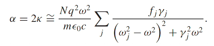
| Resonance frequency | 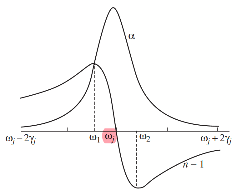 |
so that at $\omega = \omega_j$, absorption peaks = amplitudes of electron oscillation becomes huge |
 |
||
| The above is a dispersive medium | 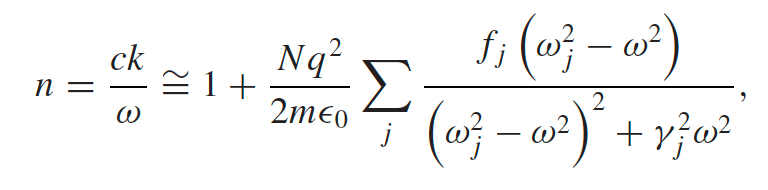 |
$n\to n(\omega)$ index of refraction depends on input wave frequency |
| derived from $\omega = kv,v=c/n$ |
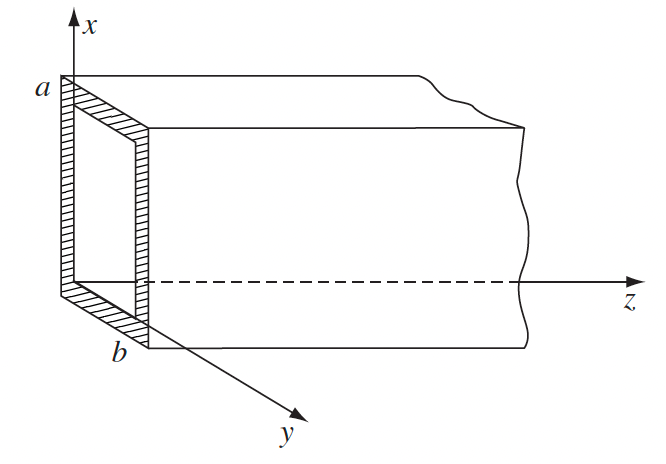
Wave in Wave Guide
No longer plane wave. Now we consider the form
\[\mathbf{E}=\textcolor{red}{\tilde{\mathbf{E}}_0(x,y)}e^{i(kz-\omega t)}\]which has two changes:
-
our old boundary conditions + now the amplitude is a function of $(x,y)$ results in $E$ and $B$ cannot both be perpendicular to $\hat{z}$
-
amplitude as a result also has terms:
\[\mathbf{\tilde{E}}_0(x,y) = \tilde{E}_x(x,y)\hat{x} + \tilde{E}_y(x,y)\hat{y} + \tilde{E}_z(x,y)\hat{z}\]
The net result is that the amplitudes/solution becomes more complicated, e.g. TE waves:
but notice that $\vec{E}$ and $\vec{B}$ still perpendicular to each other
| Condition/Name | Equation | Comments |
|---|---|---|
| Setting up Wave Equation inside Wave Guides | $\mathbf{E}(x,y,z,t)=\textcolor{red}{\tilde{\mathbf{E}}_0(x,y)}e^{i(kz-\omega t)}$ | |
| $\mathbf{B}(x,y,z,t)=\textcolor{red}{\tilde{\mathbf{B}}_0(x,y)}e^{i(kz-\omega t)}$ | ||
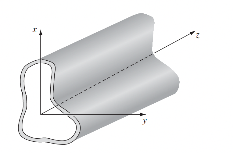 |
why this change? assuming the wave guide is a perfect conductor. | |
 |
then this B.C. means we cannot have plane waves (e.g. try to draw it with a rectangular wave guide) | |
| why this B.C (on the inner surface)? Because $E_{meat}=B_{meat}=0$ for conductor. Then use the usual B.C. from Maxwell’s eq you will get this. | ||
| Generic Solution for Wave in Wave Guide | $\mathbf{\tilde{E}}_0(x,y) = \tilde{E}_x(x,y)\hat{x} + \tilde{E}_y(x,y)\hat{y} + \tilde{E}_z(x,y)\hat{z}$ | our task is just to solve the coefficients |
| $\mathbf{\tilde{B}}_0(x,y) = \tilde{B}_x(x,y)\hat{x} + \tilde{B}_y(x,y)\hat{y} + \tilde{B}_z(x,y)\hat{z}$ | ||
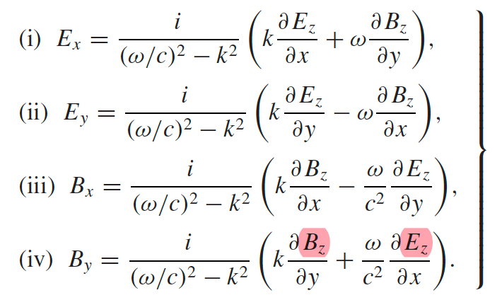 |
by plugging the above into Maxwell’s equation in vacuum. Notice that all are a function $E_z,B_z$ | |
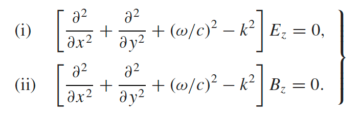 |
so our only task becomes to solve $E_z,B_z$ from this + specific B.C. in a problem | |
| the above is again found in Maxwell Eq. | ||
| so why not transverse wave = $E_z=B_z=0$? Then we would get both the $\nabla \cdot E=0,\nabla \times E=0$, hence $E=-\nabla \phi$ inside. But a conductor has $\vec{E}^{\parallel}{inner}=0$ since $\vec{E}{meat}=0$. Therefore on the surface $\phi=$constant. Then since this satisfies Laplace equation = both mean and max on surface, $\phi$=constant inside as well. Hence $E=0$ entirely. |
||
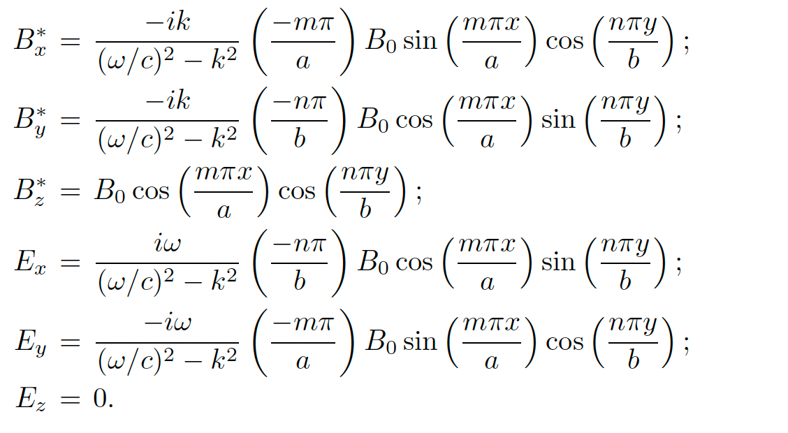
| $TE_{MN}$ waves in Rectangular Wave Guide | $B_z=B_0\cos(k_xx)\cos(k_yy)=B_0\cos(m\pi\frac{x}{a})\cos(n\pi\frac{y}{b})$ | TE because $E_z=0$ hence $E$ is $T$ransverse |
| once $E_z=0$ and $B_z$ is solved, we can solve everything else | ||
| $m=0,1,2,3…$, $n=0,1,2,3,…$, but at least one non-zero so that the solution is not trivial | ||
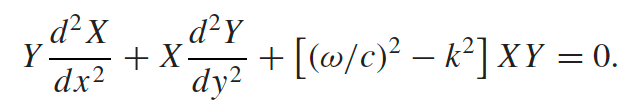 |
derived from using $B_z(x,y)=X(x)Y(y)$ and plugging into the eq for $B_z$ | |
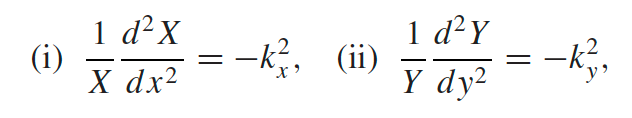 |
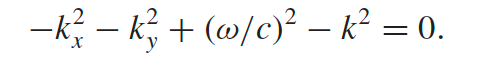
since the first term is only a function of $x$, second only a function of $y$ | |
 |
||
 |
B.C. is in this case is $B_y(y=0)=B_y(y=b)=0$ and $B_x(x=0)=B_x(x=a)=0$ |
|
| Properties of $TE_{MN}$ wave above | $k^2 = \frac{\omega^2}{c^2}\left[ 1-\frac{\omega_{mn}^2}{\omega^2} \right]$, so $\omega_{mn}\equiv \omega_{cutoff}$ | since if $\omega_{cutoff}>\omega$, then $k$ becomes complex and your wave decays in $\hat{z}$/does not propagate |
 |
derived from the equation of $k^2$ from the previous concept | |
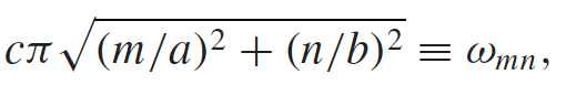
| $v=\omega/k = c/\sqrt{1-(\omega/\omega_{mn})^2}$ | this is $v>c$? Because $v=v_{phase}$. The actual $v_g$ of energy propagation has $v_g <c$ | |
 |
one way to derive the above is $v_g=c\cos(\theta)$, and $v_{phase}=c/\cos\theta$, with knowing $\cos\theta = k/\vert \vec{k}’\vert$ | |
| and $\vec{k}^\prime=k_x\hat{x}+k_y\hat{y}+k\hat{z}$ | ||
| shows what does $k_x,k_y$ represent! | ||
| Group Velocity as velocity of energy transfer | $v_g \equiv d\omega /dk$ | in principle represents velocity of a wave packet |
| $v_g = \frac{\int \lang S\rang_z\cdot d\vec{a} }{\int \lang u\rang_z da}=\frac{\text{energy/time}}{\text{energy/length}}$ | an intuitive “verification” using poynting vector/energy density | |
| $Ae^{i(k+\Delta k/2)z-(\omega + \Delta \omega /2)t}+Ae^{i(k-\Delta k/2)z-(\omega - \Delta \omega /2)t}$ $=Ae^{i(kz-\omega t)}\cos(\frac{\Delta k}{2}z-\frac{\Delta \omega}{2}t)$ $=Ae^{i(kz-\omega t)}\cos (k(z-v_gt))$ |
where it actually comes from = superposing two waves in a specific wave forms a wave packet traveling at $v_g$ (see visualization in the examples section) | |
| $v_g = \Delta \omega /\Delta k$ | in this example |
Group Velocity v.s. Phase Velocity:
In this example, $v_g>v_{phase}$, but in general, most physical systems will have $v_g < v_{phase}$
List of good questions
- Problem 9.7
- (b)(c) dealt with understanding more the B.C. and wave equation
- (d) deals with understanding the complex amplitude $\tilde{A}$
-
Problem 9.17: solid question in understanding B.C. and $\vec{E}$ and $\vec{B}$ with directional $\vec{k}\cdot \vec{r}$.
- Problem 9.39
- (f) is magical, about total internal reflection
- Problem 9.30: what does velocity of “energy propagation” mean, and why group velocity is relevant
Chapter 10 (Retarded) Potentials and Fields
The goal is to find $\vec{E}$ and $\vec{B}$ given some really arbitrary $\rho, \vec{J}$. (Before, we only looked at when $\rho=0$, or when $\vec{J}_f=\sigma\vec{E}$ in a conductor when solving the wave equations.)
In general this is difficult, so here the idea is (like before)
-
solve instead for $\phi, \vec{A}$ under the Lorentz Gauge:
\[\exists \chi,\quad \nabla \cdot \vec{A} + \frac{1}{c^2}\frac{\partial \phi}{\partial t} = 0\]then $\phi, \vec{A}$ satisfies:
\[\begin{cases} \square^2 \phi = - \rho / \epsilon_0\\ \square^2 \vec{A} = - \mu_0 \vec{J} \end{cases}\]where LHS is only the sources, and $\square^2 \equiv \nabla^2 - \frac{1}{c^2} \frac{\partial^2}{\partial t^2}$. Then the solution of $\phi,\vec{A}$ can be guessed:
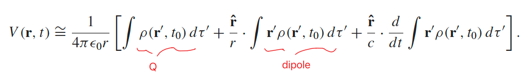
\[\phi(\vec{r},t) = \frac{1}{4\pi\epsilon_0} \int \frac{\rho(\vec{r}',t_r')}{|\vec{r} - \vec{r}'|} d^3r'\\ \vec{A}(\vec{r},t) = \frac{\mu_0}{4\pi} \int \frac{\vec{J}(\vec{r}')}{|\vec{r} - \vec{r}'|} d^3r'\]where $t_r = t - \vert \vec{r} - \vec{r}’\vert /c$ is the retarded time.
-
convert to $\vec{E},\vec{B}$ by $\vec{E} =- \nabla \phi - \frac{\partial \vec{A}}{\partial t}$ and $\vec{B}=\nabla \times \vec{A}$
| Condition/Name | Equation | Comments |
|---|---|---|
| Potential of Fields in electrodynamics | $\vec{E} =- \nabla \phi - \frac{\partial \vec{A}}{\partial t}$ | before in electrostatics we had $\vec{E} =- \nabla \phi$ (from $\nabla \times \vec{E} = 0$)but this no longer works if you consider $\nabla \times \vec{E} = - \partial \vec{B} / \partial t$ |
| $\vec{B}=\nabla \times \vec{A}$ | unchanged | |
| Inhomogenous Wave Equation for $\vec{E},\vec{B}$ given generic $\rho,\vec{J}$ | $\nabla^2 \phi - \frac{1}{c^2} \frac{\partial^2 \phi}{\partial t^2} = - \rho / \epsilon_0$ $\nabla^2 \vec{A} - \frac{1}{c^2} \frac{\partial^2 \vec{A}}{\partial t^2} = - \mu_0 \vec{J}$ |
the first derived from $\nabla \cdot \vec{E}=-\rho / \epsilon_0$, the second derived from $\nabla\times \vec{B}$ and Lorentz Gauge transformation (see below) |
| or equivalently $\square^2 \equiv \nabla^2 - \frac{1}{c^2} \frac{\partial^2}{\partial t^2}$ | ||
| derived from $\nabla^2 \vec{A} - \frac{1}{c^2}\frac{\partial^2 \vec{A}}{\partial t^2} - \nabla(\nabla \cdot \vec{A} + \frac{1}{c^2}\frac{\partial \phi}{\partial t}) = -\mu\vec{J}$ |
which comes from $\nabla \times (\nabla \times \vec{A}) = \nabla \times \vec{B}$ and expand $\vec \times \vec{B}$ using Maxwell’s Eq and $\vec{E} =- \nabla \phi - \frac{\partial \vec{A}}{\partial t}$ | |
| $\vec{A}’ = \vec{A} + \nabla \chi$, and $\phi’ = \phi-\frac{\partial \chi}{\partial t}$ | for some $\chi$ such that the corresponding $\vec{E}'=E$ and $\vec{B}'=\vec{B}$ is unchanged | |
| Lorentz Gauge | $\chi$ such that $\nabla \cdot \vec{A} + \frac{1}{c^2}\frac{\partial \phi}{\partial t} = 0$ | then you easily get $\nabla^2 \vec{A} - \frac{\partial^2 \vec{A}}{\partial t^2} = - \mu_0 \vec{J}$ using the result 2 cells above |
| Retarded Potential | $\phi(\vec{r},t) = \frac{1}{4\pi\epsilon_0} \int \frac{\rho(\vec{r}’,t_r’)}{\vert \vec{r} - \vec{r}’\vert } d^3r’$ | guessed from the Wave equation, just as we guessed from electrostatics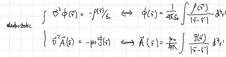 |
| $\vec{A}(\vec{r},t) = \frac{\mu_0}{4\pi} \int \frac{\vec{J}(\vec{r}’)}{\vert \vec{r} - \vec{r}’\vert } d^3r’$ | ||
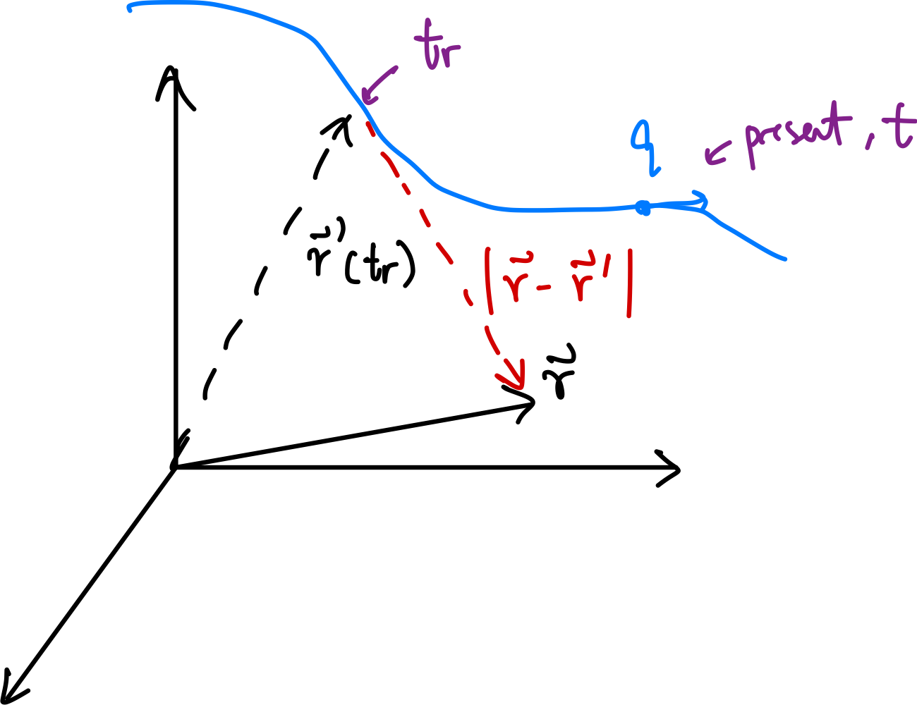
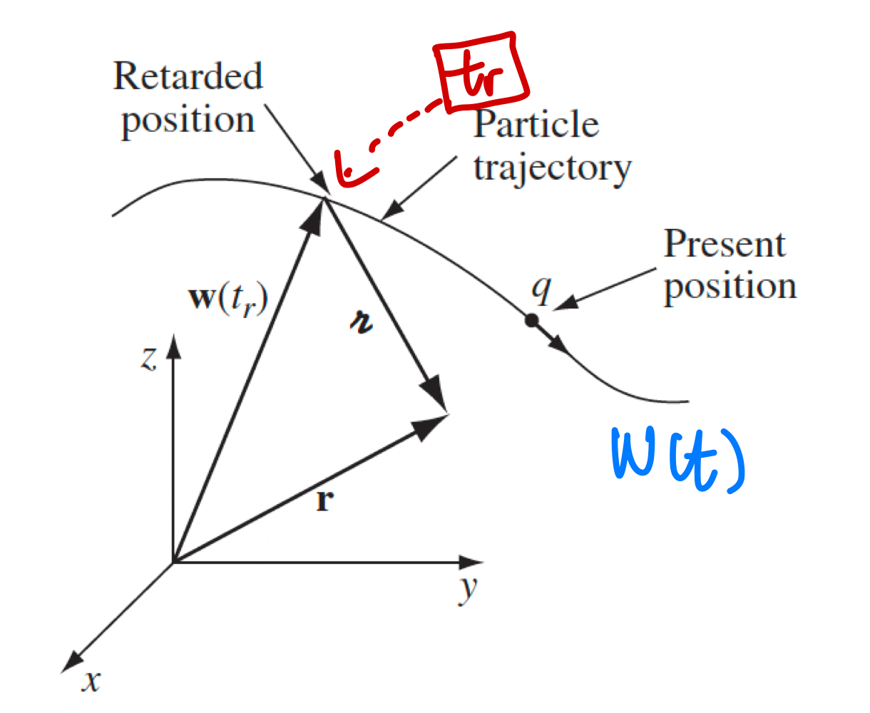
| $t_r = t - \vert \vec{r} - \vec{r}’\vert /c$ | retarded time, or better seen from $\vert \vec{r} - \vec{r}’(t_r)\vert = c(t-t_r)$ | |
 |
||
| has relation to relativity since time is a concern, i.e. in another frame, this retarded time would be different | ||
| Lienard-Wiechert Potentials | $\phi(\vec{r},t) = \frac{1}{4\pi \epsilon_0} \frac{q}{1 - \hat{\mathcal{R}}\cdot \vec{v}(t_r)/c}$ | where $\vec{\mathcal{R}} \equiv \vec{r} - \vec{w}(t_r)$ and $\vec{v}(t_r)$ both are at retarded time |
| $\vec{A}(\vec{r},t) = \frac{\vec{v}(t_r)}{c}\phi(\vec{r},t)$ | derived from length contraction when seomthing is moving towards you, hence $\tau’ = \tau / (1 - \hat{\mathcal{R}}\cdot \vec{v}(t_r)/c)$ is the volume appears to you | |
| generic for a point charge moving in any trajectory $\vec{w}(t)$ | ||
 |
||
| so that $\vert \vec{r}- \vec{w}(t_r)\vert = c(t-t_r)$ | ||
| Fields of a moving point charge | 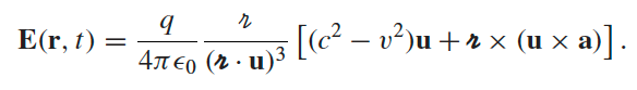 |
where $\vec{u}\equiv c \hat{\mathcal{R}}-\vec{v}$ |
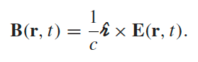 |
derived from the above, since we can compute $\vec{E} = -\nabla \phi - \frac{\partial \vec{A}}{\partial t}$ and $\vec{B} = \nabla \times \vec{A}$ | |
| generic for any trajectory | ||
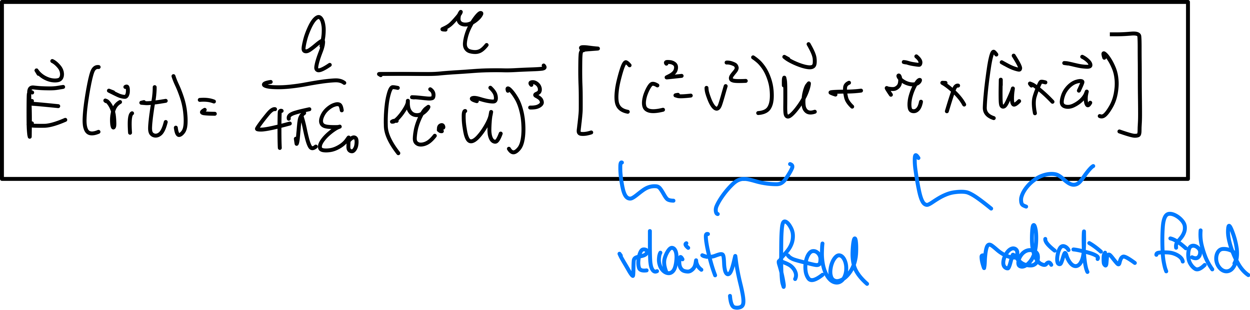 |
velocity field because when $\vert \vec{v}(t)\vert =v$ is constant, then $\vec{E}$ points to its present location 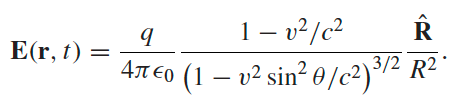 |
|
visually: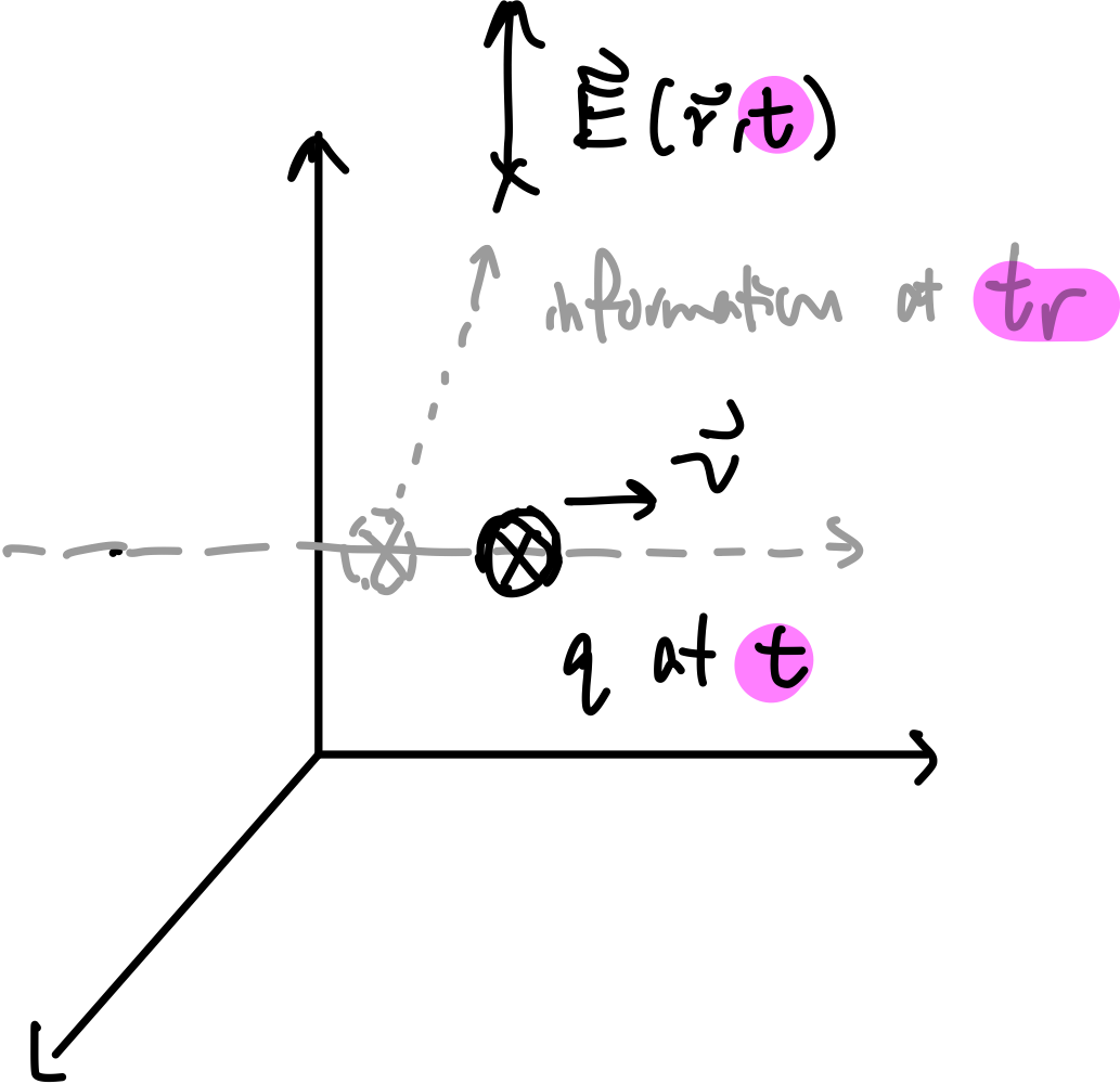 |
||
| radiation field because that term $\propto 1/r$, hence will dominate at large distances (other terms go like $1/r^2$) |
Example Calculation using Lienard-Wiechert Potentials:
Consider a trajectory of a point charge with constant velocity $\vec{w} = vt$. What is its potential $\phi(\vec{r},t)$?
The idea is to express:
\[\phi(\vec{r},t) = \frac{1}{4\pi \epsilon_0} \frac{q}{1 - \hat{\mathcal{R}}\cdot \vec{v}(t_r)/c}\]in terms of $q,v, t$, so that we need to figure out what is $\hat{\mathcal{R}}$. Graphically, we know that it is the position of the charge at $t_r$:
-
find out when is $t_r$:
\[|\vec{r} - vt_r| = c(t-t_r)\]and solve for $t_r$
-
find $\hat{\mathcal{R}}$ since we know $t_r$ and $\vec{w}$:
\[\hat{\mathcal{R}} = \hat{\mathcal{R}}(t_r) = \frac{\vec{r} - vt_r}{c(t-t_r)}\] -
done.
Surprisingly, you will find in the case of constant velocity the corresponding $\vec{E}$ points to the current position of the charge.
Thought Experiment of Velocity Field. Consider a point charge moving at $v$ but suddenly stopped at $T$. You are at $\vec{r}$ and that information hasn’t reach you yet. What would the E field look like in space?
- Since the information that the charge has stopped hadn’t yet reach me (such information propagates as speed of light), then I would experience a field as if the charge is still moving with $v$
- The field when charge has stopped will be simple, and that will propagate at the speed of light
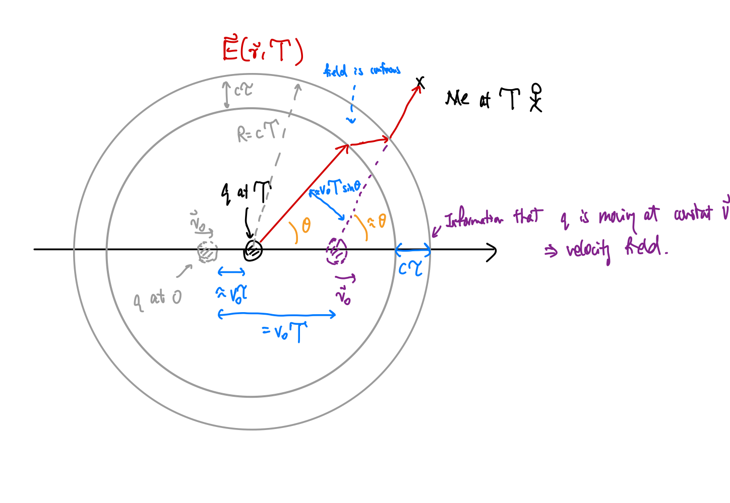
so you get a lot of “kinks”
List of good questions:
- 10.17 = draw the space-time diagram version.
- 10.21 = mind boggling with field of charge at constant velocity.
Chapter 11 Radiation
Radiation studies the parts of $\vec{E},\vec{B}$ that goes like $1/r$, such that even for $r\to \infty$ we get $I=\int \vec{S}\cdot d\vec{A} \neq 0$ meaning energy is radiated and never comes back = permanently lost.
One example of such a field is the “radiation field” discussed in the previous section. This section will basically focus on studying that field.
| Condition/Name | Equation | Comments |
|---|---|---|
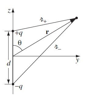
| Electric Dipole Radiation | $\vec{E}_{\text{dipole radiation}} = - \frac{\mu_0 p_0 \omega^2}{4\pi}\frac{\sin(\theta)}{r}\cos(\omega(t-r/c))\hat{\theta}$ | where $p_0 = q_0d$ is electric dipole |
| derived from considering an oscillating dipole constructed with $q(t)=q_0e^{i\omega t}$ | ||
 |
||
| then find its potential $\phi$, discard terms containing any $1/r$, and then compute field $\vec{E}$ to only keep $1/r$ terms | ||
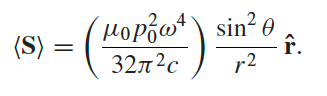 |
by figuring out $\vec{B}$ as well, then $\vec{S} = (1/\mu_0)\vec{E}{\text{rad}}\times \vec{B}{\text{rad}}$ | |
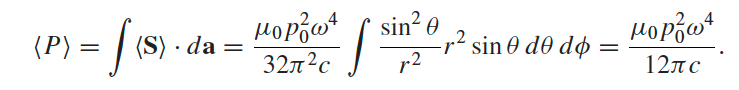 |
total power radiated = energy permanently lost per second | |
| this power is 1) frequency dependent and 2) is consistent with future derivation of generic radiation loss | ||
| Magnetic Dipole Radiation | 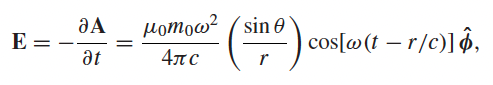 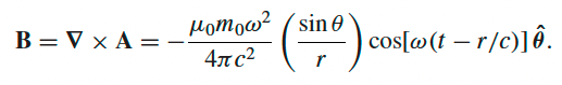 |
derived from considering a current loop such that $\vec{m}(t) = \pi b^2I_0\cos(\omega t)\hat{z}$ |
 |
||
then find its retarded potential $\vec{A}$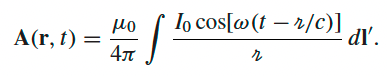 |
||
| and since we know $\phi=0$ , can compute $\vec{E},\vec{B}$ by taking derivatives after knowing $\vec{A}$ | ||
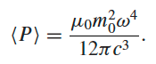 |
derived from finding $\vec{S}$ and taking integral. | |
| very similar to power radiated by electric dipole, but it is much smaller due to $c^3$ term. | ||
| Radiation from Arbitrary Source | $\vec{E}_{\mathrm{rad}}(\vec{r},t) = \frac{\mu_0}{4\pi r}[\hat{r}\times (\hat{r}\times \ddot{\vec{p}})]$ | where $\vec{p}$ is dipole moment for arbitrary distribution $\int r’\rho\,\, d^3r’$ |
| $\vec{B}_{\mathrm{rad}}(\vec{r},t) = \frac{\mu_0}{4\pi rc}[\hat{r}\times \ddot{\vec{p}}]$ | ||
 |
derived from expand the retarded potentials to contain dipole terms (see left), and discard other terms higher than $1/r$ | |
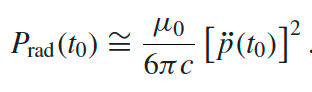 |
finally, the power radiated is given by $\oint \vec{S}\cdot d\vec{a}$ |
Radiation of Point Charges
Now we focus on the specific case of point charges. Since we already know the fields of point charges in Chapter 10, essentially we use $\vec{E},\vec{B}$ from there but focus on $1/r$ terms.
| Condition/Name | Equation | Comments |
|---|---|---|
| Larmor’s Formula | $P_{\mathrm{rad}} = \frac{\mu_0 q^2 a^2}{6\pi c}$ | derived from assuming $v=0$ at $t_r$ so that $\vec{u}=c \hat{\mathcal{R}}$, but actuallly holds well for $v \ll c$ |
| derived from having a point charge moving with trajectory $\vec{w}$, and only taking $\vec{E}{\mathrm{rad}}$ term to compute $\vec{S}{\mathrm{rad}} = (1/\mu_0 c) E_{\mathrm{rad}}^2$ | ||
| then finally $P_{\mathrm{rad}} = \oint \vec{S}_{\mathrm{rad}}\cdot d\vec{A}$ | ||
| this formula is used most often as long as it’s not specified we are at relativistic conditions | ||
| Lienard’s Generalization of Larmor’s Formula | $P_{\mathrm{rad}} = \frac{\mu_0 q^2}{6\pi c}\gamma^6 (a^2 - \left\vert \frac{\vec{v}\times \vec{a}}{c} \right\vert ^2)$ | takes care of the case when $v\approx c$. |
| Radiation Reaction Force | $\vec{F}_{\mathrm{rad}} = \frac{\mu_0 q^2}{6\pi c}\dot{\vec{a}}$ | derived from realizing that $P_{rad}$ loss needs to be taken away from the kinetic energy of a particle. Hence try to find $\vec{F}{rad}\cdot \vec{v} = -P{loss}=-P_{rad}$ |
| since $P_{loss} = \oint \vec{S}\cdot d\vec{A}$ where $\vec{S}$ includes both velocity field and radiation field, here we assume that $P_{loss}=P_{rad}$ by considering a “periodic motion” of the particle os that at $t_2$ it restores its velocity field | ||
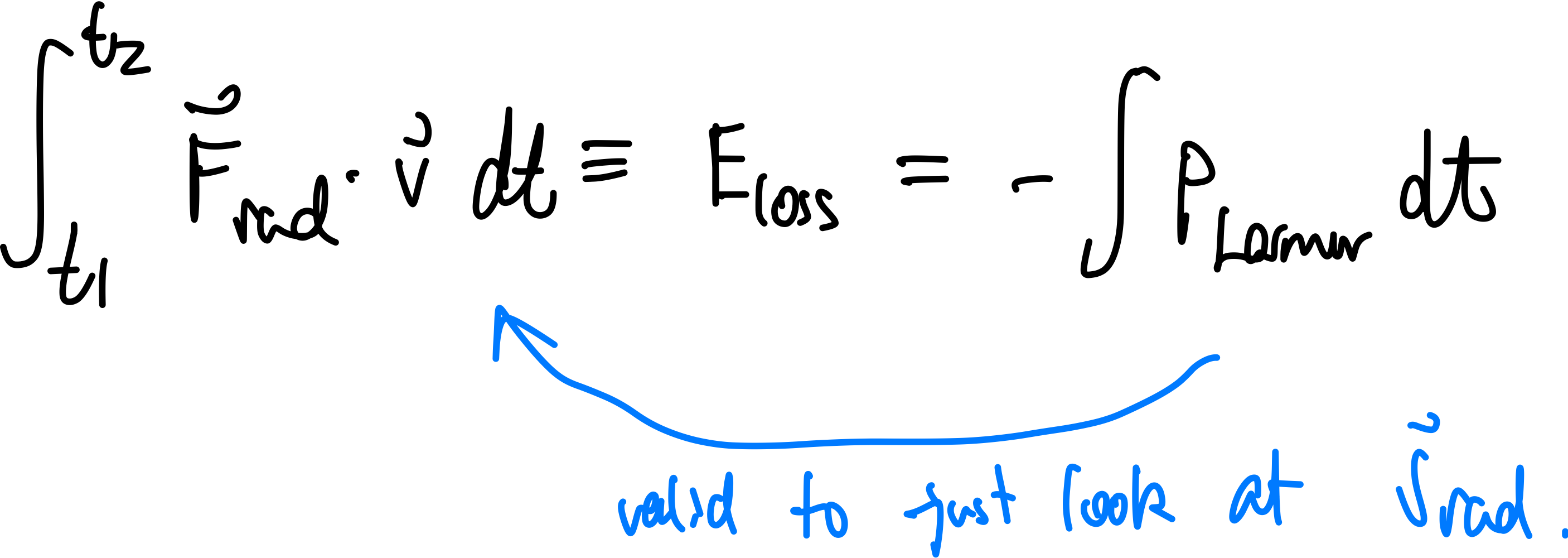 finally substitute in the Larmor’s formula and find $\vec{F}_{rad}$ finally substitute in the Larmor’s formula and find $\vec{F}_{rad}$ |
||
| note that this force is $\propto \dddot{r}!$ |
Using Radiation Reaction to find EoM: since this essentially relates energy loss back to change in acceleration/velocity/position, we can use this if find EoM of an object.
Consider radiation damping of a SHO object, attached to some spring with $\omega_0$ and subject to driving force at $\omega$. Then its EoM look like:
\[m \ddot{x} = F_{\mathrm{spring}} + F_{\mathrm{rad}} + F_{\mathrm{drive}} = - m\omega_0^2 x + m \tau \ddot{x} + F_{\mathrm{drive}}\]where $\tau = \frac{\mu_0 q^2}{6\pi mc}$ from Larmor’s fomula. Then since the solution should be oscillatory, let $x(t) = x_0 \cos(\omega t + \delta)$ to find
\[\ddot{x} = -\omega \dot{x}\]putting this back the EoM becomes
\[m \ddot{x}+ \underbrace{m \omega\tau \dot{x}}_{\text{damping term}} + m\omega_0^2 x = F_{\mathrm{drive}}\]which makes sense as radiation losses energy.
List of good questions:
- 11.14 = how radiation $P_{rad}$ relates to “physical” change in a system
- 11.18 = a bit more into how to use $F_{\mathrm{rad}}$ for energy calculation
- (a) try to derive the EoM and the solution
- 11.19 = normal EoM using $F_{rad}$
Chapter 12 Electrodynamics and Relativity
Iin previous chapters, we understand how to find $\vec{E},\vec{B}$ in some frame. In this chapter we consider, after knowing some $\vec{E},\vec{B}$, how do they transform.
In this chapter you will realize how $\vec{E},\vec{B}$ (and other related quantities such as $\phi, \vec{A}$) can transform into each other when you boost into some inertial frame. Some key findings include
- space-time diagram essentially encodes all features of relativity such as time dilation, length contraction, etc
-
four vectors and four matrices are keys to help you perform transformations easily
- Maxwell’s Eq is already consistent with relativity
Special Relativity and Space Time
Because speed of light is universal in any frame, this basically:
- screwed up spontaneity
- screwed up length = length contration
and all of the above can be intuitively shown using a space-time diagram.
| Condition/Name | Equation | Comments |
|---|---|---|
| space time coordinate | $(ct,x,y,z)=(x^0,x^1,x^2,x^3)$ | |
| Invariant in space time/hyperbolic space | $(ct)^2 - x^2 = (ct’)^2 - x’^2$ | signifies length in hyperbolic space uses this minus sign (instead of $x^2 + y^2 = x’^2 + y’^2$ normally) |
| hence define $x^0 \equiv ct$ | ||
| Lorentz Transformation with Hyperbolic Functions | $x^{0’}=\cosh(u)x^0 - \sinh(u)x$ $x^{‘}=-\sinh(u)x^0 + \cosh(u)x$ $v/c = \tanh(u)$ |
where $x=x^1$ above, assuming the $S’$ frame is moving at $v$. $u$ is also called rapidity |
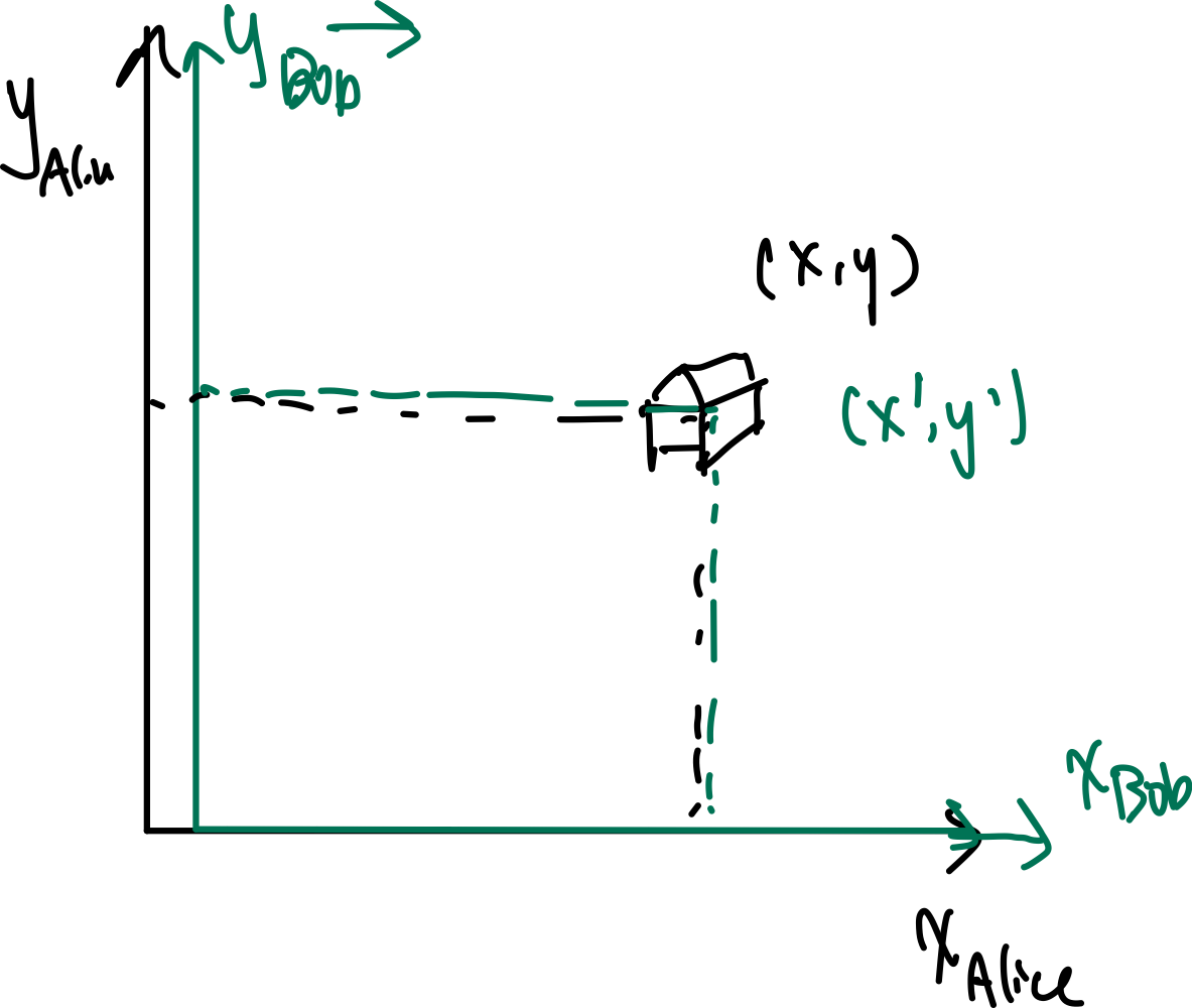 |
||
| e.g. transform into a Bob’s frame moving at $v$ | ||
| this is the more fundamental equations, and makes math also simpler | ||
| Visualization of Rapidity | 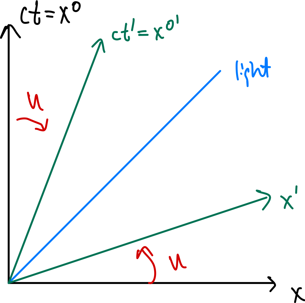 |
derived from thinking about “where to put Bob’s $x^{0^{‘}}$axis” in Alice’s set of axes |
| basically found that $v/c = \mathrm{slope} = \tanh(u)$ | ||
| Lorentz Transformation | $\sinh(u) = \frac{v/c}{\sqrt{1-v^2/c^2}} = \frac{v}{c}\gamma$ $\cosh(u) = \frac{1}{\sqrt{1-v^2/c^2}} =\gamma$ |
derived from $v/c = \tanh(u)$ |
| $t’ = \gamma (t - \frac{v}{c}x)$ $x’ = \gamma (x-vt)$ |
same Lorentz transformation as above | |
| Velocity Addition | $v_{\mathrm{total}}/c = \tanh(u_{\mathrm{total}})=\tanh(u_1+u_2)$ | when you want to find the velocity $v_2$ relative to you, but only given $v_1$ relative to you and $v_2$ relative to $v_1$ |
| $v_{\mathrm{total}} = \frac{v_1+ v_2}{1 + v_1v_2/c^2}$ | same as above, because |
|
| Consequences of living in hyperbolic space | 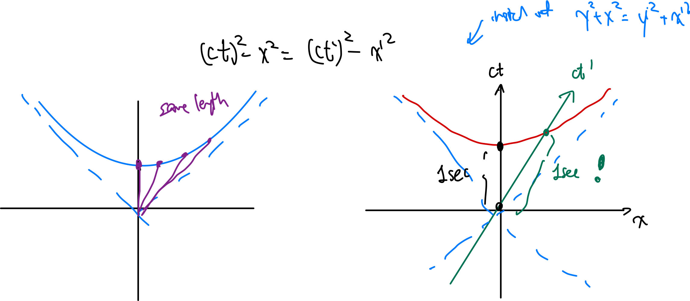 |
lines of same lengths becomes wierd |
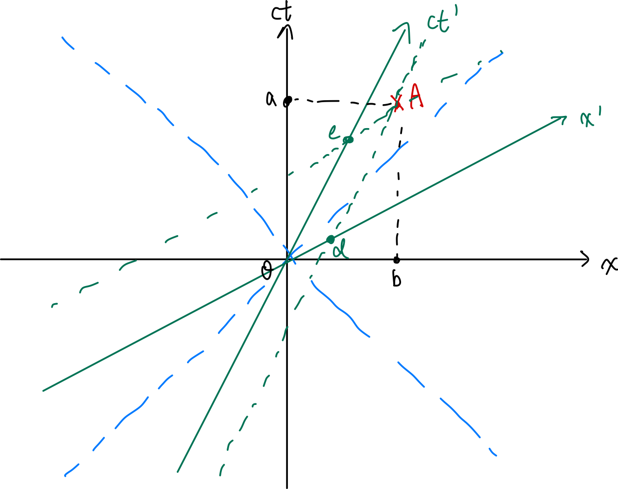 |
vector decomposition in a primed/transformed frame | |
| Relativity of Simultaneity | two events that are simulatenous to one inertial frame are not, in general, simultaneous in another frame | |
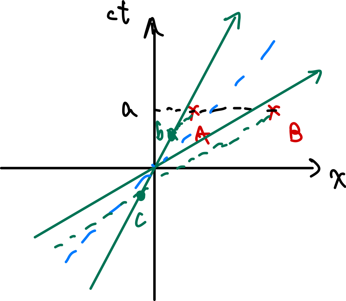 |
event $A,B$ are simultaneous to the unprimed frame, but to the primed frame the two events happened at time $b,c$ respectively | |
| Length Contraction | Things look longer when moving towards you | |
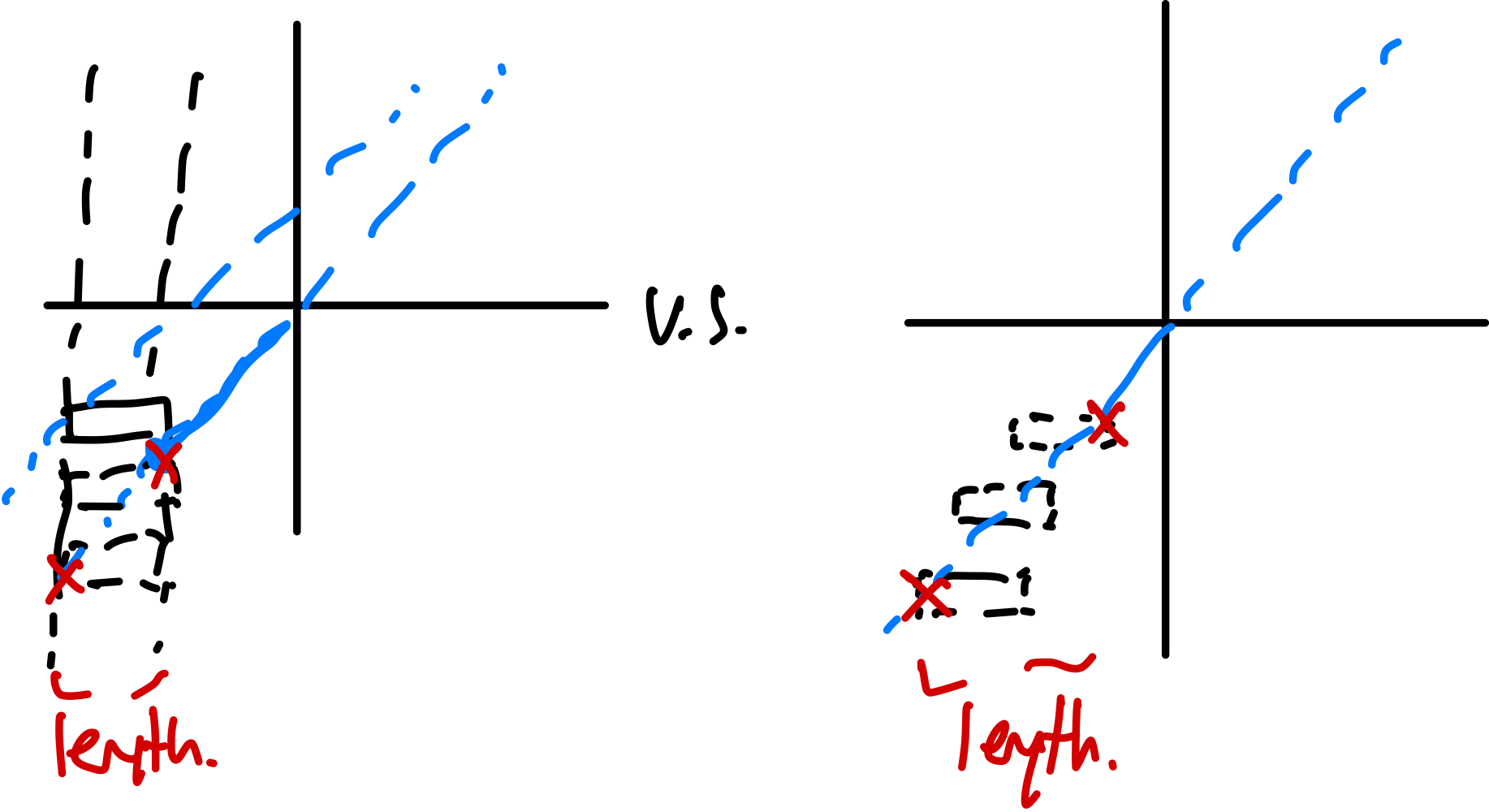 |
note that for things like “length”, we need information to traverse through time, hence the additional photon line | |
| Lorentz Transformation with Matrix | $\begin{bmatrix}x^{0^{‘}}\x^{1^{‘}}\x^{2^{‘}}\x^{3^{‘}}\end{bmatrix} = \begin{bmatrix}\cosh(\theta) & -\sinh(\theta) & 0 & 0\-\sinh(\theta) & \cosh(\theta) & 0 & 0\0 & 0 & 1 & 0\0 & 0 & 0 & 1\\end{bmatrix}\begin{bmatrix}x^{0}\x^{1}\x^{2}\x^{3}\end{bmatrix}$ | |
| $\begin{bmatrix}x^{0^{‘}}\x^{1^{‘}}\x^{2^{‘}}\x^{3^{‘}}\end{bmatrix} = \begin{bmatrix}\gamma & -\gamma\beta & 0 & 0\-\gamma\beta & \gamma & 0 & 0\0 & 0 & 1 & 0\0 & 0 & 0 & 1\\end{bmatrix}\begin{bmatrix}x^{0}\x^{1}\x^{2}\x^{3}\end{bmatrix}$ | where $\beta = v/c$ | |
visually, boosting from $S$ to the moving$S’$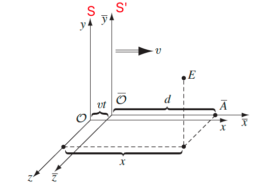 |
||
| “Inverse” Lorentz Transformation | $\begin{bmatrix}x^{0}\x^{1}\x^{2}\x^{3}\end{bmatrix} = \begin{bmatrix}\cosh(\theta) & \sinh(\theta) & 0 & 0\\sinh(\theta) & \cosh(\theta) & 0 & 0\0 & 0 & 1 & 0\0 & 0 & 0 & 1\\end{bmatrix}\begin{bmatrix}x^{0^{‘}}\x^{1^{‘}}\x^{2^{‘}}\x^{3^{‘}}\end{bmatrix}$ | equivalent of the above but $S$ moving to the left relative to $S’$ |
| Four vectors | $x^\mu \equiv \begin{bmatrix}x^{0}\x^{1}\x^{2}\x^{3}\end{bmatrix}$ | (same as above cell, but different representation) |
| $x^{\mu^{‘}} = \Lambda_\nu^\mu x^\nu \equiv \sum_\nu \Lambda_\nu^\mu x^\nu$ | where $\nu$ is row, $\mu$ is column of the matrix. | |
| in this case, the summation notation is equivalent to perform matrix multiplication | ||
| any valid four vectors need to satisfy this transformation rule | ||
| Minkovski metric | $\Delta x_\mu = \eta_{\mu\nu}\Delta x^\nu$ | lowering index |
| $\Delta x^\mu \cdot \Delta x^\mu = \Delta x_\mu \Delta x^\mu = \text{invariant} = (c^2t^2 - d^2)$ | where $d^2 = x^2 + y^2 + z^2$ (as mentioned before, this is length in space-time) | |
| $\eta_{\mu\nu} = \begin{bmatrix}1 & 0 & 0 & 0\0 & -1 & 0 & 0\0 & 0 & -1 & 0\0 & 0 & 0 & -1\\end{bmatrix}$ | mostly negative convention, called the metric | |
| $\eta_{\mu\nu}=\eta^{\mu\nu}$ | the RHS is used to raise the index | |
visually, $I$ is the invariant: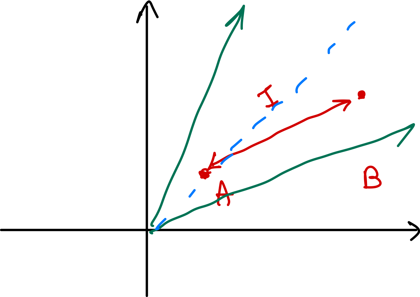 |
||
| Time like events | when $I=(c^2t^2-d^2) > 0$ | |
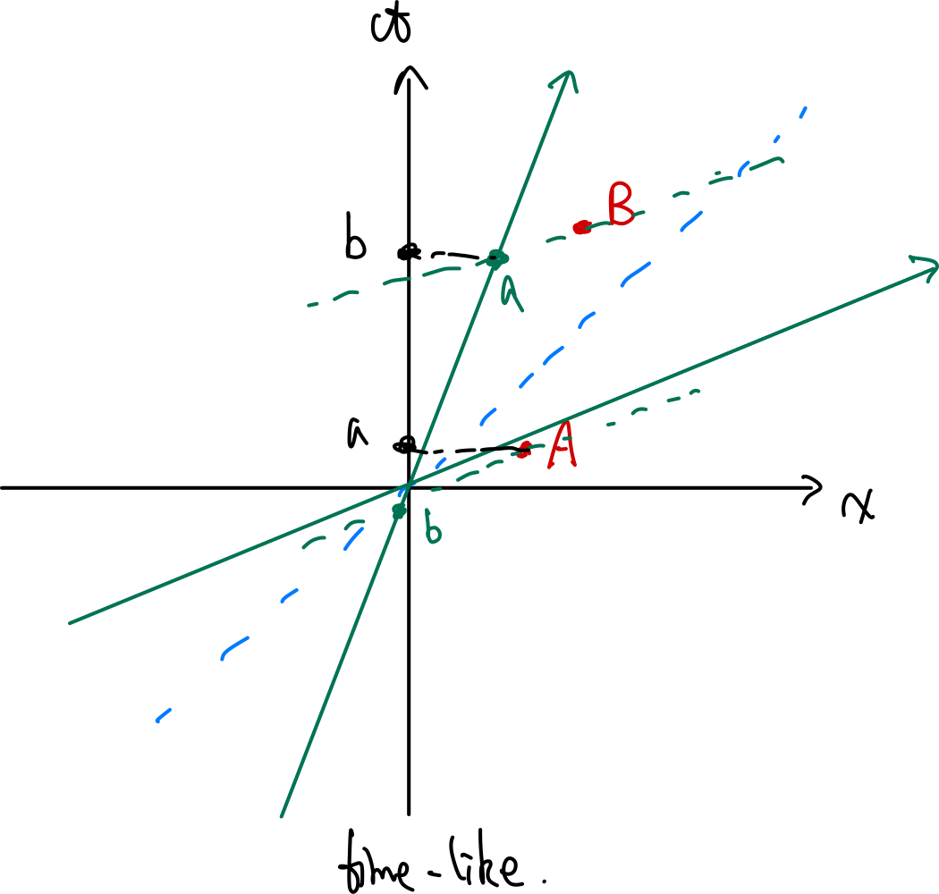 |
if $A$ happened before $B$ in one frame, this order must hold in any other frame = causality is maintained | |
| Space like events | when $I=(c^2t^2-d^2) < 0$ | |
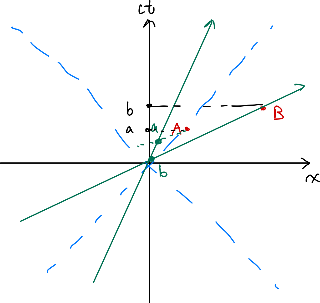 |
no causality, and the order of event is no longer absolute |
Graphical Example of Time Dilation
In a primed frame, let an event happened at $\Delta t’ = 1$ hour. The same event to an unprimed frame would have happened at $\Delta t > \Delta t’$:
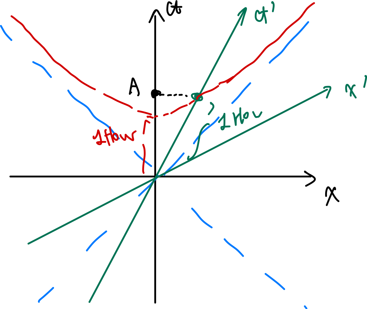
Relativistic Mechanics
Now, we focus on how “definitions” of energy, momentum, and conservation principles “changed” when we consider relativity, i.e. do they hold when I transformed into another inertial frame? In sum:
-
energy/momentum redefined through proper time
-
relativistic energy and momentum is conserved
why need to “redefine”? It turns out using proper time = can write those quantities into four vectors = much easier to transform = nice properties follows such as conservation of relativistic energy.
| Condition/Name | Equation | Comments |
|---|---|---|
| Transforming ordinary velocity | $v_x = v^1 = \frac{\Delta x^1}{\Delta t} = c\frac{\Delta x^1}{\Delta t} = c \frac{\cosh(\theta)\Delta x^{0’} + \sinh(\theta) \Delta x^{1’}}{\sinh(\theta)\Delta x^{0’} + \cosh(\theta) \Delta x^{1’}}$ | given $v^{1’}$ to figure out $v^1$ needs to transform both $\Delta x^1\gets \Delta x^{1’}$ and $\Delta t \gets \Delta t’$ |
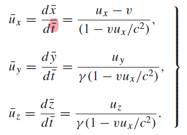 |
“consequence” of using ordinary velocities | |
| Proper Time | $\Delta \tau$ instead of $\Delta t$ | |
| $\Delta x_\mu \Delta x^\mu \equiv \Delta s^2 \equiv (c\Delta \tau)^2$ | $\Delta \tau$ is time for a photon to travel $\Delta s$, which is invariant under transformation | |
| $\Delta \tau = \Delta t / \gamma$ | derived from realizing $\Delta \vec{x}\cdot \Delta \vec{x} = (v\Delta t)^2$, and that $\Delta x_\mu \Delta x^\mu = c^2\Delta t^2 - \Delta \vec{x}\cdot \Delta \vec{x}$ | |
| this is actually quite useful later on since it means $d \tau / dt = 1/\gamma$ | ||
| Four velocity | $\frac{\Delta x^\mu}{\Delta \tau}\equiv u^\mu = \gamma (c, \vec{v})$ | is a four vector and transforms with $u^{\mu^{‘}} = \Lambda_\mu^\mu u^\nu$ |
| $\vec{v}$ is ordinary velocity | ||
| $u_\mu u^\mu = \gamma^2(c^2 - v^2)=c^2$ is invariant | ||
| Four momentum | $P^\mu \equiv c\cdot m u^\mu$ | we put an extra $c$ so that we get the below |
| $P^\mu = (\gamma mc^2 , c \gamma \vec{p}) = (E_{relat}, c\vec{p}_{relat})\equiv (E, c \vec{p})$ | relativistic energy and momentum | |
| you can show that $E_{rela} = \gamma mc^2$ includes both $mc^2$ and $(1/2)mv^2$ by expanding $\gamma$. It really is “total energy” | ||
| $P_\mu P^\mu = (mc^2)^2$ is invariant | ||
| Mass-Energy equivalence | $P_\mu P^\mu = E^2 - p^2c^2 = m^2c^4$ | all comes naturally using four vector |
| Energy/Momentum of Photon | $E=pc$ | special case since $m = 0$, then the formula $E=mc^2 \gamma$ doesn’t work as both numerator and denominator has zero |
| hence comes from Mass-energy equivalence | ||
| Conservation of relativistic energy and momentum | $P^\mu_{\mathrm{IN}}=P^\mu_{\mathrm{OUT}}$ | note that being invariant has nothing to do with being conserved (e.g. mass is invariant but not conserved = some goes into energy) |
| Center of mass energy | find by $P_\mu P^\mu = P_{CM_\mu} P_{CM}^\mu =E_{CM}^2$ | where $P_{CM}^\mu = (E_{CM},0)$ |
| utilizing the fact that $P_\mu P^\mu$ is invariant in any frame | ||
| Relativistic Force | $\vec{F} = \frac{d\vec{P}_{relat}}{dt} = \frac{d}{dt} \frac{m\vec{v}}{\sqrt{1-v^2/c^2}}$ | we use the relativistic momentum but ordinary time |
| as a result, transformation looks somewhat ugly | ||
| but only this form is consistent with the force in $\vec{F}=q(\vec{E}+\vec{v}\times \vec{B})$ | ||
| can use this to compute trajectory of particles under some force |
Mass is not conserved:
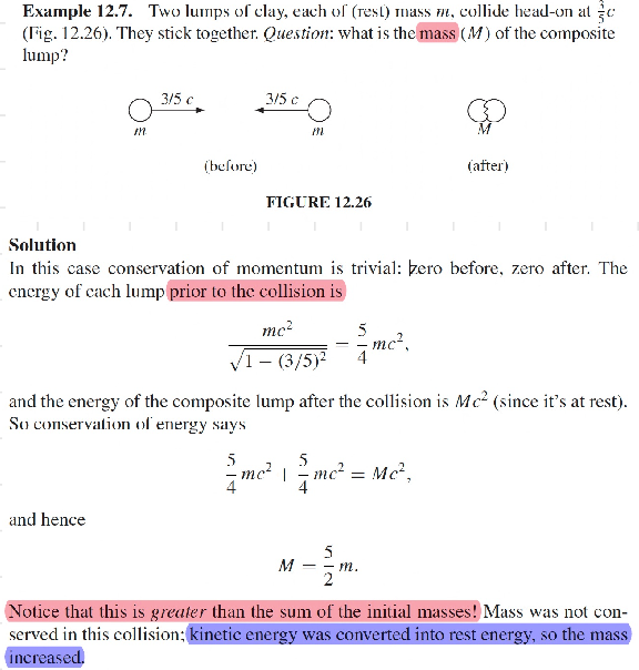
Conservation of Energy and Momentum using Four vectors
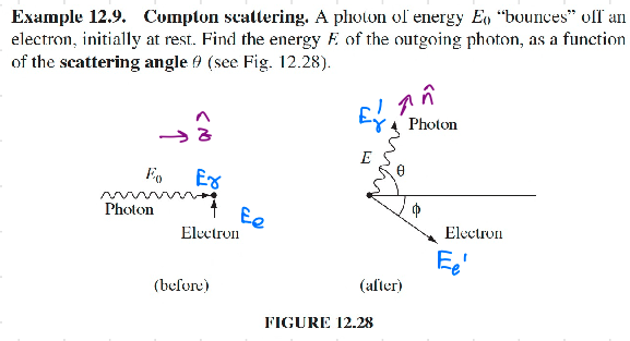
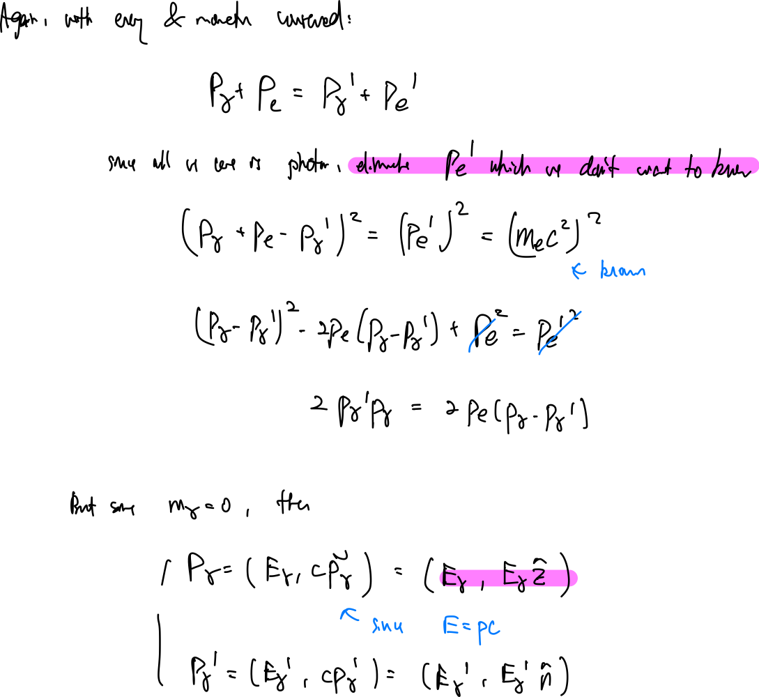

Trajectory of a particle given some force. Let an object move from rest at $t=0$ under constant force. what is $x(t)$ over time?
The key is to think that $\vec{F} = d\vec{p}_{relat}/dt$, which tells you what is $\vec{v}(t)$, then you can integrate to get $x(t)$
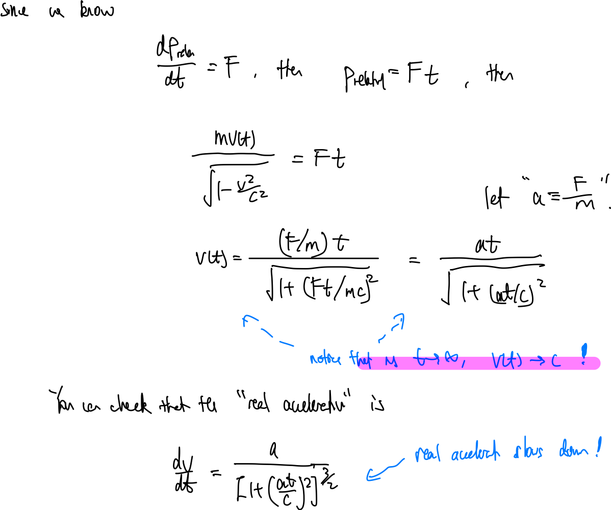
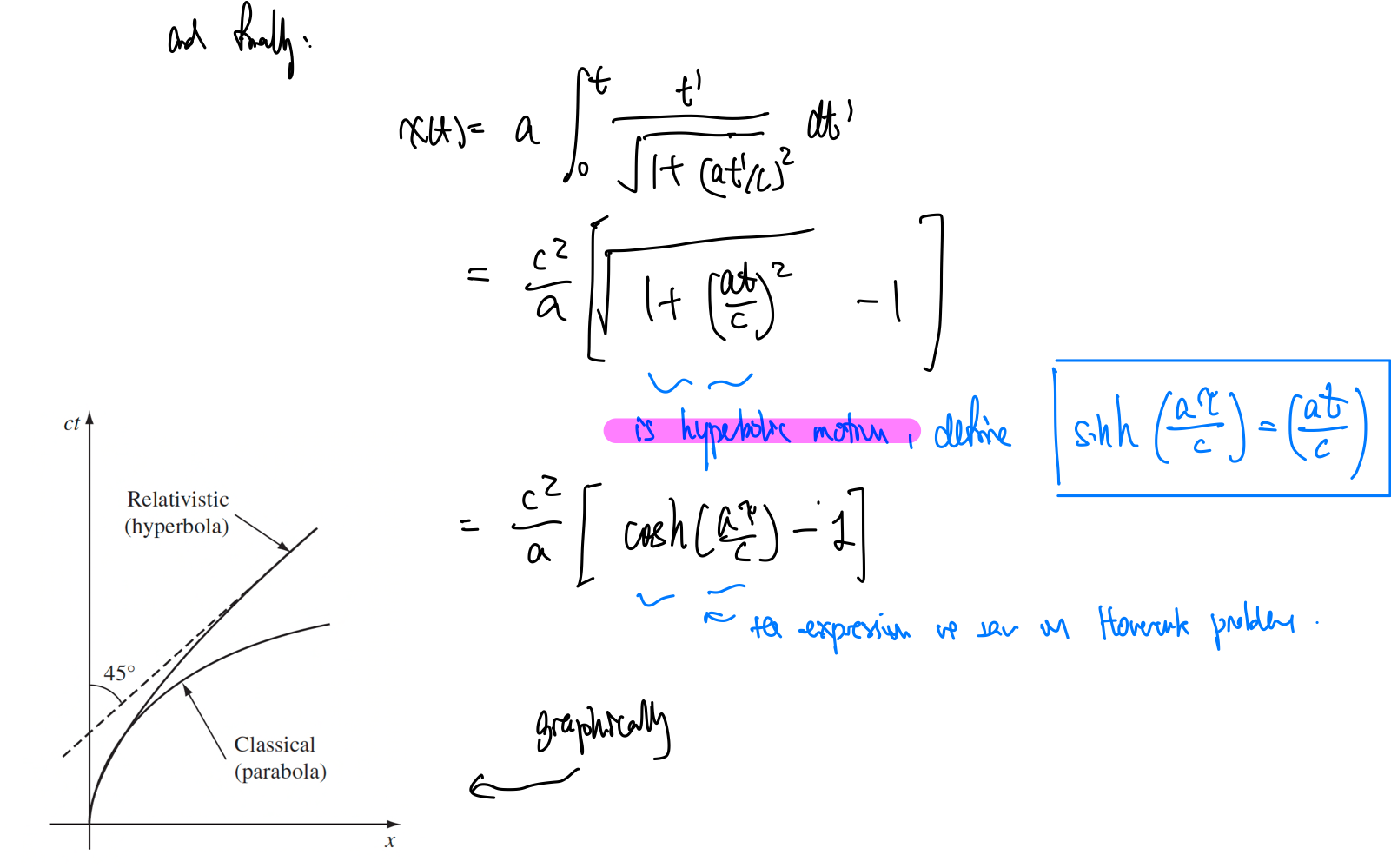
Relativistic Electrodynamics
Here you will see that:
- magnetic process is a relativistic effect of electric process, i.e. you can have magnetic field in one frame, boost in another frame, and obtain no magnetic field but electric field (in the end what matters is the actual force = affecting particles’ motion)
- Maxwell’s equation is naturally relativistic
- we will show the above by re-writing (no new physics) every related Maxwell quantities in four vector/matrix formation
| Condition/Name | Equation | Comments |
|---|---|---|
| Example of mixing $\vec{E}$ and $\vec{B}$ | $F_M = \frac{1}{\gamma} F_E’$ | |
frame $S$: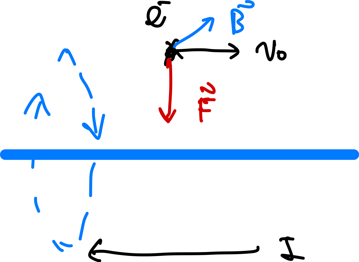 |
a charge moving with $v$. Wire is charge neutral hence $\vec{E}=0$ | |
frame $S’$: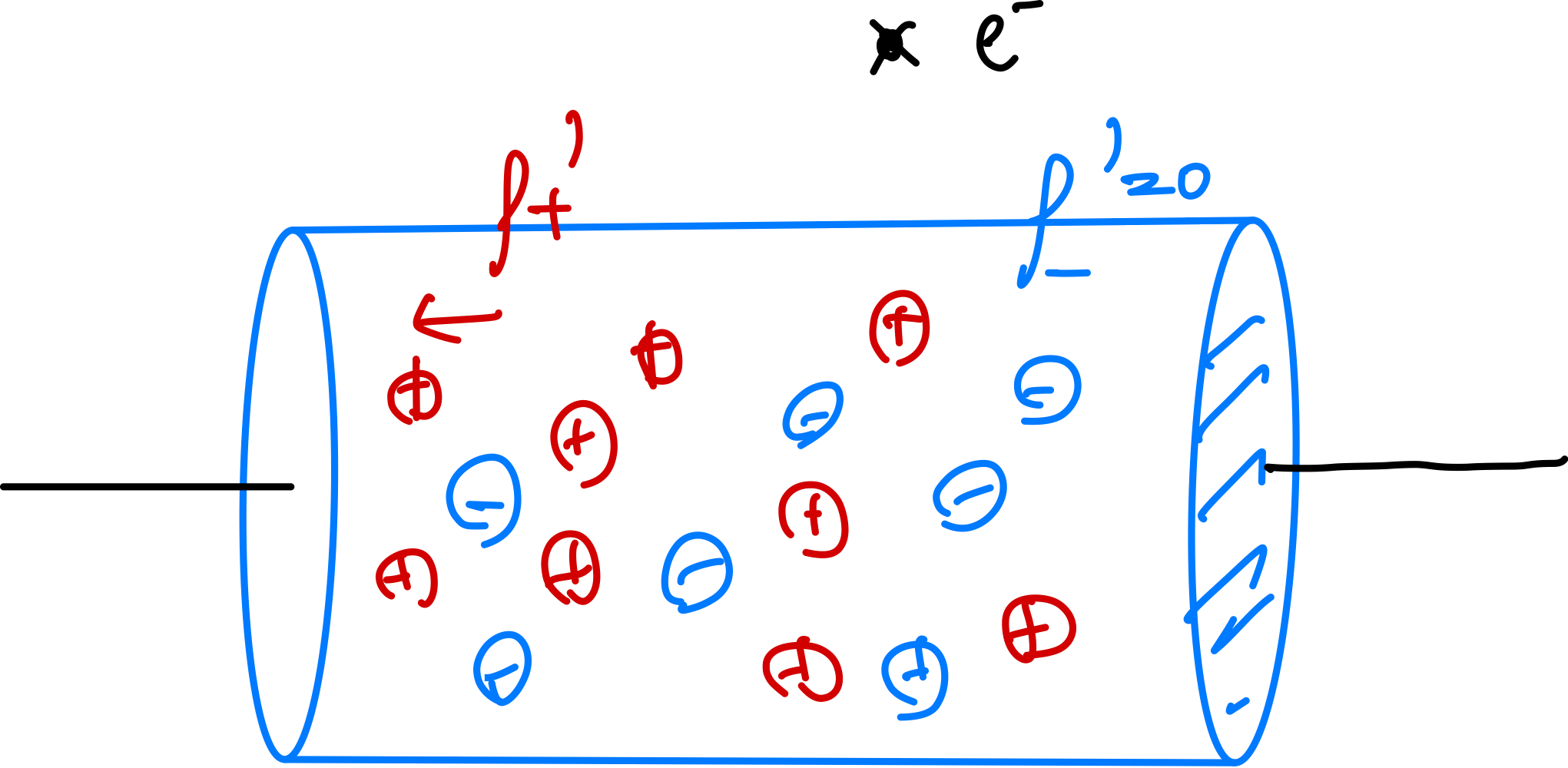 |
boost into the charge’s frame, now $\vec{v}\times \vec{B}=0$, but $\vec{E}\neq 0$ now! | |
| because the charge density changes: $\rho = #\text{charges}/(\Delta x \Delta y \Delta z)$, and one of the dimension experience Lorentz contraction | ||
| as a result line density $\lambda = (\rho_+’ - \rho_-‘)A \neq 0$ in frame $S’$, hence obtain electric field | ||
| essentially, what changed under boosts are the charge densities | ||
| Transformation of $E,B$ field | 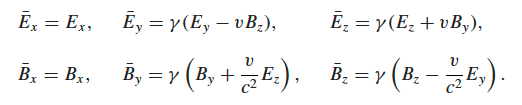 |
when boosting into some frame with $v$ |
| derived from parallel plate, and arguing how surface charge density is the only thing that changed | ||
| Transformation of $E,B$ field in Tensor Notation |  |
equivalent of the above!! |
| note that this summation is different from matrix multiplication | ||
| Field Tensor | 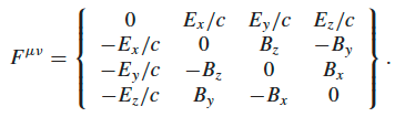 |
|
| $F^{\mu\nu’} =\Lambda^{\mu}\lambda \Lambda{\sigma}^{\nu}F^{\lambda \sigma}$ | in summation notation | |
| $F^{\mu\nu} F_{\mu\nu}= 2(E^2/c^2 - B^2)$ is invariant | ||
| Dual of Field Tensor | 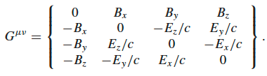 |
|
| Four current and conservation of charges | $J^\mu \equiv (c\rho, \vec{J})$ | |
 |
is equivalent of 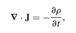 |
|
| (helpers) Transformation of Derivatives | $\frac{\partial }{\partial x^\mu} \equiv (\frac{\partial }{\partial x^0}, \frac{\partial }{\partial x^1}, \frac{\partial }{\partial x^2}, \frac{\partial }{\partial x^3}) \equiv \partial_\mu$ | lower derivatives for upper index |
 |
transformation of derivatives | |
derived from  |
||
 |
raising derivatives | |
| Derivatives to D’ Lambertian |  |
|
| Re-Expressing Maxwell’s equation | $\frac{\partial F^{\mu\nu}}{\partial x^\nu} = \partial_\nu F^{\mu\nu} = \mu_0 J^\mu$ $\frac{\partial G^{\mu\nu}}{\partial x^\nu} = \partial_\nu G^{\mu\nu} = 0$ |
same as all four of Maxwell’s equation |
for example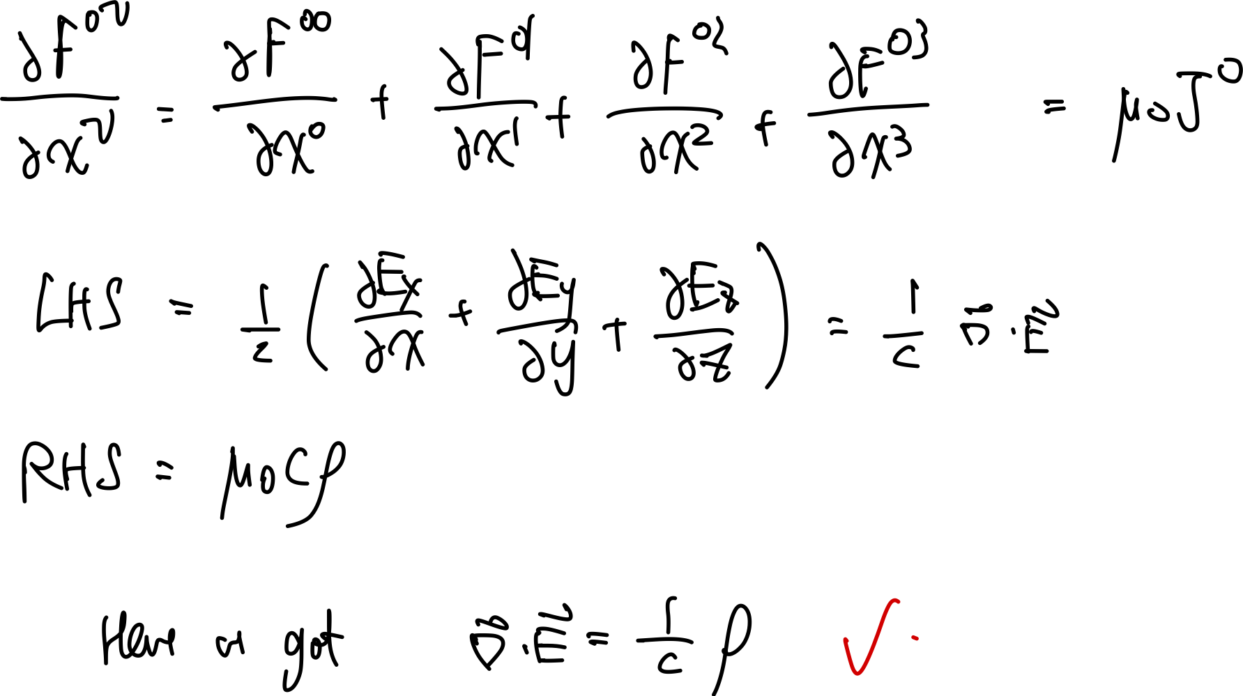 |
||
| Re-Expressing Lorentz Force | $K^\mu \equiv \frac{dp^\mu}{d\tau}$ | proper force (instead of $\vec{F} = \frac{d\vec{P}_{relat}}{dt}$) |
| $K^\mu = q u_\nu F^{\nu\mu}$ | equivalent of $\vec{F}= q(\vec{E} + \vec{v}\times \vec{B})$ | |
for example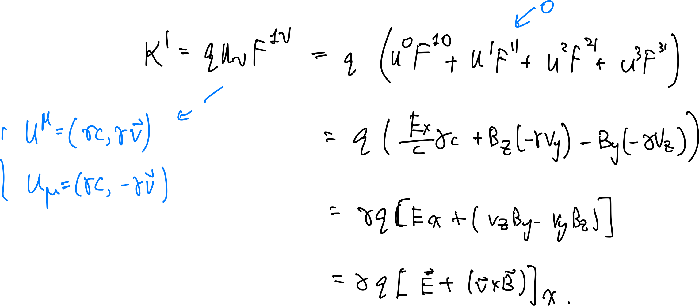 |
||
| Re-Expressing Potentials | $A^\mu = (\phi/c, \vec{A})$ | four potential |
| $F^{\mu\nu} = \frac{\partial A^\nu}{\partial x_\mu}-\frac{\partial A^\mu}{\partial x_\nu} = \partial^\mu A^\nu - \partial^\nu A^\mu$ | equivalent to $\vec{E} =- \nabla \phi - \frac{\partial \vec{A}}{\partial t}$ and $\vec{B}=\nabla \times \vec{A}$ | |
notice that this is upper index derivative. In a mostly positive metric you get an extra minus sign for $x^0$ term: |
||
| Re-expressing Gauges and “Wave Equation” | $A^\mu \to A^\mu + \frac{\partial \chi}{\partial x_\mu}$ | the above hints at Gauge transformation, won’t change $F^{\mu\nu}$ |
| $\partial^\nu\partial_\mu A^\mu = \square^2 A^\mu = -\mu_0 J^\mu$ | equivalent to $\square^2\phi = - \rho / \epsilon_0$ $\square^2 \vec{A} = - \mu_0 \vec{J}$ |
List of good questions:
-
12.6 = need to understand the consequence of $t\neq t’$
-
12.8 = not entirely sure how space-time works, potentially needed to deal with hyperbolic space
- one take-away from this is: let me be traveling at $v$ w.r.t. some stationary observer. When I travelled $d’ = v \Delta t’$ for $\Delta t’$ in my frame, to other people they think I travelled $d=v \Delta t \neq d’$! The “real distance” should be $d’=v\Delta t’$.
-
12.13 = how to draw simultanoues event
- two events simultaneous on a reference frame $\neq$ an observer will see them simultaneously (i.e. no light ray)
-
12.36 = get object velocity from relativistic energy
-
professor added question: how rapidity can be used with energies
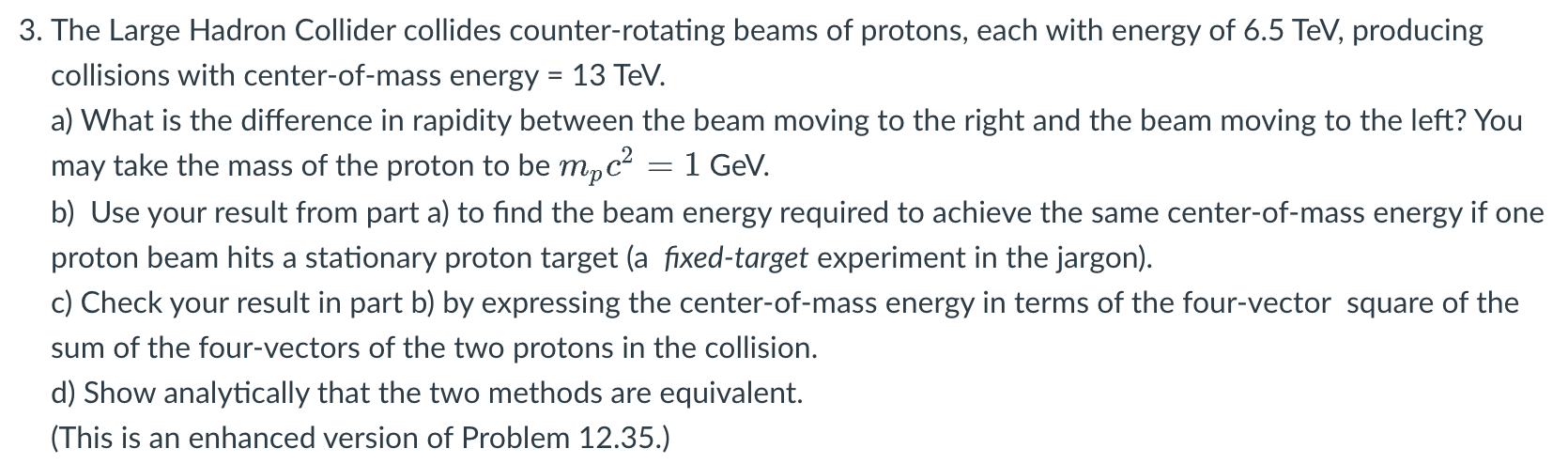
-
professor added question: Lorentz transfomation and what does a free-fall trajectory look like
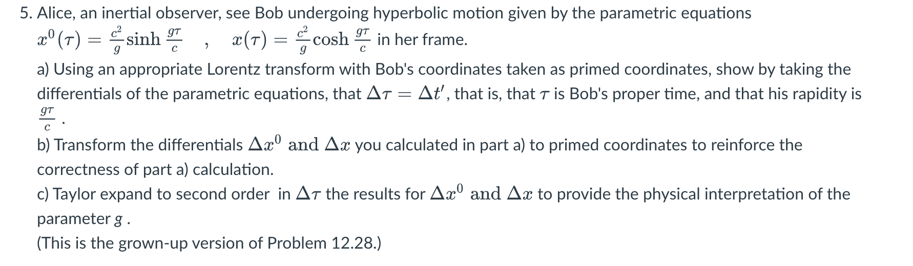
-
professor added question of how to transform momentum
-
12.51: $F_{\mu\nu}F^{\mu\nu}$ is really just summing index, not matrix multiplication