Stanford Reinforcement Learning:

course video: https://www.youtube.com/watch?v=FgzM3zpZ55o&list=PLoROMvodv4rOSOPzutgyCTapiGlY2Nd8u&index=1
assignments: https://github.com/Huixxi/CS234-Reinforcement-Learning-Winter-2019
slides: https://web.stanford.edu/class/cs234/CS234Win2019/schedule.html

Introductions

Reinforcement Learning involves

Optimization: find an optimal way to make decisions
Delayed consequences: Decisions now can impact things much later
- When planning: decisions involve reasoning about not just immediate benefit of a decision but also its longer term ramifications
- When learning: temporal credit assignment is hard (what caused later high or low rewards?)
Exploration: Learning about the world by making decisions and trying
- censored data: Only get a reward (label) for decision made. i.e. only have one reality
- in a sense that we need to collect our own training data
Generalization
- learn a policy which can do interpolation/extrapolation, i.e. handle cases when not met in training data

Examples:

	Example/Comment	Strategies Involved
Go as RL		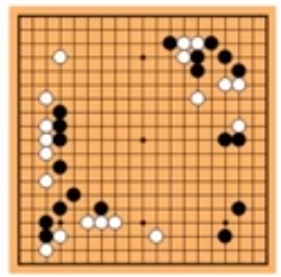Optimization Delayed Consequences Generalization
Supervised ML ad RL		Optimization Generalization
Imitation Learning as RL	Learns from experience…of others; Assumes input demos of good policies Reduces RL to supervised learning	Optimization Delayed Consequences Generalization

Intro to Sequential Decision Making

The problem basically looks like

Goal: Select actions to maximize total expected future reward
May require balancing immediate & long term rewards

Note that it is critical to pick a good reward function. Consider the following RL system:

Agent: AI Teacher
Action: pick a addition or subtraction problem for student to do
World: some student doing the problem
Observation: whether if student did it correctly or not
Reward: +1 if correct, -1 if not

What would happen in this case? The agent could learn to give easy problems.

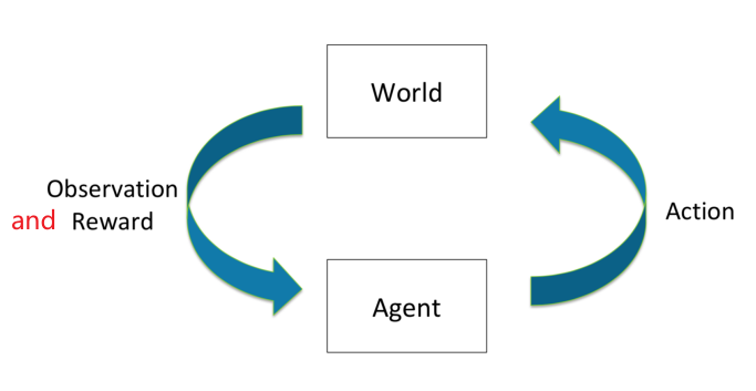
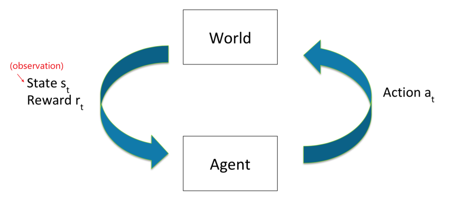
A more formal formulation of the task looks like

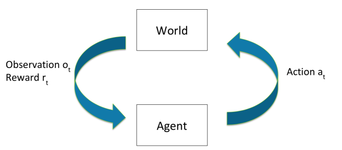
where we have:

at each time $t$
- agent takes some action $a_t$
- world updates given action $a_t$, emits observation $o_t$ and reward $r_t$
- agent receives observation $o_t$ and reward $r_t$
therefore, we essentially have a history $h_t=(a_1,o_1,r_1,…,a_t,o_t,r_t)$
State is information assumed to determine what happens next
- usually the agent uses (some function of) the history to determine what happens next, so $s_t = f(h_t)$
- This is true state of the world is hidden from agent

Markov Assumption and MDP

Why is Markov assumption so popular? It turns out that such an assumption can always be satisfied if we set state as history:

\[p(s_{t+1}|s_t, a_t) = p(s_{t+1}|h_t,a_t)\]

where RHS is like the true model, and LHS is what we are modelling.

However, in practice we often assume the most recent observation being sufficient to model the state

\[p(s_{t+1}|s_t, a_t) = p(s_{t+1}|o_t,a_t)\]

So that:

If we consider most recent observation as your state, so $s_t = o_t$, then the agent is modelling the world as MDP
If agent state is not the same as the world state (e.g. Use history $s_t = h_t$ , or beliefs of world state, or RNN), then it is a Partially Observable MDP, or POMDP
- e.g. playing a poker game, where agent only sees its own card

Or other state representation (e.g. past 4 states). This choice affects how big our state space is, which has big implications for:

Computational complexity
Data required
Resulting performance

An example of this would be:

a state include all history, e.g. our entire life trajectory = have only a single data sample
a state include only most recent life experience = a lot of data samples

Types of Sequential Decision Process

In reality, we may face different types of problems, each with different properties:

Bandits: actions have no influence on next observations
- e.g. whether if I clicked on the advertisement does not affect who the next customer (coming to the website) is
MDP and POMDP: Actions influence future observations
Deterministic World: given the same state and action, we will have the same/only one possible observation and reward
- Common assumption in robotics and controls
Stochastic: given the same state and action, we can have multiple possible observation and reward
- Common assumption for customers, patients, hard to model domains
- can think of the case that we don’t have good enough model for deterministic coin flipping, hence we model it as stochastic

Example of MDP

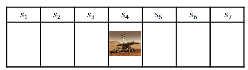
Consider the case of having a Mars Rover exploring, which has seven possible states/locations to explore. We start at state $s_4$

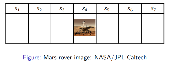
so we have

States: Location of rover $(s_1, …,s_7)$
Actions: Left or Right
Rewards: $+1$ in state $s_1$, $10$ in state $s_7$, $0$ in all other states

We want to find a program that tells the rover what to do next. In general RL problems can be modeled in three ways

Model: Representation of how the world changes in response to agent’s action
- in this case we need to model transition
  \[p(s_{t+1}=s' | s_t = s,a_t=a)\]
  for any action state combination
- and the reward
  \[r(s_t=s,a_t=a) \equiv \mathbb{E}[r_t|s_t =s,a_t=a]\]
  for any action state combination
Policy: function mapping agent’s states to action (i.e. what to do next given current state)
- hence we model, if deterministic
  \[\pi(s)=a\]
  spits out an action given a state
- if stochastic
  \[\pi(a|s) = P(a_t=a|s_t=s)\]
  being a probability distribution given a state.
Value function: Future rewards from being in a state and/or action when following a particular policy
- we consider the expected discounted sum of future rewards under/given a particular policy $\pi$
  \[V_\pi(s_t=s) = \mathbb{E}_\pi [r_t + \gamma r_{t+1} + \gamma^2 r_{t+2}+...|s_t=s]\]
  for $\gamma \in [0,1)$ specifying how much we care about the future reward compared to current reward.

Types of RL Agents

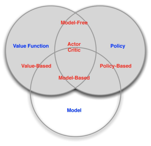
Therefore, from the above discussion, we essentially have two types of RL algorithms:

Model-based
- explicitly having a model of the world (e.g. models the transition function, reward)
- may or may not have an explicit policy and/or value function (e.g. if needed compute from the model)
- no longer needs interaction/additonal experience
Model-free
- explicitly have a value function and/or policy function
- no model of the world

A more complete diagram would be

Key Challenges in Making Decisions

Planning (Agent’s internal computation)
- Given model of how the world works
  - i.e. you already know the transition and rewards
- need an algorithm to compute how to act in order to maximize expected reward
  - With no interaction with real environment
Reinforcement learning (we don’t even have the model)
- Agent doesn’t know how world works
- Interacts with world to implicitly/explicitly learn how world works
- Agent improves policy (may involve planning)

so we see that RL deals with more problems: we also need to decide what action to do for a) getting the necessary information of the world, and b) achieve high future rewards

For instance

Planning: Chess game
- we already know all the possible moves, and rewards (who wins/losses)
- we need an algorithm to tell us what to do next based on this model
  - doing a tree search, etc.
Reinforcement Learning: Chess game with no rule book, i.e. don’t know the rule of chess
- first we need to directly learn by taking actions and see what happens
- Try to find a good policy over time

Important Components in RL

Agent only experiences what happens for the actions it tries. How should an RL agent balance its actions?

Exploration: trying new things that might enable the agent to make better decisions in the future
Exploitation: choosing actions that are expected to yield good reward given past experience

Often there may be an exploration-exploitation tradeoff, as you might not the correct model of the world (since you only have finite experience). May have to sacrifice reward in order to explore & learn about potentially better policy

Another two very important component you often see in RL is:

Evaluation: given some policy, we want to evaluate how good the policy is
Control: find the good policy
- e.g. do policy evaluation, and improve (iff the policy is stochastic)
- so does more than evaluation

MDPs and MRPs

Here we discuss how do we decide to take actions when given a world model. So here we will first discuss the problem of planning, instead of reinforcement learning (discussed later).

Specifically, we will cover

Markov Decision Processes (MDP)
Markov Reward Processes (MRP)
Evaluation and Control in MDPs

Therefore, we basically consider

so mathematically we consider

\[p(s_{t+1}|s_t, a_t) = p(s_{t+1}|o_t, a_t)\]

Markov Process/Chain

Before we discuss MDP, we first consider what is MP.

Markov Process

A Markov process has:

a set of finite states $s \in S$

a dynamics/transition model $P$ that specifies $p(s_{t+1}=s’ \vert s_t=s)$. For a finite number of states, this can be modelled as
\[P = \begin{bmatrix} P(s_1|s_1) & P(s_2|s_1) & \dots & P(s_N|s_1)\\ P(s_1|s_2) & P(s_2|s_2) & \dots & P(s_N|s_2)\\ \vdots & \vdots & \ddots & \vdots\\ P(s_1|s_N) & P(s_2|s_N) & \dots & P(s_N|s_N)\\ \end{bmatrix}\]

notice that we have no action nor rewards: so we basically just observe this process being a memoryless random process

For instance, we can consider Mar’s Rover having the following transition dynamics

Markov World	Transition Model

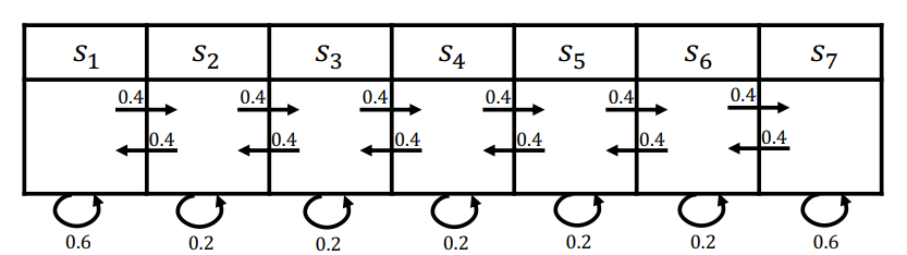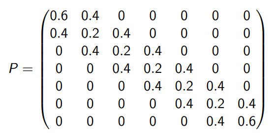where we see that $p(s_1\vert s_1)=0.6$, and $p(s_2\vert s_1)=0.4$, etc.

Using the transition model we can also mathematically compute the probability distribution of the next state given current state. For instance, if we are currently at $s_t=s_1$, then $p(s_{t+1}\vert s_t)$ is modelled by

\[p(s_{t+1}|s_t=s_1) = [1, 0, 0,0,0,0,0]P = \begin{bmatrix} 0.6\\ 0.4\\ 0\\ \vdots\\ 0 \end{bmatrix}\]

Then, a sequence of states you would observe from the world would be sampled from the above distribution, so in the end you only see some deterministic observations/episodes such as

$s_4 \to s_5 \to s_6 \to s_7 \to s_7, …$
$s_4 \to s_5 \to s_4 \to s_5 \to s_7, …$
$s_4 \to s_3 \to s_2 \to s_1 \to s_2, …$
etc.

Markov Reward Process

Markov Reward Process is essentially Markov Chain + Reward

Markov Reward Process:

Markov reward process involves

a set of finite states $s \in S$

a dynamics/transition model $P$ that specifies $p(s_{t+1}=s’ \vert s_t=s)$.

for a finite number of states, this can be expressed as a matrix.

a reward function $R(s_t=s) \equiv \mathbb{E}[r_t \vert s_t=s]$, meaning the reward at a state is the expected reward of that state

for a finite number of states, this can be expressed as a vector.

allow for a discount factor $\gamma \in [0,1]$

mainly for mathematical convenient, which can avoid infinite returns and values/converges

if episodes are finite, then $\gamma = 1$ works

note that we still have no actions.

Once there is a reward, we can consider ideas such as returns and value functions

Horizon: Number of time steps in each episode

Can be infinite

if not, it is called finite Markov reward process

(MRP) Return: discounted sum of rewards from time step $t$ to Horizon
\[G_t = r_t + \gamma r_{t+1} + \gamma^2 r_{t+2} + ...\]
note that

this is like a reward for a particular episode starting from time $t$

why geometric series? This is usually used for its nice mathematical properties.

(MRP) State Value Function $V(s)$: expected return from starting in state $s$
\[V(s) = \mathbb{E}[G_t|s_t=s] = \mathbb{E}[ r_t + \gamma r_{t+1} + \gamma^2 r_{t+2} + ... | s_t=s]\]

note that

if the process is deterministic, then $\mathbb{E}[G_t\vert s_t=s]=G_t$
if the process is stochastic, then it is usually different.

For instance, consider the previous example of

Markov World	Transition Model

but now we have:

$R(s=s_1)=+1$, and $R(s=s_7)=+10$. Zero otherwise

Then consider sampling 2 episodes with 4-step length, using $\gamma=1/2$ we can compute the sample return

$s_4,s_5,s_6,s_7$ having a return of $0+\frac{1}{2}\times 0+\frac{1}{4}\times 0+\frac{1}{8}\times 10=1.25$
$s_4, s_4, s_5, s_4$ having a return of $0+\frac{1}{2}\times 0+\frac{1}{4}\times 0+\frac{1}{8}\times 0=0$

Finally, we can consider the state value function by averaging over all the possible trajectories for each state, and we would get

\[V= [1.53, 0.37, 0.13, 0.22, 0.85, 3.59, 15.31]\]

in this particular example.

How do we compute the state function in reality?

Could estimate by simulation (i.e. generate a large number of episodes and take average)
- notice that this method assumes no Markov process, as we are just sampling and averaging
- we have theoretical bounds as well on how many episodes we need
Or we can utilize the Markov structure and know that MRP value function satisfies
\[V(s) = \underbrace{R(s)}_{\text{imemdiate reward}}+ \quad \underbrace{\gamma \sum_{s'\in S} P(s'|s)V(s')}_{\text{discounted sum of future rewards}}\]

Of course for computation we will use the latter case, which brings us to

Bellman’s Equation for MRP: for fintie state MRP, we can express $V(s)$ for each state using a matrix equation
\[\begin{bmatrix} V(s_1)\\ \vdots\\ V(s_N) \end{bmatrix} = \begin{bmatrix} R(s_1)\\ \vdots\\ R(s_N) \end{bmatrix} + \gamma \begin{bmatrix} P(s_1|s_1) & P(s_2|s_1) & \dots & P(s_N|s_1)\\ P(s_1|s_2) & P(s_2|s_2) & \dots & P(s_N|s_2)\\ \vdots & \vdots & \ddots & \vdots\\ P(s_1|s_N) & P(s_2|s_N) & \dots & P(s_N|s_N)\\ \end{bmatrix}\begin{bmatrix} V(s_1)\\ \vdots\\ V(s_N) \end{bmatrix}\]
or more compactly
\[V = R + \gamma PV\]

Note that both $R, P$ is known. All we need is to solve for $V$. This can be solved in two ways:

directly with liner algebra
iterative using DP

First, solving it with linear algebra

\[\begin{align*} V &= R + \gamma PV\\ V - \gamma PV &= R\\ V &= (I-\gamma P)^{-1}R \end{align*}\]

which requires solving matrix inverses, hence is $\sim O(N^3)$.

Another way to compute $V$ is by dynamic programming:

initialize $V_0(s)=0$ for all state $s$
For $k=1$ until convergence
- for all $s \in S$
\[V_k(s) = R(s) + \gamma \sum_{s' \in S} P(s'|s)V_{k-1}(s')\]

As this is an iterative algorithm, the cost is $O(kN^2)$ for having $k$ iterations (so each iteration updates is only $O(N^2)$)

Markov Decision Process

Finally we add in action as well, so essentially MDPs are Markov Reward Process + actions

Markov Decision Process: MDP involves

a set of finite states $s \in S$

a finite set of actions $a \in A$

a dynamics/transition model $P$ for each action that specifies $p(s_{t+1}=s’ \vert s_t=s, a_t=a)$.

a reward function $R(s_t=s,a_t=a) \equiv \mathbb{E}[r_t \vert s_t=s,a_t=a]$

allow for a discount factor $\gamma \in [0,1]$

note that know we mostly deal with the “joint probability” of $s_t,a_t$ together.

For instance, for the Mars Rover MDP case

World Model	Transition Model

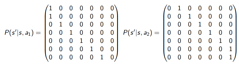where in this case we are having deterministic actions, which nonetheless can be modelled as a stochastic transition with probability of one.

Once we have actions in our model, we also have the following

Policy: specifies what action to take in each state
\[\pi (a|s) = P(a_t=a|s_t=s)\]
Basically a conditional distribution of actions on current state

Note that once you specified a policy, you can convert MDP + policy to a Markov Reward Process, so that

\[R^\pi (s) = \sum_{a \in A} \pi(a|s)R(s,a)\]

is again independent of action in MRP, and similarly

\[P^\pi(s'|s) = \sum_{a\in A}\pi(a|s) P(s'|s,a)\]

which implies we can use same techniques to evaluate the value of a policy for a MDP as we could to compute the value of a MRP

MDP Policy Evaluation

For a deterministic policy $\pi(s)$, we can evaluate the value function $V^\pi(s)$ by, for example, the iterative algorithm mentioned before

initialize $V_0(s)=0$ for all state $s$
For $k=1$ until convergence
- for all $s \in S$
\[V^\pi_k(s) = r(s,\pi(s)) + \gamma \sum_{s' \in S} p(s'|s, \pi(s))V_{k-1}(s')\]
so essentially $V_k^\pi(s)$ is exact value of $k$-horizon value of state $s$ under policy $\pi$, i.e. the value function if we are allowed to act for $k$ steps. Therefore, as $k$ increases we converge to infinite horizon.

This is also called the Bellman backup for a particular (deterministic) policy.

note that of course we could have also computed $V^\pi$ analytically, or with simulation.

For instance, consider the setup of Mars Rover

And in this case we have:

Dynamics: $p(s_6 \vert s_6,a_1)=0.5, p(s_7 \vert s_6,a_1)=0.5, …$
Reward: for all actions, +1 in state $s_1$, and +10 in state $s_7$. Zero otherwise
Policy: $\pi(s)=a_1$ for all states.
$\gamma$ set to $0.5$

Let we initialize with $V^\pi_k=[1,0,0,0,0,0,0,10]$, we want to compute $V^\pi_{k+1}(s_6)$. From the iterative formula

\[\begin{align*} V^\pi_{k+1}(s_6) &= r(s_6, a_1) + \gamma [0.5 * V_k(s_6) + 0.5 * V_k(s_7)]\\ &= 0 + 0.5*[0.5 * 0 + 0.5 * 10]\\ &= 2.5 \end{align*}\]

Notice that we have propagated the reward information from $s_7$ to $s_6$ in this value function! If you do this for all states eventually such an information will be spread in all states.

MDP Control

Ultimately we want our agent to find an optimal policy

\[\pi^*(s) = \arg\max_\pi V^\pi(s)\]

i.e. policy such that its value function is the maximum. Meaning that

A policy $\pi$ is defined to be better than or equal to a policy $\pi’$ if
\[\pi \ge \pi' \iff V_\pi(s) \ge V_{\pi'}(s),\quad \forall s\]
which means its expected return is greater than or equal to that of $\pi’$ for all states. And there is always at least one policy that is better than or equal to all other policies as a policy is essentially a mapping.

Then, it turns out that

Theorem: MDP with infinite horizon:

there exists a unique optimal value function

the optimal policy for a MDP in an infinite horizon problem is

deterministic

stationary: does not depend on time step. (intuition would be that for infinite horizon, you have essentially infinite time/visits for each state, hence the optimal policy does not depend on time)

not necessarily unique

Therefore, it suffices for us to focus on (improving) deterministic policies as our final optimal policy is also deterministic

For example: Consider the Mars Rover case again

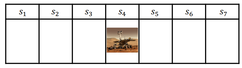
which have 7 states and 2 actions, $a_1, a_2$. How many deterministic policies are there?

since a policy is essentially a mapping from states to actions, there are $2^7$ possible policies.

So how do we search for the best policy?

enumeration: compute for all $\vert A\vert ^{\vert S\vert }$ possible deterministic policy and pick best one
policy iteration: which is more efficient by doing policy evaluation + improvement

MDP Policy Iteration

The goal is to improve a policy iteratively so we end up with an optimal policy:

set $i=0$
initialize $\pi_0(s)$ randomly for all $s$
while $i==0$ or $\vert \vert \pi_i - \pi_{i-1}\vert \vert _1 > 0$ being the L1-norm
1. $V^{\pi_i}$ being the MDP policy evaluation of $\pi_i$
2. $\pi_{i+1}$ being the policy improvement for $\pi_i$ (discuss next)
3. $i = i+1$

How do we improve a policy? First need to consider some new definition

State-Action Value Function: essentially a value function exploring what happens if you take some action $a$ (e.g. different than some given policy) in each state
\[Q^\pi(s,a) = R(s,a)+\gamma \sum_{s' \in S}P(s'|s,a)V^\pi(s')\]
so essentially at each state $s$, we consider:

take action $a$

then follow policy $\pi$

Therefore, using this we can essentially improve a policy $\pi_i$ by:

compute the state-action value of a policy $\pi_i$
- for each state $s\in S$ and $a \in A$
\[Q^{\pi_i}(s,a) = R(s,a) + \gamma \sum_{s' \in S} P(s'|s,a)V^{\pi_i}(s')\]
compute the new policy $\pi_{i+1}$ by
\[\pi_{i+1}(s) = \arg\max_a Q^{\pi_i}(s,a),\quad \forall s\in S\]
to prove that this is a better policy, we need to show that
\[V^{\pi_{i+1}}(s) \ge V^{\pi_i}(s)\]
which we will prove below. (inequality becomes strict if $V^{\pi_i}$ is suboptimal)

Using this approach, we are guaranteed to arrive at the global optimum of best policy.

Proof: Monotonic Improvement in Policy.

We first know that:

\[\max_a Q^{\pi_i}(s,a) \ge V^{\pi_i}(s)=r(s,\pi_i(s)) + \gamma \sum_{s' \in S} p(s'|s, \pi_i(s))V^{\pi_i}(s')\]

by definition of choosing a $\max_a$. Then, notice that

\[\begin{align*} V^{\pi_i}(s) &\le \max_a Q^{\pi_i}(s,a)\\ &= \max_a \{ R(s,a) + \gamma \sum_{s' \in S} P(s'|s,a)V^{\pi_i}(s') \}\\ &= R(s,\pi_{i+1}(s)) + \gamma \sum_{s' \in S} P(s'|s,\pi_{i+1}(s))V^{\pi_i}(s')\\ &\le R(s,\pi_{i+1}(s)) + \gamma \sum_{s' \in S} P(s'|s,\pi_{i+1}(s))\left( \max_{a'} Q^{\pi_i}(s',a') \right)\\\\ &= R(s,\pi_{i+1}(s)) + \gamma \sum_{s' \in S} P(s'|s,\pi_{i+1}(s))\left[ R(s',\pi_{i+1}(s')) + \gamma \sum_{s'' \in S} P(s''|s',\pi_{i+1}(s'))V^{\pi_i}(s'') \right]\\ &\le \dots\\ &= V^{\pi_{i+1}}(s) \end{align*}\]

where:

notice that by definition of $Q^{\pi_{i}}$, we are using $\pi_i$ for future steps on the second and third equality
the third equality comes from the fact that we know $\pi_{i+1}(s) = \arg\max_a Q^{\pi_i}(s,a)$ which spits out the action for maximizing $Q$
the fifth equality is basically doing the same as doing everything from the first to the third equality
hence essentially we are expanding and pushing $\pi_{i+1}$ to a future step, until we are using $\pi_{i+1}$ for all steps

Note that: this is an monotonic improvement

this mean that if the policy didn’t change on one iteration, can it change in future iteration? No, because if taking the max cannot improve it, then it have reached global optimum.

Is there are maximum number of policy iteration? Yes, because there is only $\vert A\vert ^{\vert S\vert }$ number of policies, and since improvement step is monotonic, each policy can only appear once (unless we reached optimal)

MDP Value Iteration

Another approach to find an optimal policy is by value iteration.

policy iteration: for each policy $\pi_i$, we get the value $V^{\pi_i}$ for the infinite horizon and improve it, until obtained best $V^{\pi^*}$
value iteration: maintain the best $V(s)$ up to $k$ number of steps left in the episode, until $k \to \infty$ or converges

so we are computing a different thing here, but the final answer will be the same.

Recall that value of a policy has to satisfy the Bellman equation
\[\begin{align*} V^\pi(s) &= R^\pi(s) + \gamma \sum_{s' \in S} P^\pi(s'|s)V^\pi(s')\\ &=R(s,\pi(s)) + \gamma \sum_{s' \in S} P(s'|s,\pi(s))V^\pi(s') \end{align*}\]
was the definition

Then we can consider a Bellman backup operator which operates on a value function:

\[\mathbb{B}V(s) \equiv \max_a \{ R(s,a) + \gamma \sum_{s'\in S}p(s'|s,a)V(s') \}\]

so basically:

$\mathbb{B}$ is like an operator, which will spit out a new value function
it will improve the value if possible, as this is basically what policy iteration did

Then, with this, we define the algorithm for value iteration:

set $k=1$
Initialize $V_0(s)=0$ for all state $s$
loop until [finite horizon, convergence]
- for each state $s$
  \[V_{k+1}(s) = \max_a \{ R(s,a) + \gamma \sum_{s'\in S}p(s'|s,a)V_k(s') \}\]
  which can be views as just a Bellman backup operation on $V_k$
  \[V_{k+1} = \mathbb{B}V_k\]
then policy for acting $k+1$ steps (best policy) can be easily derived by the action that leads to the best state given current state
\[\pi_{k+1}(s) = \arg\max_a \{ R(s,a) + \gamma \sum_{s'\in S}p(s'|s,a)V_k(s') \}\]
so basically considering best action if only act for $k=1$ step, the use this to compute $k=2$ steps, and etc.

How do we know that this converges? This is because Bellman’s backup operator is a contraction operator (if $\gamma \le 1$)

Difference between Policy and Value iteration

Value iteration

Compute optimal value as if horizon $= k$ steps

Note this can be used to compute optimal policy if horizon $= k$, i.e. finite horizon

Increment $k$

Policy iteration

Compute infinite horizon value of a policy

Use to select another (better) policy

Closely related to a very popular method in RL: policy gradient

Policy Iteration as Bellman Operations

Essentially policy iteration also derives from the Bellman’s constraint, so we can express the policy iteration as Bellman operations as well.

First, we consider Bellman backup operator $\mathbb{B}^\pi$ for a particular policy which operates on some value function (which could have a different policy):

\[\mathbb{B}^\pi V(s) = R^\pi(s) + \gamma \sum_{s'\in S} P^\pi(s'|s)V(s')\]

Therefore, this means that:

policy evaluation of $\pi_i$ is basically doing:
\[V^{\pi_i} = B^{\pi_i}B^{\pi_i}...B^{\pi_i}V\]
for some randomly initialized $V$
policy improvement
\[\pi_{k+1}(s) = \arg\max_a \{ R(s,a) + \gamma \sum_{s'\in S}p(s'|s,a)V^{\pi_k}(s') \}\]

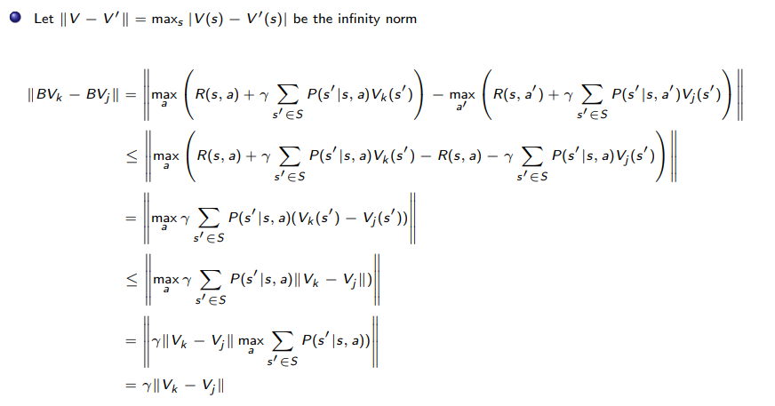
Contraction Operator

Contraction Operator:

Let $O$ be an operator, and $\vert x\vert$ denote any norm of $x$. If
\[|OV-OV'| \le |V-V'|\]
then $O$ is an contraction operator.

so basically

distance between two value functions after applying Bellman’s operator must be less than or equal to distance they had before.
Given this property, it is straightforward to argue that distance between some value function $V$ to the optimal value function $V^*$ will decrease monotonically, hence convergence.

Proof

Policy Evaluation with Unknown World

Before in the MDPs and MRPs section we discussed the problem of planning: if we know how the world works, i.e. have some transition/reward function known, how do we find out the best policy.

However, what if we do not have a world model to begin with? This is what we will discuss in this section, including:

Monte Carlo policy evaluation
Temporal Difference (TD)

Monte Carlo Policy Evaluation

First, recall that with a world model, our algorithm for policy evaluation is:

initialize $V_0(s)=0$ for all state $s$
For $k=1$ until convergence
- for all $s \in S$
\[V^\pi_k(s) = r(s,\pi(s)) + \gamma \sum_{s' \in S} p(s'|s, \pi(s))V_{k-1}(s')\]
so essentially $V_k^\pi(s)$ is exact value of $k$-horizon value of state $s$ under policy $\pi$, i.e. the value function if we are allowed to act for $k$ steps. Therefore, as $k$ increases we converge to infinite horizon.

In other words, we are iteratively estimating $V^\pi(s)$ by $V_k^\pi(s)$ as:

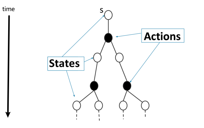
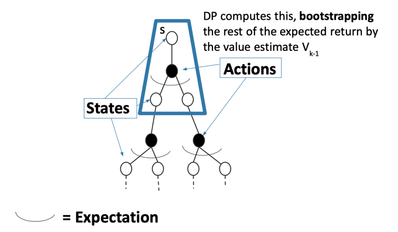
\[V^\pi(s) = \mathbb{E}_\pi[G_t|s_t=s] \approx V_k^\pi(s) = \mathbb{E}_\pi[r_t + \gamma V_{k-1}|s_t=s]\]

we can think update tule graphhically as:

\[V^\pi(s) \leftarrow \mathbb{E}_\pi[r_t + \gamma V_{k-1}|s_t=s]\]

Tree of Possible Trajectories Following a Stochastic $\pi(a\vert s)$	Dynamic Programming Algorithm

where notice that:

essentially we are taking $V_{k-1}^\pi(s)$ for each state as the “true value functions”, and then computing the highlighted expectation by
\[V^\pi(s) \leftarrow r(s,\pi(s)) + \gamma \sum_{s' \in S} p(s'|s, \pi(s))V_{k-1}(s')\]
to update the value functions. Notice that for this to make sense we need to assume infinite horizon, since we are treating $V^\pi(s)$ being stationary for each state, i.e. not a function of time step.
therefore we are bootstrapping as we are taking the value function from previous iteration.
notice that to compute this update we needed $P(s’\vert s,a)$ to average over all possible futures (and $R(s,a)$ as well)

Now, what happens if we do not know the world/model?

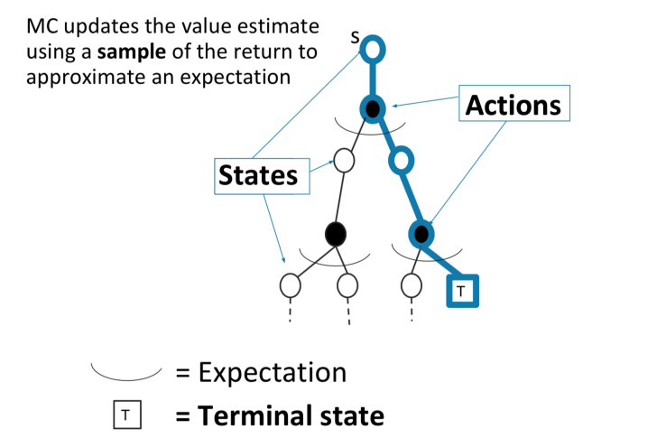
In the framework of MC Policy Evaluation, the idea is to notice that

\[V^\pi(s) = \mathbb{E}_{T \sim \pi}[G_t | s_t=s]\]

basically averaging the $G_t$ of each possible trajectory $T$ following $\pi$, i.e. average over the branches of the tree

therefore, if trajectories are all finite, sample set of trajectories & average returns would give us some approximation of the value function. Hence, properties related to this approach include:

Does not require a known MDP dynamics/rewards, as we just need sample trajectories as its reward
Does not assume state is Markov (e.g. no notion of next state, etc.)
Can only be applied to episodic MDPs
- Requires each episode to terminate

Aim: estimate $V^\pi(s)$ given sampled episodes $(s_1,a_1,r_1,s_2,a_2,r_2,…)$ generated under policy $\pi$

Using this idea of MC policy evaluation, we have the following algorithms that can do this:

first visit MC on Policy Evaluation
every visit MC on Policy Evaluation
incremental MC on Policy Evaluation

First Visit MC On Policy Evaluation

Our aim is to estimate $V^\pi(s)$ by sampling trajectories and taking their mean (as being the MC method). In this case we consider the following algorithm:

Initialize $N(s)=0$, $G(s)=0, \forall s \in S$
loop
1. sample an episode $i=(s_{i,1},a_{i,1},r_{i,1},s_{i,2},a_{i,2},r_{i,2},….,s_{i,T_i})$
2. define $G_{i,t}$ being the return in this $i$-th episode from time $t$ onwards
  \[G_{i,t}=r_{i,t}+\gamma r_{i,t+1} + \gamma^2 r_{i,t+2} + ... + \gamma^{T_i-1} r_{i,T_i}\]
3. for each state $s$ visited in the episode $i$
  1. for the first time $t$ that state $s$ is visited
    1. increment counter of total first visits for that state $N(s)=N(s)+1$
    2. increment total return $G(s)=G(s)+G_{i,t}$
    3. Update estimate $V^\pi(s)=G(s)/N(s)$

How does this algorithm work? How do we know that this way of estimating $V^\pi(s)$ being good (i.e. bias, variance, and consistent)?

Theorem:

$V^\pi$ estimator in this case is an unbiased estimator of the true $\mathbb{E}_\pi[G_t\vert s_t=s]$

$V^\pi$ estimator in this case is also a consistent estimator so that as $N(s)\to \infty$, $V^\pi(s)\to \mathbb{E}_\pi[G_t\vert s_t=s]$

However, those this is a good news, it might not be efficient as we are throwing away many other visits to the same state, which brings us to Every Visit MC On Policy Evaluation

Bias, Variance and MSE Recap

Recall that a way to see if certain estimators work is to compare against the ground truth. Let $\hat{\theta}=f(x)$ be our estimator function (a function of the observed data $x$) for some true parameter $\theta$.

so basically $x \sim P(x\vert \theta)$ being generated from the true parameter
we are constructing an estimator $\hat{\theta}=f(x)$ to estimate such a parameter.
- e.g. for $x \sim N(\mu, \sigma)$, we can estimate $\mu$ by $\hat{\mu} = \text{mean}(x)$ being our estimator

Bias: The bias of an estimator $\hat{\theta}$ is defined by
\[\text{Bias}_\theta(\hat{\theta}) \equiv \mathbb{E}_{x|\theta}[\hat{\theta}] - \theta\]
so that over many sampled datasets, how far is the average $\hat{\theta}$ from the true $\theta$

note that since we don’t know what $\theta$ is in reality, we usually just bound it.

Variance: the variance of an estimator $\hat{\theta}$ is defined by:
\[\text{Var}(\hat{\theta}) \equiv \mathbb{E}_{x|\theta}[(\hat{\theta} - \mathbb{E}[\hat{\theta}])]\]
which is basically the definition of variance itself and has nothing to do with $\theta$

In general different algorithms will have different trade-off between bias and variance.

MSE: Mean squared error of an estimator $\hat{\theta}$ is
\[\text{MSE}_\theta(\hat{\theta}) \equiv \text{Var}(\hat{\theta})+\text{Bias}_\theta(\hat{\theta})^2\]

Every Visit MC On Policy Evaluation

Here, the change is small

Initialize $N(s)=0$, $G(s)=0, \forall s \in S$
loop
1. sample an episode $i=(s_{i,1},a_{i,1},r_{i,1},s_{i,2},a_{i,2},r_{i,2},….,s_{i,T_i})$
2. define $G_{i,t}$ being the return in this $i$-th episode from time $t$ onwards
  \[G_{i,t}=r_{i,t}+\gamma r_{i,t+1} + \gamma^2 r_{i,t+2} + ... + \gamma^{T_i-1} r_{i,T_i}\]
3. for each state $s$ visited in the episode $i$
  1. for the every time $t$ that state $s$ is visited
    1. increment counter of total first visits for that state $N(s)=N(s)+1$
    2. increment total return $G(s)=G(s)+G_{i,t}$
    3. Update estimate $V^\pi(s)=G(s)/N(s)$

Although this is more data efficient as we performed more updates

Theorem:

$V^\pi$ estimator in this case is an biased estimator of the true $\mathbb{E}_\pi[G_t\vert s_t=s]$

the intuition here is that because each state in an episode is not IID, the $G_{i,t}$ is not IID either. Therefore, we will get a biased estimator in this case as we use all encounters of state $s$

$V^\pi$ estimator in this case is a consistent estimator so that as $N(s)\to \infty$, $V^\pi(s)\to \mathbb{E}_\pi[G_t\vert s_t=s]$

Empirically, $V^\pi$ has a lower variance

Incremental MC On Policy Evaluation

In both previous algorithms we had to update the mean incrementally by

first doing $N(s)=N(s)+1$
increment total return $G(s)=G(s)+G_{i,t}$
then update
\[V^\pi(s)=\frac{G(s)}{N(s)}\]

We can also perform the same update incrementally by:

first doing $N(s)=N(s)+1$
update
\[V^\pi(s)=V^\pi(s)\frac{N(s)-1}{N(s)} + \frac{G_{i,t}}{N(s)}=V^\pi(s)+\frac{G_{i,t}-V^\pi(s)}{N(s)}\]
for basically adding a "correction term" of $(G_{i,t}-V^\pi(s))/N(s)$

this idea of a correction term will be used later in TD algorithms, but in practice we can tweak this term so that, if we consider the following algorithm:

Initialize $N(s)=0$, $G(s)=0, \forall s \in S$
loop
1. sample an episode $i=(s_{i,1},a_{i,1},r_{i,1},s_{i,2},a_{i,2},r_{i,2},….,s_{i,T_i})$
2. define $G_{i,t}$ being the return in this $i$-th episode from time $t$ onwards
  \[G_{i,t}=r_{i,t}+\gamma r_{i,t+1} + \gamma^2 r_{i,t+2} + ... + \gamma^{T_i-1} r_{i,T_i}\]
3. for each state $s$ visited in the episode $i$
  1. for the every time $t$ that state $s$ is visited
    1. increment counter of total first visits for that state $N(s)=N(s)+1$
    2. update
      \[V^\pi(s)=V^\pi(s)+\alpha\left( G_{i,t}-V^\pi(s) \right)\]

Then if we used:

$\alpha = 1/N(s)$ then it is the same as every visit MC
$\alpha > 1/N(s)$ then we are placing emphasis on more recent ones/updates $G_{i,t}-V^\pi(s)$.
- this could be helpful if domains are non-stationary. For example in robotics some parts can be breaking down over time, so we want to focus more on more recently learnt data

MC On Policy Example

Consider a simple case of a Mars Rover again:

reward being $R=[1,0,0,0,0,0,0,10]$
initialize $V^\pi(s)=0$ for all $s$
Our policy is $\pi(s)=a_1,\forall s$.
Any action from state $s_1$ or $s_7$ gives termination
take $\gamma = 1$

Suppose then we got a trajectory from this policy:

$T = (s_3,a_1,0,s_2,a_1,0,s_2,a_1,0,s_1,a_1,1,\text)$

Question: What is the first and every visit MC estimate of $V^\pi$?

first visit of $V^\pi(s)=[1,1,1,0,0,0,0]$
every visit is the same even though $s_2$ has two updates

Notice that for all MC methods, we only was able to perform updates until the termination of the episode, since we need to know $G_{i,t}$.

MC On Policy Evaluation Key Limitations

Graphically, what MC algorithms are doing is

Tree of Possible Trajectories Following a Stochastic $\pi(a\vert s)$	MC On Policy Algorithm

So notice that we are averaging across all trajectories, meaning that:

Generally high variance estimator. Reducing variance can require a lot of data
Requires episodic settings (since we can only update once episode terminated)

Temporal Difference Learning

“If one had to identify one idea as central and novel to reinforcement learning, it would undoubtedly be temporal-difference (TD) learning.” – Sutton and Barto 2017

Some key attributes of this algorithm is:

Combination of Monte Carlo & dynamic programming methods
- therefore, it Bootstraps (dynamic programming, reusing $V_{k-1}^\pi(s)$) and samples (MC)
Model-free (does not need to know the transition/reward functions)
Can be used in episodic or infinite-horizon non-episodic settings
Can immediately updates estimate of $V$ after each $(s,a,r,s’)$ tuple, i.e. we do not need to wait until the end-of-episode like MC methods.

Aim: estimate $V^\pi(s)$ given sampled episodes $(s_1,a_1,r_1,s_2,a_2,r_2,…)$ generated under policy $\pi$

this is the same as MC on Policy Evaluation. But recall that if we are having a MDP model, the Bellman Operator can be used to perform an update of the $V(s)$:

\[\mathbb{B}^\pi V(s) = R^\pi(s) + \gamma \sum_{s'\in S} P^\pi(s'|s)V(s')\]

which basically takes the current reward and averages over the value of next state. From this, we consider

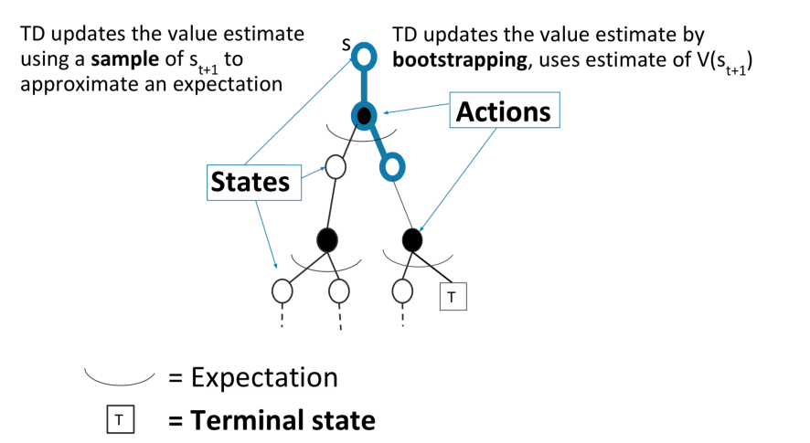
Insight: given some current estimate of $V^\pi$, we can update using
\[V^\pi(s_t) =V^\pi(s_t)+\alpha( \underbrace{[r_t+\gamma V^\pi(s_{t+1})]}_{\text{TD target}}-V^\pi(s_t))\]
for $r_t+\gamma V^\pi(s_{t+1})$ basically is our target (to approximate $r_t+\gamma \sum P^\pi(s’\vert s)V(s’)$) to improve $V^\pi(s)$, as compared to the MC On-policy method which used $G_{i,t}$.

Notice that:

this target is basically also takes the current reward and looks at the value of next state.

we are bootstrapping again, instead of waiting until end of episode, we use previous estimate $V^\pi(s)$ to compute our target $r_t+\gamma V^\pi(s_{t+1})$ and updates at each time step. Therefore we also don’t need episodic requirement.

TD Error: we can also view the above update rule as basically correcting $V^\pi(s)$ by the error term:
\[\delta_t \equiv [r_t+\gamma V^\pi(s_{t+1})]-V^\pi(s_t)\]

Under this framework of TD learning, we also have some variations:

TD(0) Learning: only boostrap
TD($\lambda$) Learning: MC update for $\lambda$ steps and then bootstrap

hence technically we have a continuum of algorithm between using bootstrap and using MC algorithm.

TD(0) Learning

The simplest TD algorithm is TD(0):

input $\alpha$
initialize $V^\pi(s)=0$, $\forall s \in S$
loop
1. sample tuple $(s_t,a_t,r_t,s_{t+1})$
2. update the state:
  \[V^\pi(s_t) =V^\pi(s_t)+\alpha( \underbrace{[r_t+\gamma V^\pi(s_{t+1})]}_{\text{TD target}}-V^\pi(s_t))\]

which is a combination of MC sampling and bootstrapping:

we needed sampling to get $s’$ for evaluating $V^\pi(s_{t+1})$
we used the previous estimate of $V^\pi$ to calculate the values, which is boostrapping

TD(0) Learning Example

Consider a simple case of a Mars Rover again:

reward being $R=[1,0,0,0,0,0,0,10]$
initialize $V^\pi(s)=0$ for all $s$
Our policy is $\pi(s)=a_1,\forall s$.
Any action from state $s_1$ or $s_7$ gives termination
take $\gamma = 1$

Suppose then we got a trajectory from this policy:

$T = (s_3,a_1,0,s_2,a_1,0,s_2,a_1,0,s_1,a_1,1,\text)$

Question: What is the first and every visit MC estimate of $V^\pi$?

first visit of $V^\pi(s)=[1,1,1,0,0,0,0]$
every visit is the same even though $s_2$ has two updates

Question: What is the TD estimate of all states (init at 0, single pass) if we use $\alpha = 1$:

$[1,0,0,0,0,0,0]$. Notice that here we have forgotten the previous history/did not propagate the information of reward at $s_1$ to other states in a single episode.
to propagate this information to $s_2$, we need another episode which had the tuple $s_2 \to s_1$. To propagate to $s_3$, we need yet another episode that contains $s_3 \to s_2$, etc. So this propagation is slow

TD Learning Key Limitations

Graphically, temporal difference considers

MC On Policy Algorithm	TD(0) On Policy Algorithm

so we notice that TD(0):

sits between MC and DP because we are still sampling stuff, but we are updating in a DP fashion

Although this algorithm allows us to update quickly:

it is a biased estimator, since our update rules are using bootstrapping (i.e. $V^\pi(s)$ we used are estimates of the true $V^\pi(s)$, hence it will just be biased)

Comparison Between DP,MC and TD

	DP	MC	TD
Usable when no models of current domain		Yes	Yes
Handles continuing (non-episodic) domains	Yes		Yes
Handles Non-Markovian domains		Yes
Converges to true value in limit (assume Markov)	Yes	Yes	Yes
Unbiased estimate of value	N/A	Yes

note that

for DP, it is the exact estimate.
unbiased = for finite amount of data, on average it is $\theta$; consistent = for infinite amount of data it is $\theta$

Note that here we are still living in the world of tabular state space, i.e. our state space is discrete. Once we move on to the case of having continuous state space, we will cover function approximation methods and a lot of them does not guarantee convergence.

In addition:

MC: updates until end of episode
- Unbiased
- High variance
- Consistent (converges to true) even with function approximation
TD: updates per sample point $(s,a,r,s’)$ immediately
- Some bias
- Lower variance
- TD(0) converges to true value with tabular representation
- TD(0) does not always converge with function approximation

Batch MC and TD

The aim is to use the data more efficiently, hence we might consider:

Batch (Offline) solution for finite dataset:

Given set of $K$ episodes

Repeatedly sample an episode from $K$ (since we are offline, we can replay the episodes)

Apply MC or TD(0) to the sampled episode

The question is, what will MC and TD(0) converge to?

Consider the following example:

Two states $A, B$ with $\gamma = 1$ and a small $\alpha < 1$
Given 8 episodes of experience:
- $A, 0, B, 0$
- $B, 1$ (observed 6 times)
- $B, 0$

Graphically we have

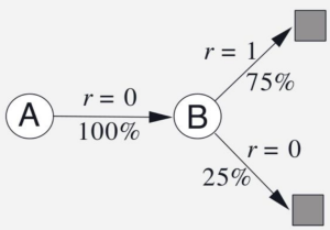
Question: what is $V(A), V(B)$ under MC and TD(0) if we are sampling those data for infinite number of times until convergence?

$V(B)=6/8$ for MC: because in general for 6 out of 8 episodes we get $B\to 1$ in the trajectory
$V(B)=6/8$ for TD(0): because in general 6 out of 8 times we get $B \to \text{Terminate}$ we will have a reward of 1
$V(A)=0$ for MC: in MC setting because updates are done per episode, and the only episode that contained state $A$ had a reward of zero
$V(A)\neq 0$ for TD(0): in TD settings reward propagate back across episodes. Hence once $V(B)\neq 0$ and we sampled a tuple $A\to B$, we will obtain a non-zero value for $V(A)$

Properties of Batch MD and TD

Monte Carlo in batch setting
- converges to min MSE (mean squared error) Minimize loss with respect to observed returns
- MC can be more data efficient than simple TD if markov assumption does not hold (i.e. we need to sample data in TD in order of the episode)
TD(0) in batch setting
- converges to DP policy V π for the MDP with the maximum likelihood model estimates
- TD exploits Markov structure, if it holds then it is very data efficient

Model Free Control

How does an agent learn to act when it does not know how the world works, and does not aim to construct a model (model-free).

Previous section: Policy evaluation with no knowledge of how the world works = how good is a specific policy?
This section: Control (making decisions) without a model of how the world works = how can we learn a good policy?

Many applications can be modeled as a MDP:

Backgammon, Go, Robot locomation, Helicopter flight, Robocup soccer, Autonomous driving, etc.

For many of these and other problems either:

MDP model is unknown but can be sampled
MDP model is known but it is computationally infeasible to use directly, except through sampling (e.g. climate simulation)

Optimization Goal: identify a policy with high expected rewards (without model of the world). Certain features we will encounter like all RL algorithms:

Delayed consequences: May take many time steps to evaluate whether an earlier decision was good or not

Exploration: Necessary to try different actions to learn what actions can lead to high rewards

In this section, we will discuss two types of algorithms:

On-policy Learning
- as we had for policy evaluation
- Direct experience
- Learn to estimate and evaluate a policy from experience obtained from following that policy
Off-policy Learning
- Learn to estimate and evaluate a policy using experience gathered from following a different policy
- e.g. given history $s_1,a_1,s_1,a_1$ and $s_1,a_2,s_1,a_2$, be able to extrapolate what happens if you do $s_1,a_1,s_1,a_2$

MC On-Policy Policy Iteration

Recall that when we know the model, we had the following algorithm for control:

set $i=0$
initialize $\pi_0(s)$ randomly for all $s$
while $i==0$ or $\vert \vert \pi_i - \pi_{i-1}\vert \vert _1 > 0$ being the L1-norm
1. $V^{\pi_i}$ being the MDP policy evaluation of $\pi_i$
2. $\pi_{i+1}$ being the policy improvement for $\pi_i$ (discuss next)
  \[\pi_{i+1}(s) = \arg\max_a \left\{ R(s,a) + \gamma \sum_{s' \in S} P(s'|s,a)V^{\pi_i}(s') \right\} = \arg\max_a Q^{\pi_i}(s,a)\]
which monotonically improves (strict inequality) the policy until optimal policy

Now, we want to do the above two steps without access to the true dynamics and reward models. Notice that essentially policy improvement does $\arg \max_a Q^\pi$, so we want to find a way to estimate $Q^\pi$ directly without knowing world.

previously we have only discussed how to do policy evaluation $V^\pi$ without the world, but not how to improve it

Therefore, we consider the following model-free policy iteration framework:

initialize $\pi_0(s)$ randomly for all $s$
repeat
1. policy evaluation: compute $Q^{\pi_i}(s,a)$
2. policy improvement: update $\pi_{i+1}$ by:
  \[\pi_{i+1} = \arg\max_a Q^{\pi_i}(s,a)\]

But how do we estimate $Q^\pi$?

MC for On Policy Q Evaluation (first visit and every visit)

MC for On Policy Q Evaluation

The idea is basically the same as $V^\pi$ evaluation, where we consider:

Initialize $N(s,a)=0$, $G(s,a)=0, Q^\pi(s,a)=0,\forall s \in S, \forall a \in A$
- in contrast to $V^\pi$ evaluation where we had $N(s)=0, G(s)=0$, etc.
loop
1. sample an episode $i=(s_{i,1},a_{i,1},r_{i,1},s_{i,2},a_{i,2},r_{i,2},….,s_{i,T_i})$
2. define $G_{i,t}$ being the return in this $i$-th episode from time $t$ onwards
  \[G_{i,t}=r_{i,t}+\gamma r_{i,t+1} + \gamma^2 r_{i,t+2} + ... + \gamma^{T_i-1} r_{i,T_i}\]
3. for each state-action pair $(s,a)$ visited in the episode $i$
  1. for the first time or every time $t$ that the pair $(s,a)$ is visited
    1. increment counter of total first visits for that state $N(s,a)=N(s,a)+1$
    2. increment total return $G(s,a)=G(s,a)+G_{i,t}$
    3. Update estimate $Q^\pi(s,a)=G(s,a)/N(s,a)$

Notice that a problem with this algorithm: we can only evaluate $Q^\pi(s,a)$ for state-action pairs that we have experienced. And if $\pi$ is deterministic, we can’t compute $Q^\pi(s,a)$ for any $a\neq \pi(s)$. This means that we cannot say anything about new actions.

The same problem goes with improvement, $\pi_{i+1} = \arg\max_a Q^{\pi_i}(s,a)$ since we have initialized $Q^\pi(s,a)=0,\forall a \in A,\forall s \in S$.

one solution to deal with this is optimistic initialization so we initialize a high $Q^\pi(s,a)$ to promote exploration

This means that our policy improvement will only look at actions we have taken, i.e. it will not explore new state-action pairs so that

\[\pi_{i+1} = \arg\max_a Q^{\pi_i}(s,a)\]

will only end up choosing actions visited by $s,\pi(s)$.

This means we may need to modify the policy evaluation algorithm to include non-deterministic state-action pairs for $Q^\pi(s,a)$

Policy Evaluation with Exploration

Recall that the definition of $Q^\pi(s,a)$ was:

\[Q^\pi(s,a) = R(s,a)+\gamma \sum_{s' \in S}P(s'|s,a)V^\pi(s')\]

so to find a good evaluation of $Q^\pi(s,a)$, we need to:

explore every possible action $a$ from state $s$, to record $R(s,a)$
after that, follow policy $\pi$ to get $\gamma \sum_{s’ \in S}P(s’\vert s,a)V^\pi(s’)$

Insight: since we need to explore every possible action, consider the simple idea to balance exploration and exploitation
\[\pi(a|s) = \begin{cases} \pi(s),& p=1-\epsilon\\ a \in A, & p = \epsilon / |A| \end{cases}\]
which is called the epsilon-greedy policy w.r.t a deterministic policy $\pi(s)$.

This also means we can also define $\epsilon$-greedy policy w.r.t. a state-action value $Q(s,a)$

\[\pi(a|s) = \begin{cases} \arg\max_a Q(s,a),& p=1-\epsilon\\ a \in A, & p = \epsilon / |A| \end{cases}\]

so that you will see we can use this to change the update rule we had, which is $\pi_{i+1} = \arg\max_a Q^{\pi_i}(s,a)$.

For Example: Mars Rovers again, with 7 states:

Now we specify rewards for both actions as we need to compute $Q(s,a)$
\[r(\cdot, a_1) = [1,0,0,0,0,0,10]\\ r(\cdot, a_2) = [0,0,0,0,0,0,5]\]
assume current greedy policy $\pi(s)=a_1$
take $\gamma =1, \epsilon = 0.5$

Then, using $\epsilon$-greedy w.r.t to $\pi(s)$, we got a sampled trajectory of

\[(s_3,a_1,0,s_2,a_2,0,s_3,a_1,0, s_2,a_2,0, s_1,a_1,1, \text{terminal})\]

Question: What is the first visit MC estimate of $Q$ of each $(s,a)$ pair?

$Q^{\epsilon-\pi}(\cdot,a_1)=[1,0,1,0,0,0,0]$ since we are doing MC, we propagates the end-of-episode reward to all states
$Q^{\epsilon-\pi}(\cdot, a_2)=[0,1,0,0,0,0,0]$ same reason as above
notice that without $\epsilon$-greedy, we would have never got $(s_2,a_2,0)$, hence we would have $Q^{\epsilon-\pi}(\cdot, a_2)=[0,0,0,0,0,0,0]$

$\epsilon$-greedy Policy Improvement

Recall that we previous thought of the following as the framework of Model free PI:

set $i=0$
initialize $\pi_0(s)$ randomly for all $s$
while $i==0$ or $\vert \vert \pi_i - \pi_{i-1}\vert \vert _1 > 0$ being the L1-norm
1. $V^{\pi_i}$ being the MDP policy evaluation of $\pi_i$
2. $\pi_{i+1}$ being the policy improvement for $\pi_i$ (discuss next)
  \[\pi_{i+1}(s) = \arg\max_a \left\{ R(s,a) + \gamma \sum_{s' \in S} P(s'|s,a)V^{\pi_i}(s') \right\} = \arg\max_a Q^{\pi_i}(s,a)\]
which monotonically improves (strict inequality) the policy until optimal policy

And we had the problem of $Q^\pi(s,a)$ only containing updates for very small set of $(s,a)$ pairs that we followed a deterministic $\pi(s)$. This means that policy improvement will not try new actions.

Now, the idea is to replace the update step w.r.t the stochastic $\epsilon$-greedy policy $\pi_i$, so that we consider from a $Q^{\pi_i}$ that:
\[\pi_{i+1}(a|s) = \begin{cases} \arg\max_a Q^{\pi_{i}}(s,a),& p=1-\epsilon\\ a \in A, & p = \epsilon / |A| \end{cases}\]
being the new update rule, which now can cover a wider range of $(s,a)$ pairs hence our updated $\pi_{i+1}$ will also contain new actions.

But does this actually provide a monotonic improvement as well (as in the determinstic case)?

Theorem: For any $\epsilon$-greedy policy $\pi_i$, the $\epsilon$-greedy policy $\pi_{i+1}$ w.r.t $Q^{\pi_i}$ is a monotonic improvement, such that $V^{\pi_{i+1}} \ge V^{\pi_i}$

with this theorem, we can have the MC On Policy Improvement/Control algorithm which uses this to provide a better estimate of $Q^\pi(s,a)$ and improve $\pi$

Proof: We just need to show that the value for taking this new policy is higher:

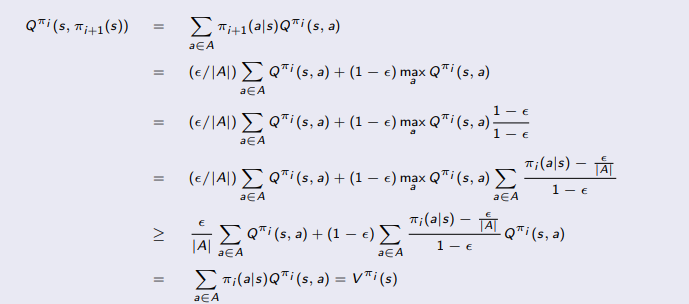
where basically:

on the fourth equality, we utilize the fact that $\sum_{a}\pi_i(a\vert s)=1$
in the last equality, we basically cancelled out the $1-\epsilon$ again and obtained our result
this of course assumes that you know exactly $Q^{\pi_i}$ for a policy $\pi_i$.
- in case when you have an estimate of $Q^{\pi_i}$, then there is no guarantee of monotonic policy improvement. This will happen a lot in function approximation when we have a continuous state space.

This shows that by following $\pi_{i+1}$ the first step and then following $\pi_i$, we get a higher value. Then, we can show $V^{\pi_{i+1}} \ge V^{\pi_i}$ in the similar fashion as we proved the policy improvement by pushing out the $\pi_{i+1}$ policy to future terms.

Finally, we need guarantees on convergence

**GLIE **(Greedy in the Limit of Infinite Exploration):

all state-action pairs are visitied an infintie number of times
\[\lim_{i\to \infty} N_i(s,a) = \infty\]
(satisfied as we have stochastic policy)

Behavior policy (the one we used to sample trajectory) converges to greedy policy (deterministic)
\[\lim_{i \to \infty} \pi(a|s) \to \arg\max Q^\pi(s,a)\]

A practice, instead of having $i \to \infty$, we can also reduce $\epsilon$ to have $\epsilon_i = 1/i$ to also satisfy GLIE (over time we have $0$ prob for exploration).

Theorem: GLIE Monte-Carlo control converges to the optimal state-action value function
\[Q(s,a) \to Q^*(s,a)\]
from which we can find the optimal policy easily by taking $\arg\max_a Q^*(s,a)$

MC On Policy Improvement/Control

Finally, putting everything together, we have the MC On-policy Policy Improvement algorithm as:

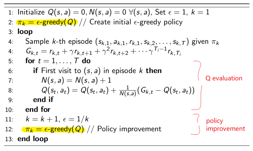
which basically combines:

MC for On Policy Q Evaluation
$\epsilon$-greedy Policy Improvement
and $\epsilon$-Greedy$(Q)$ means that
\[\pi_{k}(a|s) = \begin{cases} \arg\max_a Q(s,a),& p=1-\epsilon\\ a \in A, & p = \epsilon / |A| \end{cases}\]

For Example: Mars Rovers again, with 7 states:

Now we specify rewards for both actions as we need to compute $Q(s,a)$
\[r(\cdot, a_1) = [1,0,0,0,0,0,10]\\ r(\cdot, a_2) = [0,0,0,0,0,0,5]\]
assume current greedy policy $\pi(s)=a_1$
take $\gamma =1, \epsilon = 0.5$

Then, using $\epsilon$-greedy w.r.t to $\pi(s)$, we got a sampled trajectory of

\[(s_3,a_1,0,s_2,a_2,0,s_3,a_1,0, s_2,a_2,0, s_1,a_1,1, \text{terminal})\]

So we know the first visit MC estimate of $Q$ of each $(s,a)$ pair gives:

$Q^{\epsilon-\pi}(\cdot,a_1)=[1,0,1,0,0,0,0]$ since we are doing MC, we propagates the end-of-episode reward to all states
$Q^{\epsilon-\pi}(\cdot, a_2)=[0,1,0,0,0,0,0]$ same reason as above

now, given the policy evaluation:

Question: what is the greedy policy $\pi(s)$ w.r.t this $Q^{\epsilon - \pi}$?

simply $\pi(s) = [a_1,a_2,a_1,\text{tie},\text{tie},\text{tie},\text{tie}]$

Question: therefore, what is the new improved policy $\pi_{k+1}=\epsilon\text{-greedy}(Q)$ if $k=3$?

this means $\epsilon=1/3$
then, from the above result, this means
\[\pi_{k+1}(a|s) = \begin{cases} [a_1,a_2,a_1,\text{tie},\text{tie},\text{tie},\text{tie}], & p=2/3\\ a \in A, & p = 1/6 \end{cases}\]

TD On-Policy Policy Iteration

Recall that the general framework for policy iteration in a model-free case

initialize $\pi_0(a\vert s)$ randomly for all $s$
repeat
1. policy evaluation: compute $Q^{\pi_i}(s,a)$
2. policy improvement: update $\pi_{i+1}$ using $Q^{\pi_i}$

Recall that in the section Policy Evaluation with Unknown World, we had two ways of doing policy evaluation, either doing MC or doing TD. We have come up with a way to compute $Q^\pi(s,a)$ using MC method, therefore, another variant is to use TD method.

Hence, the general algorithm for TD based On-Policy Policy Iteration looks like

initialize $\pi_0(a\vert s)$ randomly for all $s$
repeat
1. policy evaluation using TD: compute $Q^{\pi_i}(s,a)$
2. policy improvement (same as MC): update $\pi_{i+1}$ using $Q^{\pi_i}$ by
  \[\pi_{i+1} = \epsilon\text{-Greedy}(Q^{\pi_i})\]

SARSA

Essentially using TD for policy evaluation:

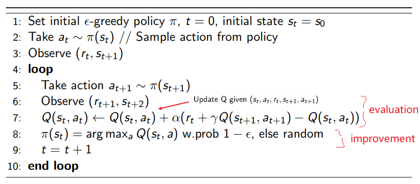
where:

the key change is the update rule
\[Q(s_t,a_t) =Q(s_t,a_t)+\alpha( \underbrace{[r_t+\gamma Q(s_{t+1},a_{t+1})]}_{\text{TD target}}-Q(s_t,a_t))\]
which can perform update per sample instead of waiting until end-of-episode (in MC case).
therefore, notice that the policy are updated much more frequently as well (as compared to the MC case)
the $\alpha$ used is also often called the learning rate in this context

Note that we discarded the notation of $Q^\pi$ here and used $Q$, as we are frequently changing the policy when computing this running estimate to converge to $Q^*(s,a)$

Convergence Properties of SARSA

Theorem: SARSA for finite-state and finite-action MDPs converges to the optimal action-value, $Q(s,a)\to Q^*(s,a)$ ,under the following conditions:

the policy sequence $\pi_t(a\vert s)$ satisfies GLIE

the step size/learning rate $\alpha_t$ satisfy the Robbins-Munro sequence such that
\[\sum_{t=1}^\infty \alpha_t =\infty\\ \sum_{t=1}^\infty \alpha_t^2 < \infty\]
an example would be $\alpha_t = 1/t$

But as the above are conditions sufficient to guarantee convergence, in reality

we could also simply use $\alpha$ being some small constants and empirically they often converge as well
there are also some domains that is hard to satisfy GLIE (e.g. helicopter crashed, can no longer visit some other states). Some research has been working on how to deal with that, but for now we will not worry about it.

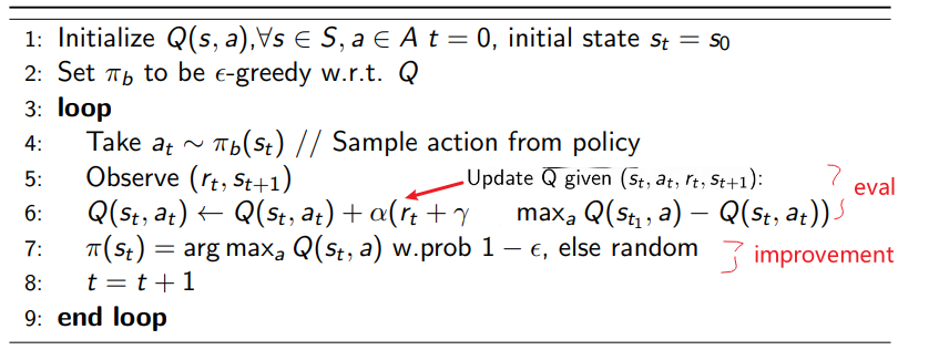
Q-Learning

The only change will be in SARSA

\[Q(s_t,a_t) =Q(s_t,a_t)+\alpha( \underbrace{[r_t+\gamma Q(s_{t+1},a_{t+1})]}_{\text{TD target}}-Q(s_t,a_t))\]

but for Q-learning we consider the update rule:

\[Q(s_t,a_t) =Q(s_t,a_t)+\alpha( \underbrace{[r_t+\gamma \max_{a'} Q(s_{t+1},a')]}_{\text{TD target}}-Q(s_t,a_t))\]

so that

instead of taking $a_{t+1}\sim \pi(a\vert s_{t+1})$, which is being realistic (in SARSA), we are being optimistic so that we update our $Q(s_t,a_t)$ by the best value we could possibly get using $\max_{a’} Q(s_{t+1},a’)$
this means that in cases where we have lots of negative reward/risks in early stages (e.g. cliff walking), SARSA would produce better policy whereas Q-Learning would produce more risky policy

Hence the entire algorithm looks like

where notice that:

we no longer need the $a_{t+1}$ in the five tuple $(s_t, a_t, r_t, s_{t+1}, a_{t+1})$ in SARSA, since we will be taking the next best action
since we are being optimistic, does how Q is initialized matter? Asymptotically no, under mild conditions, but at the beginning, yes
finally, like SARSA it is a policy based on TD, this means that the final reward will only propagate slowly to other states.

Convergence Properties of Q-Learning

What conditions are sufficient to ensure that Q-learning with $\epsilon$-greedy exploration converges to optimal $Q^*$ ?

Visit all $(s, a)$ pairs infinitely often
and the step-sizes αt satisfy the Robbins-Munro sequence.
Note: the algorithm does not have to be greedy in the limit of infinite exploration (GLIE) to satisfy this (could keep $\epsilon$ large).

What conditions are sufficient to ensure that Q-learning with $\epsilon$-greedy exploration converges to optimal $\pi^*$ ?

The algorithm is GLIE (i.e. policy being more and more greedy over time), along with the above requirement to ensure the Q value estimates converge to the optimal Q.

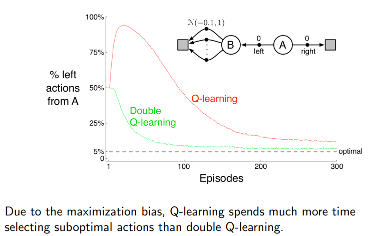
Maximization Bias

Because Q-Learning exploits the greedy action early on, we could have a maximization bias when estimating the value of a policy.

Consider the case of a single state MDP, so that $\vert S\vert =1$, with two actions. And suppose the two actions both have mean random rewards of zero: $\mathbb{E}[r\vert a=a_1]=\mathbb{E}[r\vert a=a_2]=0$

then this means that $Q(s,a_1)=Q(s,a_2)=0=V(s)$ is the true estimate and is optimal.

In practice, we can only do finite samples taking action $a_1,a_2$. Let $\hat{Q}(s,a_1),\hat{Q}(s,a_2)$ be finite sample estimate of $Q$

suppose we used an unbiased estimate of $\hat{Q}(s,a)$ by taking the mean
\[\hat{Q}(s,a_1) = \frac{1}{N(s,a_1)}\sum_{i=1}^{N(s,a_1)}r_i(s,a_1)\]
Let $\hat{\pi}=\arg\max \hat{Q}(s,a)$ be the greedy policy w.r.t the estimated $\hat{Q}$
then we notice that:
\[\begin{align*} \hat{V}^{\hat{\pi}} &=\mathbb{E}[\max (\hat{Q}(s,a_1),\hat{Q}(s,a_2))]\\ &\ge\max(\mathbb{E}[\hat{Q}(s,a_1)],\mathbb{E}[\hat{Q}(s,a_2)]\\ &= \max[0,0]\\ &= V^\pi \end{align*}\]
meaning we have a biased estimator of $V^{\hat{\pi}}$ for the optimal policy.

To solve this, the idea is to instead split samples and use to create two independent unbiased estimates of $Q_1(s_1, a_i)$ and $Q_2(s_1, a_i),\forall a$.

Use one estimate to select max action: $a^* = \arg\max_a Q_1(s_1,a)$
Use other estimate to estimate value of $a^:Q_2(s,a^)$
Yields unbiased estimate: $\mathbb{E}[Q_2(s,a^)]=Q(s,a^)$

This therefore gives birth to the double Q-Learning algorithm

Double Q-Learning

So the only difference is now we have two $Q$ estimates:

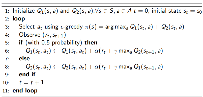
where in practice compared to Q-Learning:

doubles the memory
same computation requirements
data requirements are subtle– might reduce amount of exploration needed due to lower bias

Additionally

Value Function Approximation

In the previous section, we discussed how to do control (make decisions) without a known model of how the world works:

learning a good policy from experience (sampled episodes)
update $Q$ estimate using a tabular representation: finite number of state-action pair

However, as you can imagine many real world problems have enormous state and/or action space so that we cannot really tabulate all possible values. So we need to somehow generalize to those unknown state-actions.

Aim: even if we encounter state-action pairs not met before, we want to make good decisions by past experience.

Value Function Approximation: represent a (state-action/state) value function with a parametrized function instead of a table, so that even if we met an inexperienced state/state-action, we can get some values.

So we imagine

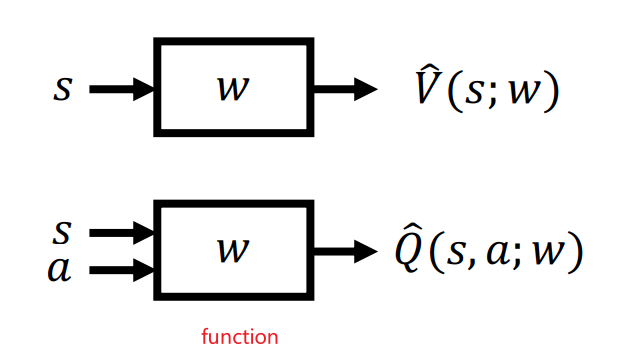
so that essentially we are parameterized the function with weights $W$ as in a deep neural network.

Using such an approach has the following benefits:

Reduce memory needed to store $(P,R)/V/Q/\pi$
Reduce computation needed to compute $(P,R)/V/Q/\pi$
Reduce experience/data needed to find a good $(P,R)/V/Q/\pi$

but this will usually be a tradeoff:

representational capacity (of the DNN to represent states) v.s. memory/computation/data needed

Then most importantly, we need to consider what class of functions do we consider for such an approximation? Many possible function approximators including

Linear combinations of features
Neural networks
Decision trees (useful for being highly interpretable)
Nearest neighbors
Fourier/ wavelet bases

But here we will focus on function approximators that are differentiable, so that we can easily optimize for (e.g. gradient descent). Two popular classes of differentiable function approximators include:

linear feature representations (this section)

neural networks (next section)

Also notice that since we are now doing gradient descent, our approximator will be local optimas instead of the global optimas.

VFA for Policy Evaluation

Aim: find the best approximate representation of $V^\pi$ using a parametrized function $\hat{V}$.

VFA for Policy Evaluation with Oracle

In this case, we consider:

given a policy $\pi$ to evaluate
assume that there is an oracle that returns the true value for $V^\pi(s)$

so we basically want our function approximation to look like the true $V^\pi(s)$ in our space.

Then we can simply perform gradient descent type methods. For instance,

loss function
\[L(w) = \frac{1}{2} \mathbb{E}_\pi[(V^\pi(s) - \hat{V}(s;w))^2]\]
where $\mathbb{E}_\pi$ means expected value over the distribution of states under current policy $\pi$
then gradient update is
\[w:=w - \alpha \left( \nabla_w L(w) \right)\]
and
\[\nabla_w L(w) = \mathbb{E}_\pi[(V^\pi(s)- \hat{V}(s;w))\nabla_w \hat{V}(s)]\]

Then, for instance SGD considers using some batched/single sample to approximate the expected value:

\[\nabla_w L(w) \approx (V^\pi(s)- \hat{V}(s;w))\nabla_w \hat{V}(s)\]

for some sampled $s,V^\pi(s)$.

If we are considering a Linear Value Function Approximation with an Oracle, then simply we consider

\[\hat{V}(s;w) = \vec{x}(s)^T \vec{w}\]

for $\vec{x}(s)$ being a representation of our state. Then we acn also show the gradient to be:

\[\nabla_w L(w) = \mathbb{E}_\pi[(V^\pi(s)- \hat{V}(s;w)) \vec{x}(s)]\]

since $\nabla_w \hat{V} = \vec{x}(s)$ in this case.

Model Free VFA Policy Evaluation

Obviously most of the time we do not have an oracle, which is like knowing the model of the world already.

Aim: do model-free value function approximation for prediction/evaluation/policy evaluation without a model/oracle

recall that this means given a fixed policy $\pi$

estimate its $V^\pi$ or $Q^\pi$

Recall that we have done model-free policy evaluation using tabular methods in:

Monte Carlo Policy Evaluation: update estimate after each episode
Temporal Difference Learning: update estimate after each step

both of which essentially does:

maintain a look up table to store current estimates $V^\pi$ or $Q^\pi$
Updated these estimates after each episode (Monte Carlo methods) or after each step (TD methods)

In VFA, we can basically change the update step to be fitting the function approximation (e.g. gradient descent)

This means that we need to have prepared:

a feature vector to represent a state $s$
\[x(s) = \begin{bmatrix} x_1(s)\\ x_2(s)\\ \dots\\ x_n(s) \end{bmatrix}\]
for instance, for robot navigation, it can be a 180-dimensional vector, with each cell representing the distance to the first detected obstacle. However, notice that this representation also means that it is not markov, as in different hallways (true states) you could have the same feature vector. But it could be still a good representation to condition our decision on.
choose a class of function approximators to approximate the value function
- linear function
- neural networks

MC Value Function Approximation

Recall that for MC methods, we used the following update rule for value function updates

\[V^\pi(s)=V^\pi(s)+\alpha\left( G_{i,t}-V^\pi(s) \right)\]

so that our target is $G_t$, which is an unbiased but noisy estimate of the true value of $V^\pi(s_t)$.

Idea: therere we treat $G_t$ being the “oracle” fo $V^\pi(s_t)$, from which we can get a loss and update our approximator.

This then means our gradient update (for SGD is):

\[\begin{align*} \nabla_w L(w) &=(V^\pi(s_t)- \hat{V}(s_t;w))\nabla_w \hat{V}(s_t)\\ &\approx (G_t- \hat{V}(s_t;w))\nabla_w \hat{V}(s_t) \end{align*}\]

If we are using a linear function:

\[\nabla_w L(w) \approx (G_t- \vec{x}(s_t)^T \vec{w}) \vec{x}(s_t)\]

and then just use $\vec{w} := \vec{w} - \alpha \nabla_w L(w)$ to do descent.

This means that we essentially reduce MC VFA to doing supervised learning on a set of (state,return) pairs: $(s_1, G_1), (s_2, G_2), …, (s_T, G_t)$

Therefore our algorithm with MC updates looks like

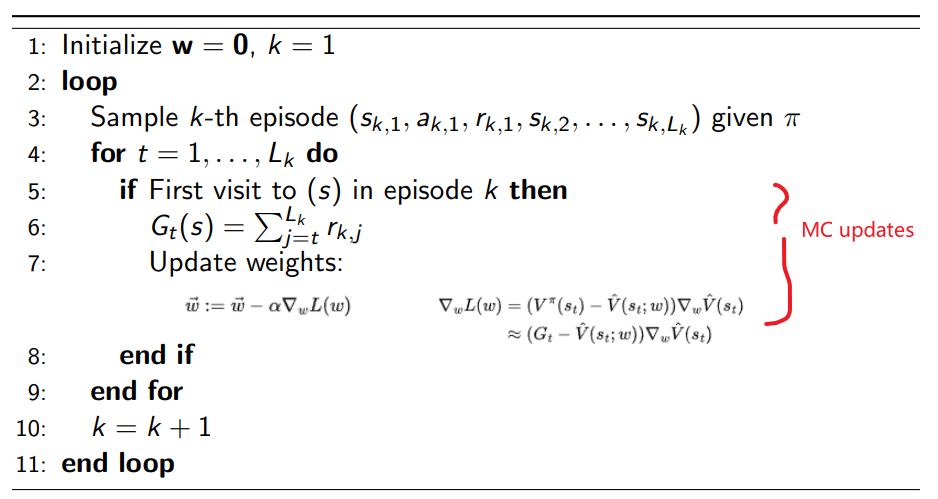
where notice that:

of course you can also have an every-visit version by changing line 5
since we have a finite episode, we used $\gamma=1$ in line 6

For instance: consider a 7 state space with the transition looking like:

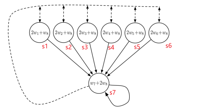
so that:

state $\vec{x}(s_1) = [2,0,0,0,0,0,1]$ so that $\vec{x}(s_1)^T \vec{w} = 2w_1+w_8$, etc.
there are two states, $a_1$ being the solid lines and $a_2$ being the dashed lines.
dashed transition means that here we have a uniform probability $1/6$ to be transitioned to any state $s_i$ for $i \in [1,6]$.
we assume some small termination probability from state $s_7$, but not shown on the diagram
all states have zero reward (so the optimal value function is $V^\pi = 0$)

Suppose we have sampled the following episode:

$s_1, a_1, 0, s_7, a_1, 0, s_7, a_1, 0, \text{terminal}$
we are using a linear function
we have initialized all weights to one $\vec{w}_0 = [1,1,1,1,1,1,1]$
$\alpha = 0.5$, take $\gamma = 1$

Question: what is the MC estimate of $V^\pi(s_1)$? $\vec{w}$ after one update?

first we need $G_1$, which in this case is $0$
our current estimate for $V^\pi(s_1)$ is $\vec{x}(s_1)^T \vec{w}_0 = 2+1=3$
therefore, our update for one step is:
\[\Delta w = -\alpha \cdot (0 - 3) \cdot \vec{x}(s_1) =-1.5\vec{x}(s_1)=[-3,0,0,0,0,0,-1.5]\]
finally, our new weight is therefore $w + \Delta w$:
\[\vec{w}_1 = [-2,1,1,1,1,1,-0.5]\]
so essentially we are doing SGD per state in the episode.

But does such an update converge to the right thing?

Convergence for MC Linear Value Function Approximation

Recall that if provided a policy, then MDP problem is reduced to a Markov Reward Process (by following that policy). Therefore, if we eventually sample many episodes, we get a probability distribution over states $d(s)$, such that:

$d(s)$ is the stationary distribution over states following $\pi$
then obviously $\sum_s d(s) = 1$

Since it is stationary, this means that the distribution after a single transition gives the same $d(s)$:

\[d(s') = \sum_s \sum_a \pi(a|s)p(s'|s,a)d(s)\]

must hold, if the markov process has ran long enough.

Using this distribution, we can consider the mean square error of our estimators for a particular policy $\pi$:

\[MSVE(\vec{w}) = \sum_{s\in S} d(s)\cdot (V^\pi(s) - \hat{V}^\pi(s;\vec{w}))^2\]

for a linear function, we use $\hat{V}^\pi(s;\vec{w}) = \vec{x}(s)^T \vec{w}$.

Theorem: MC policy evaluation with VFA converges to the weights $\vec{w}_{MC}$ which has the minimum mean squared error possible:
\[MSVE(\vec{w}_{MC}) = \min_w \sum_{s\in S} d(s)\cdot (V^\pi(s) - \hat{V}^\pi(s;\vec{w}))^2\]
note that the error might not be zero, e.g. using a linear approximator has only a small capacity.

Batch MC Value Function Approximation

The SGD version basically performs an update per sample, which is suitable for online scenario. However, often we could get a set of episodes already sampled from using a policy $\pi$. Then we can perform a better weight update by considering:

\[\arg\min_\vec{w} \sum_{i=1}^N (G(s_i)- \vec{x}(s_i)^T \vec{w})^2\]

to approximate the expected value version of the MSVE. Then the optimal weights can be solved directly to be:

\[\vec{w} = (X^TX)^{-1} X^T \vec{G}\]

for:

$\vec{G}$ is a vector of all $N$ returns
$X$ is a matrix of the features of each of the $N$ states $\vec{x}(s_i)$
but of course this would be memory intensive as we need to store all $N$ states and returns.
finally, you can obviously have something in between SGD and this full batch.

TD Learning with Value Function Approximation

First recall that TD method considers bootstrapping and sampling to approximate $V^\pi$, so that the update rule is based on per sample:

\[V^\pi(s) = V^\pi(s) + \alpha (r + \gamma V^\pi(s') - V^\pi(s))\]

with the target being $r+\gamma V^\pi(s’)$, which is a biased estimate of the true $V^\pi$.

Idea: use function to represent $V^\pi$, and use boostrapping + sampling in TD method, with the same update rule shown above.

(recall that we are still on-policy, we are evaluating the value of a given policy $\pi$ and all sampled data + estimation are on the same policy)

Therefore, essentially we now consider TD larning being a supervised learning on the set of data pairs:
\[(s_1, r_1 + \hat{V}^\pi(s_2;\vec{w})), (s_2, r_2 + \hat{V}^\pi(s_3;\vec{w})), ...\]
then the MSE loss is simply:
\[L(\vec{w}) = \mathbb{E}_\pi [ (r_j + \gamma \hat{V}^\pi(s_{j+1},\vec{w})) -\hat{V}(s_j; \vec{w})]\]
Hence our gradient step with a SGD update (replacing mean with a single sample) is:
\[\Delta w = \alpha \cdot (r + \hat{V}^\pi(s';\vec{w}) - V^\pi(s;\vec{w})) \cdot \nabla_w \hat{V}^\pi(s;\vec{w})\]
again, with target being $r+\gamma \hat{V}^\pi(s’;\vec{w})$

In the case of a linear function, then we have:

\[\begin{align*} \Delta w &= \alpha \cdot (r + \hat{V}^\pi(s';\vec{w}) - V^\pi(s;\vec{w})) \cdot \nabla_w \hat{V}^\pi(s;\vec{w})\\ &= \alpha \cdot (r + \hat{V}^\pi(s';\vec{w}) - V^\pi(s;\vec{w})) \cdot \vec{x}(s)\\ &= \alpha \cdot (r + \vec{x}(s')^T \vec{w} - \vec{x}(s)^T \vec{w}) \cdot \vec{x}(s)\\ \end{align*}\]

so we are boostrapping our target using our current estimate of $V^\pi(s)$.

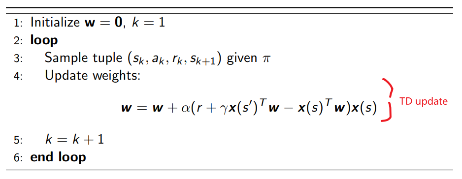
Finally, the algorithm therefore looks like

For instance: we can consider the same example with MC case to compare the difference:

so that:

state $\vec{x}(s_1) = [2,0,0,0,0,0,1]$ so that $\vec{x}(s_1)^T \vec{w} = 2w_1+w_8$, etc.
there are two states, $a_1$ being the solid lines and $a_2$ being the dashed lines.
dashed transition means that here we have a uniform probability $1/6$ to be transitioned to any state $s_i$ for $i \in [1,6]$.
we assume some small termination probability from state $s_7$, but not shown on the diagram
all states have zero reward (so the optimal value function is $V^\pi = 0$)

Suppose we have sampled the following episode:

$s_1, a_1, 0, s_7, a_1, 0, s_7, a_1, 0, \text{terminal}$
we are using a linear function
we have initialized all weights to one $\vec{w}_0 = [1,1,1,1,1,1,1]$
$\alpha = 0.5$, take $\gamma = 0.9$

Question: what is the TD estimate of $V^\pi(s_1)$? $\vec{w}$ after one update of $(s_1,a_1,0,s_7)$?

using the update formula:
\[\Delta \vec{w} = \alpha (0+ 0.9 * 3 - 3)\vec{x}(s_1) = -0.3\alpha \vec{x}(s_1)\]
which is a much smaller weight update than the MC update.

Convergence for TD Linear Value Function Approximation

As mentioned in the MC case, we consider the MSVE for our estimators for a particular policy $\pi$:

\[MSVE(\vec{w}) = \sum_{s\in S} d(s)\cdot (V^\pi(s) - \hat{V}^\pi(s;\vec{w}))^2\]

for a linear function, we use $\hat{V}^\pi(s;\vec{w}) = \vec{x}(s)^T \vec{w}$.

Theorem: TD policy evaluation with VFA converges to the weights $\vec{w}_{TD}$ is within a constant factor of minmum mean squared error possible:
\[MSVE(\vec{w}_{TD}) \le \frac{1}{1-\gamma} \min_w \sum_{s\in S} d(s)\cdot (V^\pi(s) - \hat{V}^\pi(s;\vec{w}))^2\]
so it is slightly worse than MC method as it is biased, but it updates/converges much faster.

As mentioned before, this happens also because we are using

some feature representation for a state which might be a subspace of the true space of states
in TD we are bootstrapping, which gives rise to bias and error

But this also means that if we have some one-hot encoded feature, one for each state, then:

\[\min_w \sum_{s\in S} d(s)\cdot (V^\pi(s) - \hat{V}^\pi(s;\vec{w}))^2 = 0\]

as you can have a unique value per state, even with a linear function. Therefore:

if we used a MC method, then simply:
\[MSVE(\vec{w}_{MC})= \min_w \sum_{s\in S} d(s)\cdot (V^\pi(s) - \hat{V}^\pi(s;\vec{w}))^2 = 0\]
if we used a TD method, then:
\[MSVE(\vec{w}_{TD})\le 0\]
is also optimal, and MC v.s. TD has no difference.

(of course this also means we have enough data)

If our state representation is a subspace of the true state space, then using a TD might incur some error (due to bootstrapping error). But if the state representation is larger or equal to the true state space, then using a TD and MC has no difference.

Control using VFA

Now for control, essentially we consider moving from policy evaluation (previous sections) to policy iteration. This is basically achieved by:

estimate $Q^\pi(s,a)$ instead, using MC or TD technique
perform $\epsilon$-greedy policy improvement

However, this can get unstable because we had the folllowing components:

function approximation (has uncertainty)
bootstrapping (has uncertainty)
off-policy learning for policy improvement (has the biggest uncertainty)
- we are changing the policy over-time, so no longer have a good estimate of the stationary distribution over states of a particular policy

But again, lets first go through the algorithm.

Action-Value Function Approximation with an Oracle

Aim approximate $Q^\pi(s,a)$ given a policy $\pi$, by $\hat{Q}^\pi(s,a)$

The idea is the same as what we see in Model Free VFA Policy Evaluation. Given an oracle $Q^\pi(s,a)$ which spits out the true value, our loss is simply:

\[L(\vec{w}) = \frac{1}{2} \mathbb{E}_\pi [(Q^\pi(s,a) - \hat{Q}^\pi(s,a;\vec{w}))^2]\]

Then for stochastic gradient descent method, the gradient looks like:

\[\begin{align*} \nabla_w L(w) &= \mathbb{E}_w [(Q^\pi(s,a) - \hat{Q}^\pi(s,a;w) ) \nabla_w \hat{Q}^\pi(s,a;w)] \\ &\approx (Q^\pi(s,a) - \hat{Q}^\pi(s,a;w) ) \nabla_w \hat{Q}^\pi(s,a;w) \end{align*}\]

for some sampled $s,a$ pair.

Finally, the features would then should include both a state and action pair:

\[\vec{x}(s,a) = \begin{bmatrix} x_1(s,a)\\ x_2(s,a)\\ \vdots\\ x_n(s,a) \end{bmatrix}\]

For a Linear State Action Value Function Approximation, we consider simply:

\[\hat{Q}(s,a;\vec{w}) = \vec{x}^T(s,a)\vec{w}\]

and the rest is trivial.

Model Free VFA Control

Similar to how we did Model Free VFA Policy Evaluation, the idea is to approximate the oracle with some target.

in MC methods, the target is simply $G_t$, so we consider:
\[\begin{align*} \nabla_w L(w) &\approx (Q^\pi(s,a) - \hat{Q}^\pi(s,a;w) ) \nabla_w \hat{Q}^\pi(s,a;w)\\ &\approx (G_t - \hat{Q}^\pi(s,a;w) ) \nabla_w \hat{Q}^\pi(s,a;w) \end{align*}\]
for SARSA, we used a TD target of $r + \gamma \hat{Q}^\pi(s’,a’;\vec{w})$ which leverages the current function approximation value to bootstrap:
\[\begin{align*} \nabla_w L(w) &\approx (Q^\pi(s,a) - \hat{Q}^\pi(s,a;w) ) \nabla_w \hat{Q}^\pi(s,a;w)\\ &\approx (r + \gamma \hat{Q}^\pi(s',a';\vec{w})- \hat{Q}^\pi(s,a;w) ) \nabla_w \hat{Q}^\pi(s,a;w) \end{align*}\]
and you see for the above update we need $s,a,r,s’,a’$
for Q-Learning, we use the TD target of $r + \gamma \max_{a’}\hat{Q}^\pi(s’,a’;\vec{w})$, which is optimistic and update gradient is:
\[\begin{align*} \nabla_w L(w) &\approx (Q^\pi(s,a) - \hat{Q}^\pi(s,a;w) ) \nabla_w \hat{Q}^\pi(s,a;w)\\ &\approx (r + \gamma \max_{a'}\hat{Q}^\pi(s',a';\vec{w})- \hat{Q}^\pi(s,a;w) ) \nabla_w \hat{Q}^\pi(s,a;w) \end{align*}\]
which we only needs $s,a,r,s’$

For all of the above essentially $\hat{Q}(s,a)$ is a neural network, approximating a function of the feature vectors $\vec{x}(s,a)$

Graphically, the gradient descent algorithms are:

performing a Bellman backup update and
then projecting back to the space of our approximator

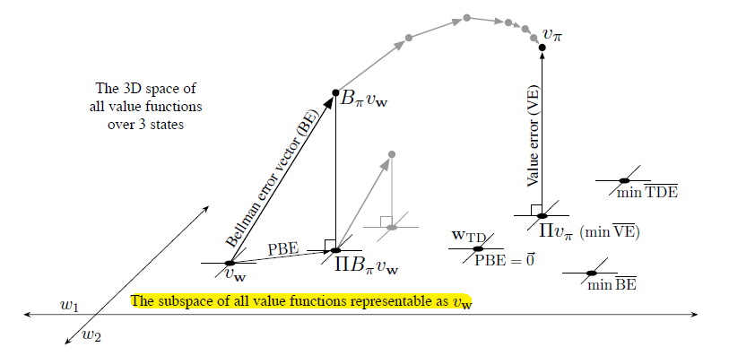
so that we can imagine our control algorithm doing:

the horizontal place is the space of our linear approximator
first we perform one Bellman backup, and reaches $\mathbb{B}^\pi \vec{v}_w$, which is outside of our representation
then, we project back to complete our gradient update $\Pi \mathbb{B}^\pi \vec{v}_w$

However, notice that:

instead of iteratively performing Bellman’s backup outside the space (shown in gray above), which would make us reach the true value function (e.g. dynamic programming), we are constantly projecting back
since we are projecting back at each step, then the final fixed point would be the point of vector-zero PBE
the best approximation $\Pi v_\pi$ in the value error (VE) sense by projecting the true value function, the best approximators in the Bellman error (BE), projected Bellman error (PBE), and temporal difference error (TDE) senses are all potentially different

Convergence of VFA Control

Consider the following example.

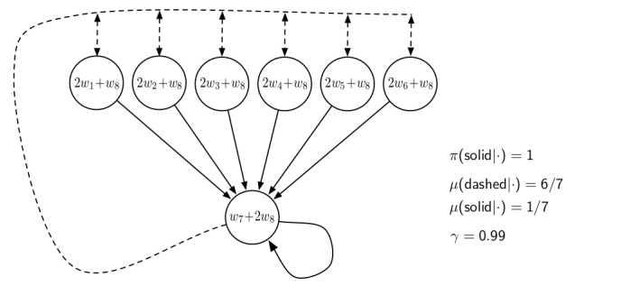
Suppose we want to evaluate the policy of $\pi(\text{solid}\vert \cdot)=1$. Then as we are doing policy iteration, we consider $\epsilon$-greedy policy of:

$\mu(\text{dashed})\vert \cdot)= 6/7$
$\mu(\text{solid})\vert \cdot)= 1/7$
$\gamma = 0.99$

as the behavioral policy used to sample data.

Suppose for simplicity that we then throw away all $(s,a,r,s’)$ tuples whose $a\neq \pi(s)$ which we wanted to evaluate. It turns out that TD-method will diverge:

the stationary distribution of states under the policy we want to approximate will contain a lot of $s_7$ states, so episodes look like $s_1,s_7,s_7,…$
however, the data sampled using our behavior policy will contain episodes such as $s_1,s_7, \text{thrown away}, s_1, s_7, …$

Therefore, the distribution of states we sampled will be very different from the distribution of state under $\pi(s)$.

Hence, in summary:

	Tabular	Linear VFA	Nonlinear VFA
MC Control	Converge	Oscillates but Converge	No guarantee
SARSA	Converge	Oscillates but Converge	No guarantee
Q-Learning	Converge	No guarantee	No guarantee

but as VFA is very important, many research are done on this:

Extensive work in better TD-style algorithms with value function approximation, some with convergence guarantees: see Chp 11 S&B
Exciting recent work on batch RL that can converge with nonlinear VFA (Dai et al. ICML 2018): uses primal dual optimization

Deep Reinforcement Learning

Before, we discussed value function approximation using NN and linear functions. Here, we will focus on RL with function approximation using deep NN:

need to deal with very large state spaces (e.g. for self-driving, video games, etc.)
an intuition for using DNN in RL is to have a DNN to represent the features and the last linear layer represent the linear function approximator for $Q(s,a)$
why is DNN so popular/useful? Universal function approximator theorem.

(the following material assumes you know some basic DNN architectures, including CNNs, RNNs, etc.) Often the idea is to have:

game images as state
game actions as actions (e.g. left, right, up, down, etc.)
game score as rewards
model the $Q$ value function using a DNN

Deep Q Learning

Recall that since Q-Learning was based on TD updates, we had a concern that those off-policy control algorithms can fail to converge:

off-policy control + bootstrapping + function approximation, the deadly triad
we have also seen some simple cases where the such an algorithm does diverge

However, in 2014, DeepMind tried again to combine DNN with RL and achieved extraordinary results in Atari: in practice we can get reasonably good policies out. This is essentially the DQN network:

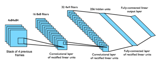
where

since we somehow need to represent velocities in game state, 4-in game frames are taken to represent a state
the network models $Q(s,a)$ for a total of 18 possible joystick actions
reward is the game score

We know that Q-learning with VFA can diverge. Two of the issues are:

correlations between samples: consider an episode of $s,a,r,s’,a’,r’…$. we notice that $V(s)$ would be highly correlated with $V(s’)$ in this case.
non-stationary targets due to bootstrapping: the update target is current approximation, which changes as we perform an update!

DQN addresses those issues by using:

Experience replay: help remove correlations
Fixed Q-targets: help convergence

so that it is more likely to converge.

DQNs: Experience Replay

To help remove correlations, store dataset (called a replay buffer) $D$ from prior experience. So that instead of having updates in the same order as the episode = high correlation, we sample from the buffer.

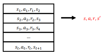
note that this also means we need to decide which experience to put in the buffer.

Usually we can just place the most recent 1 million (for instance) samples in the buffer and sample from it.
this means we also tend to set some fixed probability of how often we will want to sample new experiences

With this, the update step of the algorithm would look like:

sample an experience tuple $(s,a,r,s’) \sim D$ from the replay buffer
compute the target value in a TD fashion as we are doing Q-learning:
\[r + \gamma \max_{a'} \hat{Q}(s',a'| \vec{w})\]
use SGD to update:
\[\Delta w = \alpha (r + \gamma \max_{a'} \hat{Q}(s',a'| \vec{w}) - \hat{Q}(s,a|\vec{w}))\nabla_w \hat{Q}(s,a|\vec{w})\]

now, as mentioned before another problem is that our update target is using the current approximation, which changes as we perform an update. We are chasing a non-stationary target.

DQNs: Fixed Q-Target

To help improve stability, fix the target weights used in the target calculation for multiple updates, instead of having it changed per update.

Let parameters $\vec{w}^-$ and $\vec{w}$ be the weights of the target and current network. Essentially the idea is

sample an experience tuple $(s,a,r,s’) \sim D$ from the replay buffer
compute the target value using $\vec{w}^-$
\[r + \gamma \max_{a'} \hat{Q}(s',a'| \vec{w}^-)\]
use SGD to update:
\[\Delta w = \alpha (r + \gamma \max_{a'} \hat{Q}(s',a'| \vec{w}^-) - \hat{Q}(s,a|\vec{w}))\nabla_w \hat{Q}(s,a|\vec{w})\]
after a certain period, e.g. per 100 steps, update $\vec{w}^- := \vec{w}$.

DQN Ablation Study

How well does the above improve performance?

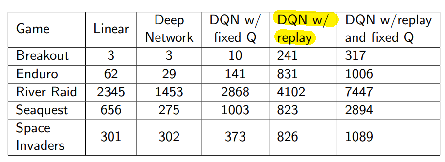
so we see that:

replay is hugely important

DQN Summary

DQN uses experience replay and fixed Q-targets
Store transition $s_t, a_t, r_{t+1}, s_{t+1}$ in replay memory $D$
Sample random mini-batch of transitions $(s,ta,r,s’)$ from $D$
Compute Q-learning targets w.r.t. old, fixed parameters $w^−$
Update using $\epsilon$-greedy exploration, so as before need some decaying exploration
Optimizes MSE loss between Q-network and Q-learning targets

After the success of DQNs, we then had many immediate improvements (many others!)

Double DQN (Deep Reinforcement Learning with Double Q-Learning, Van Hasselt et al, AAAI 2016)
Prioritized Replay (Prioritized Experience Replay, Schaul et al, ICLR 2016)
Dueling DQN (best paper ICML 2016) (Dueling Network Architectures for Deep Reinforcement Learning, Wang et al, ICML 2016)
etc.

Double DQN

Recall that we had Double Q-Learning because we had the maximization bias challenge: Max of the estimated state-action values can be a biased estimate of the max. To solve this issue, there comes the Double Q-learning algorithm which looks like:

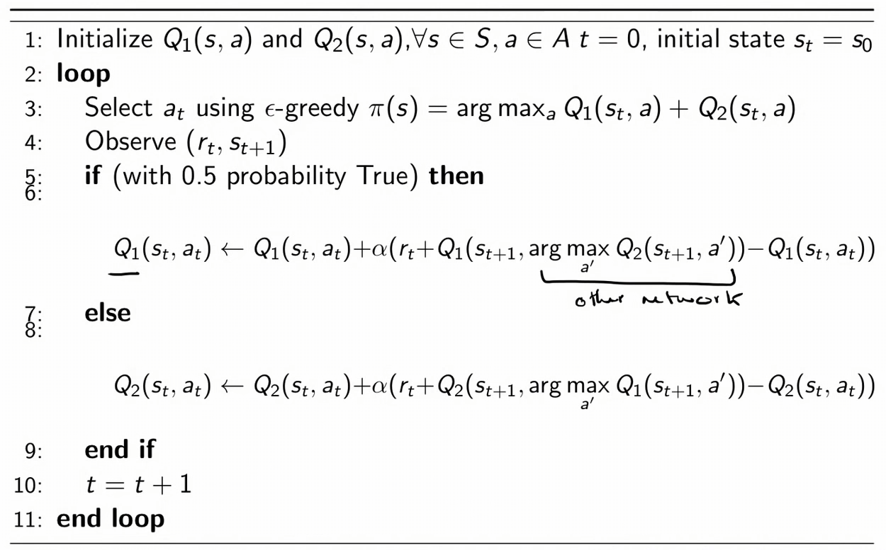
so that we basically maintained two Q-networks.

Extend this idea to DQN using Deep network for the two $Q$ networks.

Result:

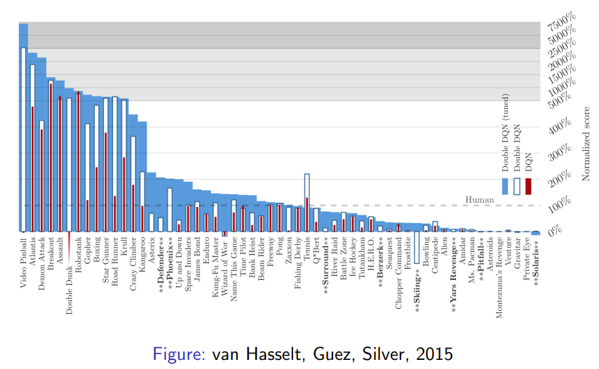
Prioritized Replay

The idea is that instead of sampling randomly from the replay buffer, maybe there are some better distributions to sample such that we can converge better.

Intuitively, consider the following example of the 7-state Mars Rovers again:

reward is $R=[1,0,0,0,0,0,10]$
any action from $s_1,s_7$ are terminal
we initialized with the greedy policy of $\pi(s)=a_1,\forall s$
we sampled a trajectory by having an $\epsilon$-greedy version of the policy $\pi$, and obtained
\[(s_3, a_1, 0,s_2,a_1,0,s_2,a_1,0,s_1,a_1,1,\text{terminal})\]
the TD estimate of all states after an in-order update with $\alpha=1$ is: $[1,0,0,0,0,0,0]$ which we had computed before.
the MC estimate with $\gamma =1$ gives $V = [1,0,0,0,0,0,0]$

Now, using experience buffer, we consider the four tuples:

\[(s_3,a_1,0,s_2), (s_2,a_1,0,s_2), (s_2,a_1,0,s_1), (s_1,a_1,1,T)\]

Question if we get to choose three replay backups to do, which should we pick?

first pick the fourth tuple $(s_1,a_1,1,T)$ so that $V(s_1)=1+\gamma * 0 = 1$
then pick the third tuple $(s_2,a_1,0,s_1)$, because we know that $V(s_1)=1$, so that $V(s_2)= 0 + \gamma * 1$ gets propagated
finally pick the first tuple, $(s_3,a_1,0,s_2)$, because we know that $V(s_2)=\gamma$, and so we can further propagate back to $s_3$.
for $\gamma =1$, this results in $V = [1,0,0,0,0,0,0]$. Notice that it would be the same as MC update!

In theory, such an order is important. There has been research on this and we basically found that if we know the correct order for TD updates, we can require exponentially less updates as sample grows:

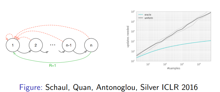
However, computing the exact ordering is intractable in practice.

Therefore, the idea is to consider some ordering based on how big the error is. Consider a sample being $(s_i,a_i,r_i,s_{i+1})$, then we consider the priority of such tuple $i$ being:
\[p_i \equiv \left| \underbrace{r + \gamma \max_{a'}Q(s_{t+1},a';\vec{w}^-)}_{\text{TD target}> }- Q(s_i,a_i;\vec{w}) \right|\]
then the probability of sampling such a tuple is basically proportional to the priority:
\[P(i) \equiv \frac{p_i^\alpha}{\sum_k p_k^\alpha}\]
notice that if we set $\alpha=0$ we get the normal experience replay with equal probability.

Dueling DQN: Advantage Function

The intuition here is that:

Game score may be relevant to predicting $V(s)$
But not necessarily in indicating relative benefit of taking different actions in a state

Therefore, we do not care about the value of a state, but about which actions at state $s$ has a better value, which can be done by looking at the advantage function

\[A^\pi(s,a) \equiv Q^\pi(s,a) - V^\pi(s) = Q^{\pi}(s,a) - Q^{\pi}(s,\pi(s))\]

which is basically the advantage of taking action $a$ at state $s$ compared to taking $\pi(s)$.

Then the architecture looks like:

DQN	Dueling DQN

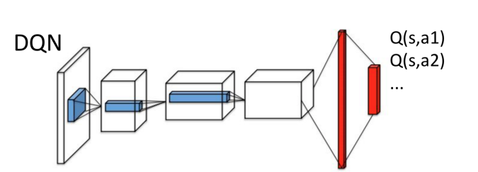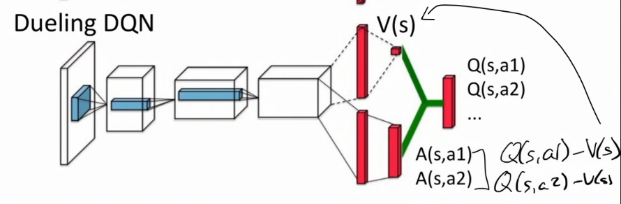where essentially

Dueling DQN keeps one estimate of $V(s)$ from the network and another for the advantage function
then, it is recombined back to $Q(s,a) = A^{\pi}(s,a) - V^{\pi}(s,a)$ to perform the control algorithm.
notice that we are having another set of features to represent $A(s,a)$, which reiterates the point that we might need different features for approximating the advantage than the value function $V\left(s,a\right)$.

When compared to Double DQN with Prioritized Replay, this already has a big improvement:

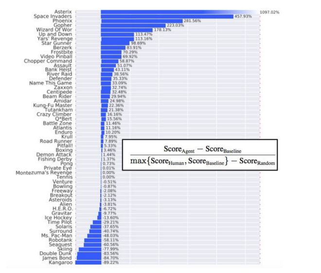
also note that the performance for “Montezuma’s Revenge” was still not improved, i.e. those families of improvements mainly aimed at improving reward propagation, but not for games that require a high exploration.

Identifiability of Advantage Function

However, realize that by the definition of advantage function, this means:

\[\hat{Q}^{\pi}(s,a) = V^{\pi}(s) + A^{\pi}(s,a)\]

but it is not unique as we can have the same $\hat{Q}$ for different $\hat{A}$ and $\hat{V}$. This would be problematic as then our labels for training $A,V$ would be non-unique.

Therefore, the idea is to impose some fixed points:

option 1: Force $A(s,a)=0$ for $a$ is the greedy action
\[\hat{Q}(s,a;\vec{w}) = \hat{V}(s;\vec{w}) + \underbrace{\left( \hat{A}(s,a;\vec{w}) - \max_{a'} \hat{A}(s,a';\vec{w}) \right)}_{\text{approximate } A(s,a)}\]
option 2: Use mean to be zero as the baseline (more stable)
\[\hat{Q}(s,a;\vec{w}) = \hat{V}(s;\vec{w}) + \underbrace{\left( \hat{A}(s,a;\vec{w}) - \frac{1}{\left|\mathcal{A}\right|} \sum\limits_{a'} \hat{A}(s,a';\vec{w}) \right)}_{\text{approximate } A(s,a)}\]

Imitation Learning

Previously we have seen approaches using DNN for learning value functions, and by performing policy iteration, we can improve policy.

However, there exists hardness results that if learning in a generic MDP, can require large number of samples to learn a good policy.

So it is important to remember that:

Reinforcement Learning: Learning policies guided by (often sparse) rewards (e.g. win the game or not):

Good: as a simple, cheap form of supervision

Bad: requires high sample complexity for finding a good policy

Therefore, it most successful when:

in simulation where data is cheap and parallelization is easy

Not when:

Execution of actions is slow
Very expensive or not tolerable to fail (e.g. learning to fly a helicopter will require crashing many times)
Want to be safe

Alternative idea: instead of learning policies from scratch, we could use structure and additional knowledge (if there is) to help constrain and speed reinforcement learning:

imitation learning: we have a fix structure of policy to learn (this section)

policy search/gradient: we have a fixed class of policy to search from (next section)

One application for this is to help improve the performance on “Montezoma’s Revenge” game:

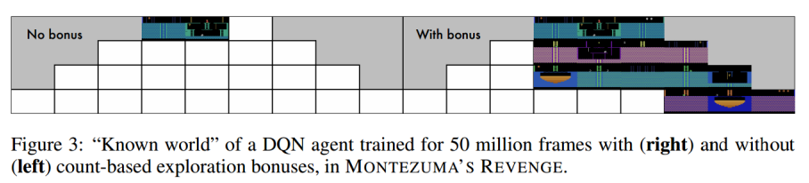
where it is:

a game that you need to collect keys and explore many different rooms
a very very long horizon game, and requires large exploration as well
we see that DQN agents only reached the first two rooms (LHS), with exploration bonus (RHS), we can reach more rooms but still not finishing the game
some of the early approaches to make this work is via imitation learning

Learning from Demonstrations

One of the challenge in Montezuma’s revenge is that long episodes means reward is very sparse. This means that you need to try many different things before getting some feedback of good or bad.

Rewards that are dense in time closely guide the agent:

Manually design them: often brittle

Implicitly specify them through demonstrations: imitation learning!

Therefore, the idea is to have (optimal or pretty good) Expert provides a set of demonstration trajectories: sequences of states and actions

This is useful when it is easier for the expert to demonstrate the desired behavior rather than come up with a reward that would generate such behavior, or coding up the desired policy directly.

Hence in this section, we consider the following problem setup:

given some transition model $P(s’\vert s,a)$
no reward function $R$
given a set of teacher demonstrations $(s_{0,} a_{0}, s_{1,} a_{1} , …)$ drawn from some teacher policy $\pi^{*}$

Aim:

Behavior Cloning: learn the teacher’s policy $\pi^*$

Inverse RL: find the reward function $R$ (e.g. to understand behavior of certain creatures)

Apprenticeship Learning via Inverse RL: find the reward function $R$ and then generate a good policy

Behavior Cloning

The idea of this is simple. Since we need to learn the teacher’s policy $\pi^{*}$, all we need to do is to learn the mapping from state to action.

Therefore, this can be formulated as a supervised machine learning problem:

Fix a policy class (e.g. neural network, decision tree, etc.)

Estimate a policy (i.e. state to action mapping) from training examples $(s_{0} , a_{0}) , (s_{1}, a_{1} ), …$

However, remember that supervised learning assumes iid. $(s, a)$ pairs. This means that

supervised learning assumes the state distribution you will get in any future (e.g. after taking some actions) is the same as the ones in the past (iid)
however, in MDP processes, the state distribution would change after you take some actions.

Problem: Compounding Errors. Therefore errors training in a supervised fashion leads to high generalization error, so that once we went into an unseen state:

assumed same state distribution, hence gets errors

takes the wrong action and continue getting in unseen states

Therefore, we could often get a mismatch in training and test distribution as our data is limited:

train have $s_t \sim D_{\pi^*}$ sampled from the teacher policy

test will encounter $s_t \sim D_{\pi_{\theta}}$ sampled from the our estimated policy

Graphically, this means that as soon as you made a mistake, you will continuously deviate from the path:

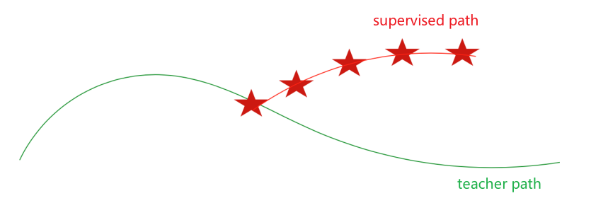
theoretically, the generalization error in this case will be bounded by $\epsilon T^{2}$ instead of $\epsilon T$ bound in supervised learning.

DAGGER: Dataset Aggregation

This is a simple idea to counter the compounding errors problem, so that during training we can ask the expert to provide the gold standard action:

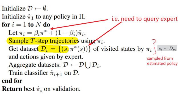
therefore, we get:

in training we have $s_{t} \sim D_{\pi_\theta}$, which will be the same in test environment!
note that we technically don’t need to know the teacher’s policy $\pi^{}$*, we just need to query something to get the gold standard action.

So in this technique we need to have an expert, kind of like human in the loop. Therefore in many cases this could be very label intensive.

Inverse Reinforcement Learning

Recall that our setup was:

given some transition model $P(s’\vert s,a)$
- there are also some extensions on how to do it without transition model as well
no reward function $R$
given a set of teacher demonstrations $(s_{0,} a_{0}, s_{1,} a_{1} , …)$ drawn from some teacher policy $\pi^{*}$

Goal: infer the reward function $R$.

How does this work? Consider the following:

With no assumptions on the optimality of the teacher’s policy, what can be inferred about R?
- nothing, because if the teacher is doing random things, then you have no idea what the reward/goal is.
Now assume that the teacher’s policy is optimal. What can be inferred about R?
- given some optimal path, would the reward function be unique? No: consider the reward function $R=0$ for all states and actions. Then any policy/trajectory would be optimal hence there would be more than one unique answers.
- in fact, a reward function of any constant will have this behavior. Therefore, we need to impose additional constraints to solve this problem

Some of the key papers are:

Maximumum Entropy Inverse Reinforcement Learning (Ziebart et al. AAAI 2008)

Apprenticeship Learning

Recall that the setup is”

given some transition model $P(s’\vert s,a)$
no reward function $R$
given a set of teacher demonstrations $(s_{0,} a_{0}, s_{1,} a_{1} , …)$ drawn from some teacher policy $\pi^*$

Aim: find a policy that is as good as the expert policy

(essentially this comes from trying to solve for the reward function, but realize that it is no longer needed.)

Like linear value function approximation, we can consider a model:

\[R(s) = \vec{w}^{T} \vec{x}(s)\]

for $\vec{x}(s)$ is a feature vector for states.

Then, given a set of demonstrations from $\pi$, we want to identify $\vec{w}$:

\[\begin{align*} V^{\pi} &= \mathbb{E}_\pi\left[\sum\limits_{t=0}^{\infty} \gamma^{t}R(s_t)\right]\\ &= \vec{w}^{T}\mathbb{E}_\pi\left[\sum\limits_{t=0}^{\infty} \gamma^{t}\vec{x}(s_t)\right]\\ &= \vec{w}^{T}\vec{\mu}(\pi) \end{align*}\]

for $\vec{\mu}(\pi) \equiv \mathbb{E}\pi\left[\sum\limits{t=0}^{\infty} \gamma^{t}\vec{x}(s_t)\right]$ can be interpreted as a distribution of states/features weighted by the discount factor.

But we know that an optimal policy will have by definition the largest value function:

\[\begin{align*} V^{*} &\ge V^{\pi}\\ \mathbb{E}_{\pi^{*}}\left[\sum\limits_{t=0}^{\infty} \gamma^{t}R^{*}(s_t)\right] &\ge \mathbb{E}_{\pi}\left[\sum\limits_{t=0}^{\infty} \gamma^{t}R^{*}(s_t)\right]\\ \vec{w}^{*^{T}} \vec{\mu}(\pi^{*}) &\ge \vec{w}^{*^{T}} \vec{\mu}(\pi) \end{align*}\]

From this, the idea is that:

to find the optimal weights $w^{*}$, we need the expert policy to perform better than any other policy (under this reward function)

to perform close to the optimal value $\vec{w}^{*^{T}}$, we just need to match the features under the expert policy

Formally, if

\[||\vec{\mu}(\pi) - \vec{\mu}(\pi^*)||_1 \le \epsilon\]

then for all $\vec{w}$ with $\vert \vert \vec{w}_\infty \vert \vert \le 1$ :

\[||\vec{w}^T\vec{\mu}(\pi) - \vec{w}^{T}\vec{\mu}(\pi^*)||_1 \le \epsilon\]

So that we can find the optimal policy $\pi^{*}$ without needing to know the reward weight $\vec{w}$ by finding a policy $\pi$ such that:
\[||\vec{\mu}(\pi) - \vec{\mu}(\pi^*)||_1 \le \epsilon\]
and for $\vec{\mu}(\pi)$, all we need to know is to compute the discounted sum of features $\vec{x}(s)$ following that policy $\pi$.

Therefore, this gives the Feature Expectation Matching:

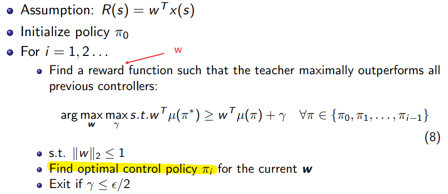
where here we are picking the best policy and picking the corresponding reward function

still doesn’t deal with the problem that reward function is not unique
if expert policy is suboptimal then the resulting policy is a mixture of somewhat arbitrary policies which have expert in the convex hull

Nowadays we tend to use DNN versions, and some extensions include:

GAIL: Generative adversarial imitation learning (Ho and Ermon, NeurIPS 2016)

Imitation Learning Summary

Imitation learning can greatly reduce the amount of data need to learn a good policy
- i.e. think of the expert demonstration as an additional “constraint”/structure
Challenges remain and one exciting area is combining inverse RL / Learning from demonstration and online reinforcement learning

Policy Gradient

Similar to imitation learning, policy gradient/search methods imposes some constraints on the policy and hence makes learning more efficient. However, the changes are:

recall that previously our Policy Improvement algorithm mainly involved:
- policy evaluation: update our estimate of the value function ($V_{\theta} \approx V^{\pi}(s)$ or $Q_{\theta} (s,a) \approx Q^\pi (s,a)$ )
- policy improvement: improve $\pi \gets \epsilon\mathrm{-Greedy}(Q_{\theta} (s,a))$
however, in this section we will directly parametrize the policy, to consider the model:
\[\pi_{\theta} (s,a) \equiv P_\theta[a|s]\]
and the aim is to find a policy $\pi$ with the highest value function $V^{\pi}$.
of course we will do it in a model-free approach (i.e. without transition/reward function)

Graphically, we are at:

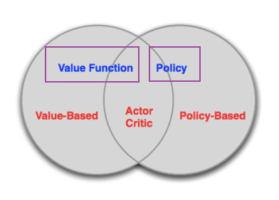
so essentially:

	Learnt/Modelling Value Function	Learnt/Modelling Policy
Value Based (previous sections)	Yes	Implicit (e.g. greedy)
Policy Based (here)	No	Yes
Actor-Critic (next sections)	Yes	Yes

Why might we want to use policy search/gradient methods? Advantages:

Better convergence properties (also depends on computation power)
Effective in high-dimensional or continuous action spaces
Can learn stochastic policies.
- Useful when: exists competitor and do no want to be exploited (e.g. rock-paper-scissor)
- Useful when: the problem is not Markov, e.g. your grey states cannot be distinguished
  
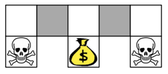
  the problem that states cannot be distinguished is also called aliasing. In this case using stochastic policy in grey states is a good idea/has a higher value.
- Not very useful when: in a tabular MDP problem, optimal policy is deterministic
- monotonic improvement of the policy (value-based methods, e.g. DQN, is noisy)

Disadvantages:

Typically converge to a local rather than global optimum
Evaluating a policy (from which we compute gradient) is typically sample inefficient and high variance

Policy Objective Functions

Goal: given a policy $\pi_{\theta} (s,a)$ parameterized by $\theta$, we want to find $\theta$ that yields the highest value (not value function, but a single score)

in episodic setting (i.e. has terminal states), we can use the start state to compare policies:
\[J_{1}(\theta) = V^{\pi_\theta}(s_1)\]
for $s_1$ is the start state of the entire environment

in continuing/online environment where there is no terminal states, we can use the average value over all states:
\[J_{avV}(\theta) = \sum_s d^{\pi_\theta} (s) V^{\pi_\theta}(s)\]
where $d^{\pi_\theta}(s)$ is the stationary distribution of states for $\pi_\theta$. A similar version of this is to look at the average reward per time-step:
\[J_{avR}(\theta) = \sum_s d^{\pi_\theta}(s) \sum_a \pi_\theta(s,a) R(a,s)\]

Now, we have a goal function from which we can optimize. Therefore, it becomes an optimization problem and we can consider:

gradient free optimization (useful when not differentiable, but not used often now)
- Hill climbing
- Simplex / amoeba / Nelder Mead
- Genetic algorithms
- Cross-Entropy method (CEM)
- Covariance Matrix Adaptation (CMA)
gradient based optimization (this section)
- Gradient descent
- Conjugate gradient
- Quasi-newton

Policy Gradient Methods

Consider the setup of:

Define $V(\theta) \equiv V^{\pi_{\theta}}$ to make explicit the dependence of the value on the policy parameters
assume episodic MDPs

Then policy search/gradient considers gradient ascent w.r.t parameter $\theta$:

\[\nabla \theta = +\alpha \nabla_{\theta} V(\theta)\]

But the question is, what is $\nabla_{\theta} V(\theta)$

\[\nabla_{\theta} V(\theta) = \begin{bmatrix} \frac{\partial V(\theta)}{\partial \theta_1} \\ \frac{\partial V(\theta)}{\partial \theta_2} \\ \vdots\\ \frac{\partial V(\theta)}{\partial \theta_n} \end{bmatrix}\]

when our parameter is on $\pi_\theta$?

Gradients by Finite Differences

The simplest approach to compute this by “trial and error”:

for each dimension $k \in [1, n]$ for $\theta \in \mathbb{R}^{n}$:
1. perturb the parameter by a small amount:
  \[V(\theta + \epsilon u_{k})\]
  for $u_k$ is a unit vector in the $k$-th dimension
2. estimate the gradient w.r.t. $\theta_k$ by:
  \[\frac{\partial V(\theta)}{\partial \theta_k} \approx \frac{V(\theta + \epsilon u_{k}) - V(\theta)}{\epsilon}\]
repeat

While this method seems simple, it has been used practically and was effective (required only few trials).

For instance: AIBO Policy Experiment

The task was to train AIBO robots so that they can walk as fast as possible. Then there was research which had:

open-loop policy: find a sequence of actions, irrespective of the state
12 parameters $\theta \in \mathbb{R}^{12}$ they wanted to search for:
- The front locus (3 parameters: height, x-pos., y-pos.)
- The rear locus (3 parameters)
- Locus length
- Locus skew multiplier in the x-y plane (for turning)
- etc.

Then, essentially they needed to compute the gradient of the policy, which they can by:

Ran on 3 AIBOs at once
Evaluated 15 policies per iteration.
Each policy evaluated 3 times (to reduce noise) and averaged
Used $\eta = 2$ (learning rate for their finite difference approach)

And they were very successful in few iterations:

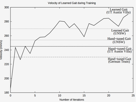
note that as we are converging to local optima, initialization for $\theta$ matters.

Likelihood Ratio/Score Function Policy Gradient

Suppose we can compute $\nabla_{\theta} \pi_\theta(s)$. We want to find a way to compute $\nabla_\theta V(\theta)$ by analytical methods, and one of which is the likelihood ratio policy gradient.

Consider the following setup:

denote a trajectory as $\tau = (s_{0}, a_{0} , r_{0} , … , s_{T-1},a_{T-1},r_{T-1},s_{T},a_{T},r_{T})$.
denote the reward of the trajectory as $R(\tau) \equiv \sum\limits_{t=0}^{T} R(s_t, a_t)$
then define the policy value as:
\[V(\theta) \equiv \sum\limits_{\tau} P_{\pi_\theta}(\tau) R(\tau) = \mathbb{E}_{\pi_{\theta}} \left[ \sum\limits_{t=0}^{T} R(s_{t} , a_{t} ) \right]\]
for $P_{\pi_\theta}(\tau)$ being the probability over trajectories when executing policy $\pi_\theta$.

In this new notation, our goal is to find parameters $\theta$ such that:
\[\arg\max_\theta V(\theta) = \arg\max_\theta \sum\limits_{\tau} P_{\pi_\theta}(\tau) R(\tau)\]
notice that only $P_{\pi_\theta}(\tau)$ changes if you change $\theta$.

Therefore, we are interested in finding $\nabla_\theta V(\theta)$, which can be computed as:

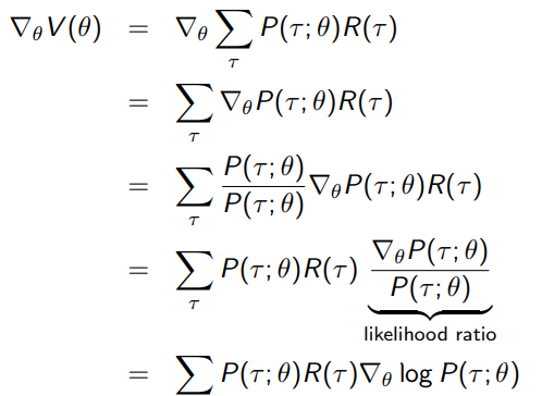
which seems to have done nothing, but we will soon see that

since we are doing model free, this trick helps us to compute $\nabla_\theta \log P(\tau; \theta)$ without knowing the world.
to evaluate $\sum\limits_{\tau}$ and $R(\tau)$, we can just sample a bunch of trajectories!

Therefore, first we approximate this by:

\[\nabla_{\theta} V(\theta) \approx \hat{g} = \frac{1}{m} \sum\limits_{n=1}^{m} R(\tau^{(i)}) \nabla_\theta \log P(\tau^{(i)};\theta)\]

for which $R(\tau^{(i)})$ are known already, and we are weighting each trajectory equally.

The above form of policy gradient can be interpreted as follows: consider the ==generic form of $R(\tau^{(i)}) \nabla_\theta \log P(\tau^{(i)};\theta)$ which can be made into:
\[\hat{g}_i \equiv f(x_i) \nabla_\theta \log p(x_i;\theta)\]
which means that:

$f(x)$ measure how good a sample $x$ is (e.g. $f(x_i) = R(\tau^{(i)})$ )

performing a gradient ascent step means we are pushing up the log probability $p(x_i;\theta)$ of the sample, in proportion to how good it is $f(x)$

note that this form is valid even if $f(x)$ is discontinous

Graphically:

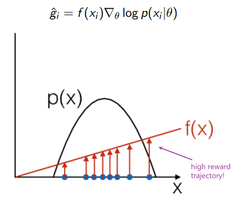
Finally, we need to solve for the term $\nabla_\theta \log P(\tau^{(i)};\theta)$ to compute the gradient $\nabla_{\theta} V(\theta) \approx \hat{g}$:

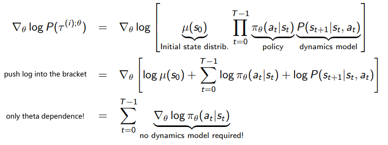
notice that from this we only need to know $\nabla_{\theta} \log \pi_\theta$! This term also gets a (relatively useless) name of score function.

Score Function Policy Gradient:

The goal is to find $\theta$ such that:
\[\arg\max_\theta V(\theta) = \arg\max_\theta \sum\limits_{\tau} P_{\pi_\theta}(\tau) R(\tau)\]
which we can find local optimal using gradient ascent, by:
\[\begin{align*} \nabla_{\theta} V(\theta) \approx \hat{g} &= \frac{1}{m} \sum\limits_{n=1}^{m} R(\tau^{(i)}) \nabla_\theta \log P(\tau^{(i)};\theta)\\ &= \frac{1}{m} \sum\limits_{n=1}^{m} R(\tau^{(i)}) \sum_{t=0}^{T-1} \nabla_\theta \log \pi_\theta(a_t^{(i)}|s_t^{(i)}) \end{align*}\]
and the $m$ trajectories would be sampled under policy $\pi_\theta$. Notice that this is model free as we only need to evaluate the score function $\nabla_{\theta} \log \pi_\theta$.

Finally, it turns out that this can be extended to many other objective functions $J$ than the one shown above $J = V(\theta) = \sum\limits_{\tau} P_{\pi_\theta}(\tau) R(\tau)$.

Policy Gradient Theorem: for any differentiable policy $\pi_{\theta} (s,a)$, for any policy objective function:

episodic $J = J_1$

average reward per time step $J = J_{avR}$

average value $J = (1 / (1 - \gamma)) J_{avV}$ the policy gradient is:

\[\nabla_\theta J(\theta) = \mathbb{E}_{\pi_\theta} [ Q^{\pi_\theta}(s,a) * \nabla_{\theta} \log \pi_\theta (a|s) ]\]
which can be derived in the same manner as we have shown here (also shown in Sutton and Barto chapter 13)

Reducing Variance in Policy Gradient

Previously, we were able to compute policy gradient without a world model by:

\[\nabla_{\theta} V(\theta) \approx \frac{1}{m} \sum\limits_{n=1}^{m} R(\tau^{(i)}) \sum_{t=0}^{T-1} \nabla_\theta \log \pi_\theta(a_t^{(i)}|s_t^{(i)})\]

for letting the objective function being $J = V(\theta)$. However, although this is an unbiased estimate of the gradient, it is noisy (high variance) in practice. Fixes include:

temporal structure/bootstrapping methods (reduces variance)
baseline
alternatives to using MC return $R(\tau^{(i)})$ as targets, e.g. Actor-Critic methods for TD and bootstrapping

Policy Gradient: Use Temporal Structure

It turns out that we can manipulate the same expression we had to achieve another gradient expression. Consider the previous conclusion:

\[\nabla_{\theta} \mathbb{E}_\tau [R] = \mathbb{E}_\tau \left[ R \left( \sum\limits_{t=0}^{T-1} \nabla_\theta \log \pi_\theta(a_t|s_t) \right) \right]\]

for $R = \left( \sum\limits_{t=0}^{T-1} r_t \right)$. This means that:

\[\nabla_{\theta} \mathbb{E}_\tau [r_{t'}] = \mathbb{E}_\tau \left[ r_{t'} \left( \sum\limits_{t=0}^{t'} \nabla_\theta \log \pi_\theta(a_t|s_t) \right) \right]\]

Hence we can recover the original form by summing over $t$:

\[\begin{align*} \nabla_{\theta} V(\theta) = \nabla_{\theta} \mathbb{E}_\tau [R] &= \mathbb{E}_\tau \left[ \sum\limits_{t'=0}^{T-1} r_{t'} \sum\limits_{t=0}^{t'} \nabla_\theta \log \pi_\theta(a_t|s_t) \right] \\ &= \mathbb{E}_\tau \left[ \sum\limits_{t=0}^{T-1} \nabla_\theta \log \pi_\theta(a_t|s_t) \sum\limits_{t'=t}^{T-1} r_{t'} \right] \\ &= \mathbb{E}_\tau \left[ \sum\limits_{t=0}^{T-1} \nabla_\theta \log \pi_\theta(a_t|s_t) G_{t'} \right] \end{align*}\]

where

the second last equality is due to the fact that, the $\nabla_\theta \log \pi_\theta(a_0\vert s_0)$ appears for all $r_{t’}$, and the $\nabla_\theta \log \pi_\theta(a_1\vert s_1)$ appears for all except $r_{t’ = 0}$, etc.
the last equality is due to the fact that $G_{t’}$ is the expected return since time $t’$

Therefore, this yields a slight lower variance estimate of the gradient:
\[\nabla_{\theta} V(\theta) = \nabla_\theta \mathbb{E}_\tau [R] \approx \frac{1}{m} \sum_{i=1}^m \sum_{t=0}^{T-1} \nabla_\theta \log \pi_\theta(a_t^{(i)}|s_t^{(i)}) G_t^{(i)}\]

Notice that

as compared to the previous form $\nabla_{\theta} V(\theta) \approx \frac{1}{m} \sum\limits_{n=1}^{m} R(\tau^{(i)}) \sum_{t=0}^{T-1} \nabla_\theta \log \pi_\theta(a_t^{(i)}\vert s_t^{(i)})$, we multiply each $\nabla_\theta \log \pi_\theta(a_t^{(i)}\vert s_t^{(i)})$ by its own expected reward $G_t^{(i)}$ instead of the constant episodic reward $R(\tau^{(u)})$. This reduces the variance of the gradient estimate.
since this uses $G_t$, it is a MC estimate.

REINFORCE Algorithm

If we sample only one trajectory (doing SGD), then essentially the previous section says:

\[\nabla_{\theta} V(\theta) \approx \sum_{t=0}^{T-1} \nabla_\theta \log \pi_\theta(a_t^{(i)}|s_t^{(i)}) G_t^{(i)}\]

for an sampled trajectory $i$. And this is basically what REINFORCE algorithm does:

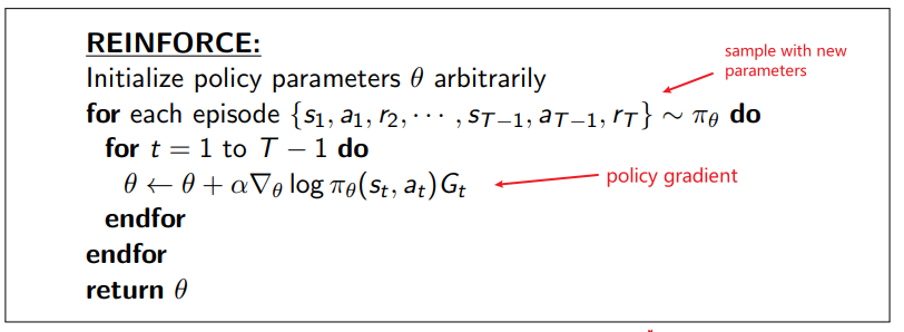
and of course if $\pi_{\theta} (a\vert s)$ is a neural network, then derivative can easily numerically evaluated as well (e.g. automatic differentiation in PyTorch/Tensorflow).

Differentiable Policy Classes

Besides neural network, there are two classes of policy model that can be good to know:

Softmax Policy: weight action using linear combination of feature $\phi(s,a)$ so that:
\[\pi_\theta(a|s) = \mathrm{Softmax}\left( \phi(s,a)^{T} \theta \right)\]
which outputs a probability per discrete action. The score function for this type of model is:
\[\nabla_{\theta} \log \pi_{\theta} (a|s) = \phi(s,a) - \mathbb{E}_{\pi_{\theta}} [\phi(s, \cdot )]\]
Gaussian Policy: very useful for continuos action space, which we can parametrize by:
\[\pi_\theta(a|s) \sim N( \mu(s), \sigma^{2})\]
for variance can be a fixed constant or parametrized as well. We model the mean by:
\[\mu(s) = \phi(s)^{T} \theta\]
being a linear combination again. Then the score function for this is:
\[\nabla_{\theta} \log \pi_{\theta} (a|s) = \frac{(a- \mu(s))\phi(s)}{\sigma^{2}}\]

Policy Gradient: Introduce Baseline

Another way to improve gradient estimates is to use a baseline $b(s_t)$. In the previous section we have derived:

\[\nabla_{\theta} V(\theta) = \nabla_{\theta} \mathbb{E}_\tau [R] = \mathbb{E}_\tau \left[ \sum\limits_{t=0}^{T-1} \nabla_\theta \log \pi_\theta(a_t|s_t) \sum\limits_{t'=t}^{T-1} r_{t'} \right]\]

It turns out that we can reduce variance by:

\[\nabla_{\theta} V(\theta) = \nabla_{\theta} \mathbb{E}_\tau [R] = \mathbb{E}_\tau \left[ \sum\limits_{t=0}^{T-1} \nabla_\theta \log \pi_\theta(a_t|s_t) \left( \sum\limits_{t'=t}^{T-1} r_{t'} - b(s_t) \right)\right]\]

which is still an unbiased estimate:

a near optimal choice is to consider $b(s_t)$ as the expected return $b(s_{t}) \approx \mathbb{E}[r_{t} + r_{t+1} + … + r_{T-1}]$.
in that case, this means that we are increasing logprob of action at proportionally to how much returns $\sum\limits_{t’=t}^{T-1} r_{t’}$ are better than expected.

Why does this not introduce bias? We can prove this by showing:

\[\mathbb{E}_\tau \left[ \nabla_\theta \log \pi_\theta(a_t|s_t) b(s_t) \right] = 0\]

Proof:

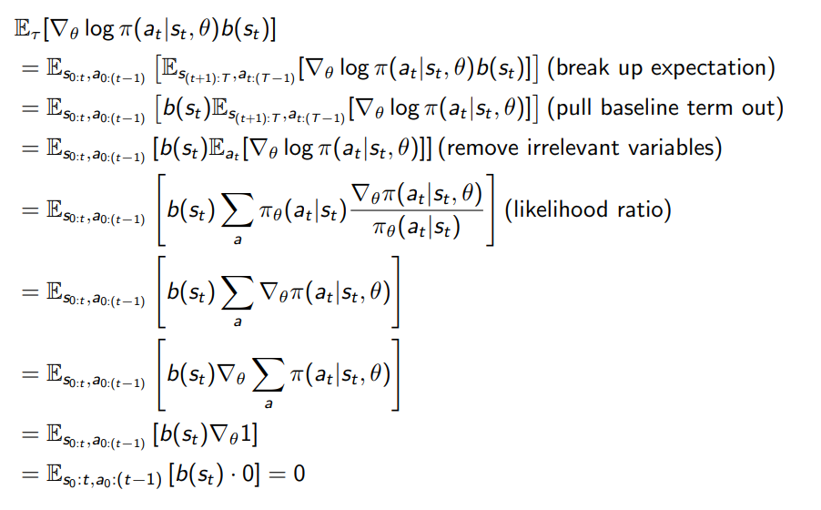
note that this holds for any $b(s_t)$ that is a function of states, and:

the second equality holds because $b(s_t)$ only depends on current and past states
the fourth equality holds because the probability of getting an action $a_t$ given $s_t$ is exactly specified by $\pi_{\theta} (a_{t} \vert s_t)$

Finally the question is what choice of $b(s_t)$ could reduce variance? There will be a number of choices, and some of which we will discuss next.

Vanilla Policy Gradient Algorithm and Auto Differentiation

Using the baseline $b(s_t)$ derivation, the simplest algorithm would look like:

initialize policy parameter $\theta$, baseline $b$ (e.g. a NN, or a lookup table)
for iteration $i=1,2, …$:
1. collect a set of trajectory using current policy $\pi_\theta$:
2. (MC target) at each time step $t=1 , … , \vert \tau^{(i)}\vert$:
  1. compute average return $G_t^{(i)} = \sum_{t’=t}^{T}r_t^{(i)}$
  2. compute advantage estimate: $A_t^{(i)} = G_t^{(i)} - b(s_t)$
3. refit the baseline by minimizing $\sum\limits_{i} \sum\limits_{t} \left\vert b(s_t^{(i)}) - G_t^{(i)} \right\vert ^{2}$
  - or instead of going over all trajectories (off-policy), we can only use the trajectories of the most recent iteration as well (on-policy)
  - if only current iteration is used, then baseline is basically estimating $b(s_{t}) \approx V^{\pi_\theta}$ of the current policy
4. (Policy Improvement) update the policy by policy gradient estimate by summing:
  \[\nabla_\theta \log \pi_\theta(a_t|s_t) \hat{A}_t\]
  and plug this into SGD or ADAM, etc.

Practically, many libraries have auto differentiation. Therefore, instead of calculating manually:
\[\nabla_\theta \log \pi_\theta(a_t|s_t) \hat{A}_t\]
we can just define a surrogate loss function:
\[L(\theta) \equiv \sum_t \log \pi_\theta(a_t|s_t) \hat{A}_t\]
And then let auto differentiation compute the gradient:
\[\hat{g} = \nabla_\theta L(\theta)\]

Policy Gradient: Actor-Critic Methods

In the previous algorithm, we used MC targets which derives from the form:

\[\nabla_{\theta} V(\theta) \approx \frac{1}{m} \sum\limits_{n=1}^{m} R(\tau^{(i)}) \sum_{t=0}^{T-1} \nabla_\theta \log \pi_\theta(a_t^{(i)}|s_t^{(i)})\]

having $R(\tau^{(i)})$ as a target we know leads to high variance but is unbiased (MC updates). But we can then reduce variance by introducing bias using bootstrapping and function approximation (e.g. TD vs MC)

Actor-Critic Methods: Estimate the value function $V$ or $Q$, called critic. Therefore, it maintains an explicit representation of both the policy and the value function, and update both. (e.g. A3C model)

Therefore, in the actor-critic case, we consider instead of:

Use:

\[\nabla_{\theta} V(\theta) = \nabla_{\theta} \mathbb{E}_\tau [R] = \mathbb{E}_\tau \left[ \sum\limits_{t=0}^{T-1} \nabla_\theta \log \pi_\theta(a_t|s_t) \left( Q(s_t,a_t;w)- b(s_t) \right)\right]\]

for $Q(s_t,a_t;w)$ being another function approximator using weights $w$. If we choose $b(s_t)$ to be the value function, then this becomes

\[\nabla_{\theta} V(\theta) = \mathbb{E}_\tau \left[ \sum\limits_{t=0}^{T-1} \nabla_\theta \log \pi_\theta(a_t|s_t) \hat{A}^{\pi} (s_{t}, a_t) \right], \quad \hat{A}^{\pi} (s_{t}, a_{t}) \equiv Q(s_{t}, a_{t} ) - V(s_t)\]

N-step Estimators

It turns out that how exactly we model the $Q$ function can also be varied. Recall that

\[\nabla_{\theta} V(\theta) \approx \frac{1}{m} \sum\limits_{n=1}^{m} R(\tau^{(i)}) \sum_{t=0}^{T-1} \nabla_\theta \log \pi_\theta(a_t^{(i)}|s_t^{(i)})\]

The critic can select any blend between TD and MC estimates for the true-state action value function:

$\hat{R}t^{(1)} = r{t} + \gamma V(s_{t+1})$ being “TD(0)”, for which you bootstrap the value $V(s_{t+1})$ from your critic
$\hat{R}t^{(2)} = r{t} + \gamma r_{t+1} + \gamma^{2} V(s_{t+2})$ being “TD(1)”
…
$\hat{R}t^{(\infty)} = r{t} + \gamma r_{t+1} + \gamma^{2}r_{t+2} + … = G_t$ being MC

From this , ths means hhat the critic can model $V$ and choose between:

$\hat{A}t^{(1)} = r{t} + \gamma V(s_{t+1}) - V(s_t)$
$\hat{A}t^{(2)} = r{t} + \gamma r_{t+1} + \gamma^{2} V(s_{t+1}) - V(s_t)$
…
$\hat{A}t^{(\infty)} = r{t} + \gamma r_{t+1} + \gamma^{2} r_{t+2} + … - V(s_{t}) = G_{t} - V(s_t)$ becomes the MC update used in the (Vanilla Policy Gradient Algorithm)[#Vanilla Policy Gradient Algorithm and Auto Differentiation].

to plug into the gradient equation:

\[\nabla_{\theta} V(\theta) = \mathbb{E}_\tau \left[ \sum\limits_{t=0}^{T-1} \nabla_\theta \log \pi_\theta(a_t|s_t) \hat{A}^{\pi} (s_{t}, a_t) \right]\]

and of course $\hat{A}_t^{(1)}$ would have low variance but high bias, and $\hat{A}_t^{(\infty)}$ would have high variance but low bias. Such models are also called Advantage Actor-Critic Methods (A2C).

Automatic Step Size Tuning

In supervised learning case, we can overshoot the gradient if our step size is too big. However, it is not too bad because at least the data is fixed, i.e. you might recover the local minima later.

However, in Reinforcement Learning cases, changing policy changes the data, this means that if you overshoot and obtain bad policies, then you might have no data that can learn towards optimas.

previously we have been experimenting with different target values (MC vs TD target, etc)
now, we care about how we use the gradient to update parameters, i.e. step size.

Therefore, what can we do to determine a good step size (and in order to achieve monotonic improvement we wanted before)?

Line search in direction of gradient
- Simple but expensive (perform evaluations along the line)
- Naive: ignores where the first order approximation is good or bad
Given old policy weights $\theta_i$, we want to somehow find $\theta_{i+1}$ such that:
\[\arg\max_{\theta_{i+1}} V^{\pi_{\theta_{i+1}}}(s)\]
so we ensure monotonic improvement and improvement is large. To do this we would need to do off-policy evaluation.

Central Problem: We have trajectories genreated from our old policy $\tau \sim \pi_{\theta_i}$, and we want to know the value of a new policy $V^{\pi_{\theta_{i+1}}}$ (e.g. results from a gradient update). Essentially this is off-policy evaluation!

Evaluating Off-Policy Value Function

How do we estimate $V^{\pi_{\theta_{i+1}}}$ given only old data $V^{\pi_{\theta_{i}}}$ and trajectories $\tau \sim \pi_{\theta_i}$? Consider the following equality:

\[V(\tilde{\theta}) = V(\theta) + \mathbb{E}_{\pi_{\tilde{\theta}}} \left[ \sum\limits_{t=0}^{\infty} \gamma^{t}A_{\pi_\theta} (s_{t}, a_t) \right]\]

for the advantage being $A_{\pi_\theta}(s,a)$ we can compute using old weights (i.e. $A_{\pi_\theta}(s,a)= Q^{\pi_\theta}(s,a) - Q^{\pi_\theta}(s,\pi_\theta (s))$ ) but $(s,a) \sim \pi_{\tilde{\theta}}$ is from the new policy.

This can then be expressed as:

\[\begin{align*} V(\tilde{\theta}) &= V(\theta) + \mathbb{E}_{\pi_{\tilde{\theta}}} \left[ \sum\limits_{t=0}^{\infty} \gamma^{t}A_{\pi_\theta} (s_{t}, a_t) \right]\\ &= V(\theta) + \sum\limits_{s} \mu_{\tilde{\theta}}(s) \left[ \sum\limits_{t=0}^{\infty} \gamma^{t}A_{\pi_\theta} (s_{t}, a_t) \right]\\ &= V(\theta) + \sum\limits_{s} \mu_{\tilde{\theta}}(s) \sum\limits_{a} \pi_{\tilde{\theta}}(a|s) A_{\pi_\theta} (s_{t}, a_t) \\ \end{align*}\]

therefore, the only unknown is $\mu_{\tilde{\theta}}(s)$ which is a stationary distribution of states under new policy $\pi_{\tilde{\theta}}$ as we don’t have new trajectories.

However, we do know $\mu_{\theta}(s)$ from the old policy $\pi_\theta$, and it turns out that the following approximation would provide a good lower bound estimate:

\[L_{\pi_\theta} (\pi_{\tilde{\theta}}) \equiv V(\theta) + \sum\limits_{s} \mu_{\theta}(s) \sum\limits_{a} \pi_{\tilde{\theta}}(a|s) A_{\pi_\theta} (s_{t}, a_t)\]

where we essentially substituted $\mu_{\tilde{\theta}}(s)$ for $\mu_{\theta}(s)$ . Notice that from this definition of objective function:

\[L_{\pi_\theta} (\pi_\theta) = V(\theta)\]

and of course we want $L_{\pi_\theta} (\pi_{\tilde{\theta}}) \approx V(\tilde{\theta})$, so there comes the theorem.

Conservative Policy Iteration: if we take the new policy to be a mixture of old policy and a different policy:
\[\pi_{new}(a|s) = (1-\alpha)\pi_{old}(a|s) + \alpha\pi_{old}'(a|s)\]
then this guarantees a lower bound:
\[V^{\pi_{new}} \ge L_{\pi_{old}} (\pi_{new}) - \frac{2 \epsilon \gamma}{(1-\gamma)^2} \alpha^2\]
meaning the RHS is the lower bound of the true value we want $V^{\pi_{new}}$. And notice that all quantities on the RHS are computable/known!

The above need a mixture of policy for the new policy. Can we make it even better? It turns out that we can have a lower bound of any stochastic policy by:

Lower Bound in General Stochastic Policy: for any new stochastic polict $\pi_{new}$, the following holds:
\[V^{\pi_{new}} \ge L_{\pi_{old}} (\pi_{new}) - \frac{4 \epsilon \gamma}{(1-\gamma)^2} (D_{TV}^{\max} (\pi_{old}, \pi_{new}))^2\]
for $\epsilon = \max{s,a}\left\vert A_{\pi} (s,a) \right\vert$ and the distance is defined as $D_{TV}^{\max} (\pi_{1}, \pi_{2})=\max_s D_{TV}(\pi_{1}, \pi_{2})$ for:
\[D_{TV}(\pi_{1}(\cdot |s), \pi_{2}(\cdot|s)) \equiv \max_a | \pi_{1}(a|s) - \pi_{2}(a|s) |\]
essentially is a distance depending on the probability distribution.

But of course since finding max will be difficult to work with, often we use the fact that:

\[D_{TV}(p,q)^{2} \le D_{KL}(p,q)\]

being the KL divergence between two distribution, which is more computable. Hence this means we can use:

\[V^{\pi_{new}} \ge L_{\pi_{old}} (\pi_{new}) - \frac{4 \epsilon \gamma}{(1-\gamma)^2} D_{KL}^{\max} (\pi_{old}, \pi_{new})\]

Finally, how do we use this result to make sure we are having monotonic policy improvement?

Guaranteed Improvement: recall that the goal is to make sure that the new policy $\pi_{i+1}$ (e.g. after gradient descent updates) have a better value than the old policy $\pi_i$. To achieve this, if we consider defineing a metric:
\[M_i(\pi) \equiv L_{\pi_{i}} (\pi) - \frac{4 \epsilon \gamma}{(1-\gamma)^2} D_{KL}^{\max} (\pi_{i}, \pi)\]
Then, we realize that if we ensure improvement in this metric:
\[\begin{align*} M_i(\pi_{i+1}) - M_i(\pi_i) &> 0\\ V^{\pi_{i+1}} - M_i(\pi_i) \ge M_i(\pi_{i+1}) - M_i(\pi_i) &> 0 \\ V^{\pi_{i+1}} - M_i(\pi_i) = V^{\pi_{i+1}} - V^{\pi_i} &> 0 \end{align*}\]
which achieved what we wanted, that $V^{\pi_{i+1}} - V^{\pi_i}$ is improved for all states (i.e. infinity norm), and where:

the second inequality due to the fact that we know by definition:
\[V^{\pi_{new}} \ge L_{\pi_{old}} (\pi_{new}) - \frac{4 \epsilon \gamma}{(1-\gamma)^2} D_{KL}^{\max} (\pi_{old}, \pi_{new})\]

the last equality is because we know the KL divergence between the same distribution is zero:
\[M_i(\pi_i) = L_{\pi_i}(\pi_i) - 0 = V^{\pi_i}\]
as the advantage function is zero for the same policy.

This means that if the new policy has a higher $M_i$, then my new policy has to be improving.

however, for cases when you have a large state-action space, evaluating the quantity:
\[\epsilon = \max_{s,a}\left| A_{\pi} (s,a) \right|\]
would be difficult. So next we show some practical algorithms that “approximate” this.
in general, algorithms that uses this type of objective will be called Minorization-Maximization (MM) algorithm

MM Objective and Trust Regions

In the first part of this section, we were considering policy gradient with the objective being the value function itself, so that we were considering:

\[\nabla_{\theta} V(\theta) \approx \frac{1}{m} \sum\limits_{n=1}^{m} R(\tau^{(i)}) \sum_{t=0}^{T-1} \nabla_\theta \log \pi_\theta(a_t^{(i)}|s_t^{(i)})\]

But from the previous section, we found a way to guarantee the improvement of the policy by looking at the lower bound of $V^{\pi_{i+1}}$. This means that we can also directly optimize over the lower bound:

\[M_{\theta_i}(\theta) \equiv L_{\theta_{i}} (\theta) - \frac{4 \epsilon \gamma}{(1-\gamma)^2} D_{KL}^{\max} (\theta_{i}, \theta)\]

But to make it practical as it may be hard to compute $\epsilon$, we consider:

\[J_{\theta_i}(\theta) \equiv L_{\theta_{i}} (\theta) - c \cdot D_{KL}^{\max} (\theta_{i}, \theta)\]

for $c$ is a penalty coefficient that we choose as a hyperparameter. Note that

if we used $c = \frac{4 \epsilon \gamma}{(1-\gamma)^2}$ is computable in your case, then you need to use a very small step size.
or we can approximately find a step size in this case that will likely make the monotonic improvement hold: trust regions constraint

Trust Region Constraints

Notice that we can reformulate the above objective into a constraint optimization task, and from which we can Use a trust region constraint on step sizes $\delta$ (Schulman, Levine, Abbeel, Jordan, & Moritz ICML 2015):

\[\begin{align*} \max_{\theta} L_{\theta_{old}} (\theta &) \\ \mathrm{subject\,to}\, D_{KL}^{s\sim \mu_{\theta_{old}}} (\theta_{old},\theta)\le &\delta \end{align*}\]

which uses the average KL divergence over states instead of max (max requires the KL is bounded at all states and yields an impractical number of constraints).

Trust Region Policy Optimization

The goal is to compute the policy improvement based on:

\[\begin{align*} \max_{\theta} L_{\theta_{old}} (\theta &) \\ \mathrm{subject\,to}\, D_{KL}^{s\sim \mu_{\theta_{old}}} (\theta_{old},\theta)\le &\delta \end{align*}\]

for

\[L_{\theta_{old}} (\theta ) = V(\theta_{old}) + \sum\limits_{s} \mu_{\theta_{old}}(s) \sum\limits_{a} \pi_{\theta}(a|s) A_{\pi_{\theta_{old}}} (s, a) $ we then make there further substitutions to make this more computable: - instead of weigthing on the true stationary distribution:\]

\sum\limits_{s} \mu_{\theta_{old}}\to \frac{1}{1-\gamma} \mathbb{E}{s\sim \mu{\theta_{old}}}

\[- use importance sampling to estimate the desired sum, which enables the use of an **alternate sampling distribution $q$** (other than the new policy $\pi_\theta$):\]

\sum\limits_{a} \pi_{\theta}(a

s) A_{\pi_{\theta_{old}}} (s, a)\to \mathbb{E}{a\sim q}\left[ \frac{\pi\theta(a

s_n)}{q(a

s_n)} A_{\pi_{\theta_{old}}} (s_n, a)\right]

\[for $s_n$ is a particular sampled state. A simple choice of $q$ is to take the old policy $q(a\vert s)=\pi_{old}$. - finally:\]

A_{\theta_{old}}\to Q_{\theta_{old}}

Note that these 3 substitutions do not change the solution to the above optimization problem, but make them more computable.

Therefore, this gives the following reformulation of the same objective:

Trust Region Objective Function: we want to optimize: $$

\begin{align} \max_{\theta} \mathbb{E}_{a\sim q}\left[ \frac{\pi_\theta(a|s_n)}{q(a|s_n)} Q_{\pi_{\theta_{old}}} (s_n, a )\right]
\mathrm{subject\,to}\, \mathbb{E}_{s\sim \mu_{\theta_{old}}} \left[ D_{KL} (\pi_{\theta_{old}}(\cdot,s),\pi_{\theta}(\cdot,s)) \right] \le &\delta \end{align}

$$ and often we take $q(a\vert s)=\pi_{old}$.

Which gives rises to the TRPO algorithm:

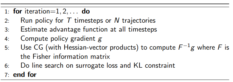
which has the following benefits and has been popular:

Policy gradient approach
Uses surrogate optimization function
Automatically constrains the weight update to a trusted region, to approximate where the first order approximation is valid
Empirically consistently does well

Monte Carlo Tree Search

Essentially it is Model-Based Reinforcement Learning, which aims to do:

given experience, learn the model (i.e. transition and/or reward function)
then use the model to plan and construct a value function or policy
- since now you have that simulator model, you can also do model-free RL at this step

(whereas all the previous sections were directly learning the value function or policy from experience, which Model-Free RL)

Graphically, model-based RL is trying to answer the following questions:

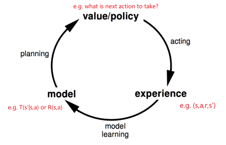
where the trick of this against the Model-Free approach is that, when finding the next action, we do not have to compute the full value function/policy (as in Model-Free approaches). We only need to find the next single action, which is exploited by the MCTS algorithm.

Advantages:

Can efficiently learn model by supervised learning methods
- e.g. for modeling transition function we need to spit out a distribution, and for reward, it is a regression problem.
Can reason about model uncertainty
- e.g.upper confidence bound methods for exploration/exploitation trade offs
can be good at transfer learning if only the reward function is changed.
- i.e. if you have the model learnt, then you can zero-shot transfer

Disadvantages:

First learn a model, then construct a value function. This means there are potentially two sources of approximation error
- e.g. like imitation learning, we could have compounding errors

Model Learning

Recall that a model is a representation of an MDP $(S,A,P,R)$, which can be parametrized by $\eta$:

\[M = (P_{\eta}, R_{\eta} ), \quad \begin{cases} s_{t+1}\sim P_\eta(S_{t+1}|S_t,A_t) \\ r_{t+1} = R_\eta(S_t,A_t) =R_\eta(R_{t+1}|S_t,A_t) \end{cases}\]

assuming that the state space and action space are already known. Typically we also assume that state transitions and rewards are independent:

\[\mathbb{P}(S_{t+1},R_{t+1}|S_t,A_t) = P_{\eta}(S_{t+1}|S_t,A_t)R_{\eta}(R_{t+1}|S_t,A_t)\]

Goal: estimate a model $M_\eta$ from experience ${ S_1,A_1,R_1, …,S_T }$. This becomes a supervised problem to consider input of: $$

\begin{align} S_1,A_1&\to R_1,S_2
S_2,A_2&\to R_2,S_3
&… \end{align}

$$ since there are two outputs, we can consider:

learning $s,a\to r$ being a regression problem (output a scalar)

learning $s,a\to s’$ being a density estimation problem (e.g. a vector of size $\left\vert S\right\vert$ with each slot being a probability)

then the loss functions could be mean-square error and KL divergence, and etc.

Example Models:

Table Lookup Model, e.g. if state and actions are discrete, we can just count them: $$

\hat{P}(s’	s,a) = \frac{1}{N(s,a)} \sum\limits_{t=1}^{T}\mathbb{1} {s’	S_t=s,A_t=a}\
\hat{R}(r	s,a) = \frac{1}{N(s,a)} \sum\limits_{t=1}^{T}R(S_t=s,A_t=a)

Linear Expectation Model
Linear Gaussian Model
Gaussian Process Model
Deep Belief Network Mode
Bayseian DNN
etc.

For instance, consider using a table lookup model shown above and we have the following data:

Data	Table Lookup Model

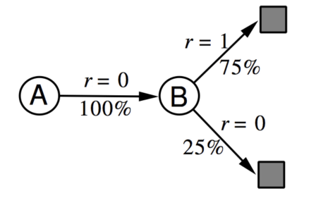where:

for simplicity we assume there is only one action
since we are storing averages and counts, essentially table look up decides:
- $R(S=a)=0$ since all the time the immediate reward is zero
- $R(S=b)=0.75$ on average

What would happen if we used a MC/TD estimate of the value $V(A),V(B)$?

MC estimate considers full track, but since the track with $A$ is still zero:
- $V(A)=0$
- $V(B)=0.75$
TD(0) estimate with infinite sampling propagates information by $V(A)=r+V(B)$ since $A\to B$ happens 100\%.
- $V(B)=0.75$ still the same
- $V(A)=0+0.75=0.75$ is different
essentially the difference arises because TD assumes/factors in the MDP process, whereas the MC method does not.

However, if we used our simulated model and sampled from it, you could see the following data

Data	Table Lookup Model	Sampled Data

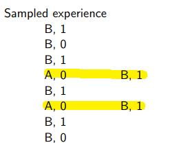where notice that in this case, if you were to estimate a value function using MC method (e.g. for planning), you will get:

$V(A)=1$ instead
$V(B)=0.75$ remains the same

notice that value functions now becomes closer to our TD estimates.

Planning with a Model

Once we have a learnt model, we can:

sample experience from model $(S,A,P_\eta,R_\eta)$
apply planning algorithms
- model-free RL to samples
  - e.g. MC control/policy iteration
  - e.g. SARSA, Q-Learning
- Tree search!

However, if the model $(S,A,P_\eta,R_\eta)$ is imperfect, then obviously the performance of your planning will be limited by your model.

in those cases it is important to know where it has gone wrong, e.g. by reasoning about its uncertainty (see previous section), before switching back to use model-free RL

But for here, we will focus on having a reasonbly good model, and how we can use tree search algorithms to compute the next step without explictly modelling the value functions.

Forward Search

The idea here is simple. Since we have a model that can spit out next state and rewards, we can build a tree by trying out different actions:

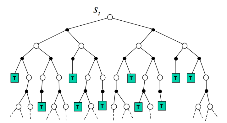
But then the question is, what is the next action to take if we are currently at $s_t$? For that we need to construct a value of the next actions, and one way is to consider:

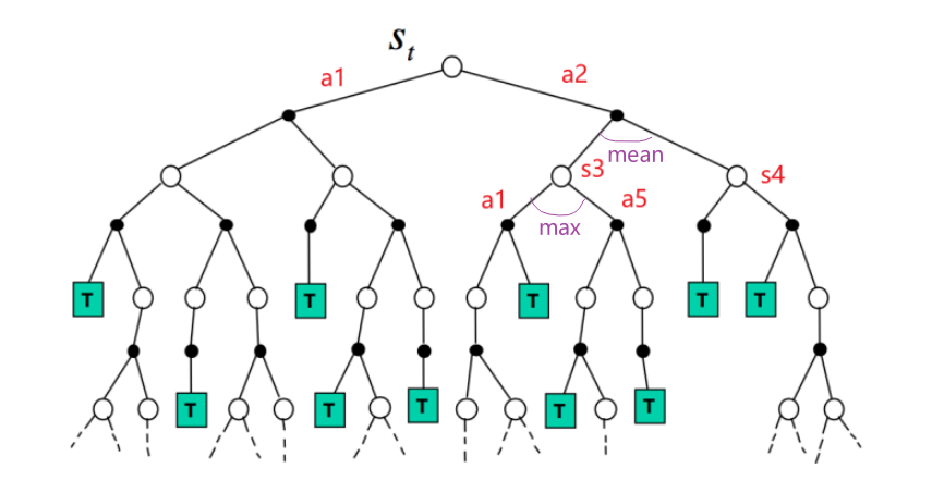
namely:

the value of the action is the mean of its future states
the value of a state is the max of its actions

Why might this be helpful? Notice that we don’t need to solve whole MDP, just sub-MDP starting from the current state!

However, to compute this at every step would be expensive. Do we have other approaches?

Simulation-Based Search

On the other hand, we can also utilize the model-free approaches, so that given a model $M=(S,A,P_\eta,R_\eta)$ we can:

given a policy $\pi$
sample experience ($K$ episodes) using the model: $$

{ S_t^{k},A_t^{k},R_{t}^{k}, …,S_T^{k} }{k=1}^{K}\sim M\eta

$$ do model-free control algorithsm treating those simulated experience to be real:
- Monte-Carlo Control (e.g. policy iteration) $\to$ Monte-Carlo Search
- SARSA $\to$ TD-Search

Simple Monte-Carlo Search

Since we are considering MC methods, then the idea is:

Given a model $M_\eta$ and a simulation policy $\pi$
for each action $a \in A$
1. simulate $K$ episodes from current state $s_t$ by considering all possible next actions, but then follows $\pi$: $$
  
  {s_t,a,R_{t+1}^{k},S^{k}{t+1},\pi(S^{k}{t+1}), …, S_T^{k}}{k=1}^{K}\sim M\eta,\pi
  
  $$
2. from this, we can compute the $Q^{\pi}$ function for each possible next action: $$
  
  Q^{\pi}(s_t,a) = \frac{1}{K} \sum\limits_{k=1}^{K} G_t^{k}(a)
  
  $$ for $G_t^{k}$ is the discounted reward of the $k$-th episode after following action $a$.
Then the current best action is: $$

a_{t} = \arg\max_{a} Q^{\pi}(s_t,a)

$$ which is like one-step of policy improvement

But can we do better by finding an optimal policy instead of only improving by one-step?

Monte-Carlo Tree Search

Recall that we can compute the optimal policy by considering the expectimax tree that we have shown before:

however, the size of this tree scales as $O((\vert S\vert \vert A\vert )^{H})$ for a height of $H$. Therefore, doing this at each step would be computationally intractable.

Instead, we consider a more computationally efficent way to approximate this full tree.

Heuristics: instead of simulting all possibilities, we can Iteratively construct and update tree by performing $K$ simulation episodes starting from the root state (i.e. $K$ rollout trajectories).

note that for this to work we need to have a “good” policy while generating those trajectories, which we shall discuss next

in fact, one key difference here against the Smple MC Search is that the policy generating each rollouts would be improving as well

Then, after the search is finished, simply consider: $$

a_t=\arg\max_a Q^\pi(s_t,a)

$$ note that as the policy $\pi$ genearing those trajectories improves, eventually this will converge to $\pi \to \pi^{}$ and $Q^{\pi} \to Q^{}$.

So we will consider two main changes as compared to the simple MC search:

rolling out $K$ trajecories will involve changing policies as well
To evaluate the value of a tree node $i$ at state action pair $(s, a)$, average over all rewards received (instead of max and average) from that node onwards across simulated episodes in which this tree node was reached

The key unasnwered question is: How to select what action to take during a simulated episode? Upper Confidence Tree Search!

UCT: borrow idea from bandit literature and treat each node where can select actions as a multi-armed bandit (MAB) problem

i.e. want to rollout more on actions that previously looked good, and spend less time on actions that previously looked bad

Therefore, we consider maintaining an upper confidence bound over reward of each arm $s,a$ of an episode $i$:

\[U(s,a,i) = \hat{Q}(s,a,i) + c\sqrt{\frac{\log(N(s))}{N(s,a)}}\]

for $\hat{Q}(s,a,i)$ is just an average reward by counting:

\[\hat{Q}(s,a,i)= \frac{1}{N(s,a,i)} \sum\limits_{k=1}^{K} \sum\limits_{u=t}^{T} \mathbb{1}(i\in \mathrm{episd.k})G_k(s,a,i)\]

so essentially we are treating each state node as a separate MAB. Then, using this, while simulating episode $k$ at node $i$, our “policy” is to select action/arm with highest upper bound to expand (or evaluate) in the tree:

\[a_{ik}=\arg\max U(s,a,i)\]

This implies that the policy used to simulate episodes with (and expand/update the tree) can change across each episode.

All in all, we will sample new episodes by:

Tree policy: pick actions for tree nodes to maximize $U(S, A)$, the upper confidence bound. e.g. use it until all next action has at least one sampled trajectory
Roll out policy: pick actions randomly, or another policy. This is used when we met a state with no data

For a more detailed example of this, see the next section.

Case Study: GO

Go is 2500 years old and is considered as the Hardest classic board game:

However, in this case:

instead of a need to model the game, since all the rules are known, we do not need $M_\eta$ in this case, but only do MCTS.
since it is a two-player game, we consider a minimax tree (min value for opponent wining) instead of a expectimax tree

For instance, we can consider a reward function of: $$

R_{T} = \begin{cases} 1, & \text{if black wins}
0, & \text{if white wins} \end{cases}

\[and our aim is to, say let black win. Then for $\pi=(\pi_B,\pi_W)$:\]

V_\pi(s)=\mathbb{E}\pi\left[R_T|S=s\right]=\mathbb{P}[\text{black wins}|S=s]
V^*(s)=\max{\pi_B}\min_{\pi_W}V_\pi(s)

\[is a minimax problem. Then, essentially we consider sampling: |$t=1$ | $t=2$ | $t=3$ | $t=4$ | $t=5$ | |:----:|:----:|:----:|:----:|:----:| |<img src='/lectures/images/2022-09-30-STFCS234_Reinforcement_Learning/image-20220608173657.png' style='zoom:50%;'/>|<img src='/lectures/images/2022-09-30-STFCS234_Reinforcement_Learning/image-20220608172736.png' style='zoom:50%;'/>|<img src='/lectures/images/2022-09-30-STFCS234_Reinforcement_Learning/image-20220608172750.png' style='zoom:50%;'/>|<img src='/lectures/images/2022-09-30-STFCS234_Reinforcement_Learning/image-20220608172808.png' style='zoom:50%;'/>|<img src='/lectures/images/2022-09-30-STFCS234_Reinforcement_Learning/image-20220608172827.png' style='zoom:50%;'/>| where essentially for the first 5 sampled episodes: - the choice of opponent $\pi_W$ could be the agent at previous iteration (i.e. doing self-play) - the default policy could just be a random policy - we are performing the **default/rollout policy** for states that we have not seen before - perform **tree policy** with picking the upper confidence bound for states when we have seen all actions. > **Importance of self-play**: essentially the idea is that in the beginning, both current agent and the opponent (e.g. previous checkpoint) would have a similar level. Then this makes the *reward signal being more dense* and the model learns faster. And finally, for minimax tree, it looks like: <img src='/lectures/images/2022-09-30-STFCS234_Reinforcement_Learning/image-20220608174045.png' style='zoom:60%;'/> where we are trying to minimize the probability of white winning and maximize the probability of black winning (as we are learning the policy for black). **Advantages for MC Tree Search**: - Highly **selective** best-first search - Evaluates states dynamically (unlike e.g. DP) - Uses **sampling** to break curse of dimensionality (model tree) - Works for “black-box” models (only requires samples) - Computationally efficient, anytime, parallelisable # Safe Offline Reinforcement Learning As we have known so far, RL algorithms updates/improves itself via interacting with the environment, which in some cases might not be feasible. (e.g. training conversation bot, but since its interaction is with people, it is often not possible). <img src='/lectures/images/2022-09-30-STFCS234_Reinforcement_Learning/image-20220821203131.png' style='zoom:50%;'/> > Therefore, the aim of offline RL is to reuse previously collected datasets (e.g. ImageNet) to create a data-driven RL framework. Recall that some techniques we covered so far: | Technique | Visual | Comments | | :--: | :--: | :--: | | on-policy RL|<img src='/lectures/images/2022-09-30-STFCS234_Reinforcement_Learning/image-20220821203859.png' style='zoom:50%;'/> | continuously collects new data from environment | on-policy RL|<img src='/lectures/images/2022-09-30-STFCS234_Reinforcement_Learning/image-20220821204030.png' style='zoom:50%;'/>| collects new data after each policy update | off-policy RL(sometimes called batch RL) | <img src='/lectures/images/2022-09-30-STFCS234_Reinforcement_Learning/image-20220821204141.png' style='zoom:100%;'/> | we only have a buffer, no environment to interact with Note that just as in off-policy RL, the policy we trained $\pi_\beta$ is different the policy that is used for data collection $\pi$. --- In particular, consider solving the following problem: <img src='/lectures/images/2022-09-30-STFCS234_Reinforcement_Learning/image-20220821205626.png' style='zoom:80%;'/> where essentially: - we cannot interact with the student/let them do more experiments - hence, we only have two sets of data, which you can think of as:\]

\begin{cases} (s_{1} =\text{A}, a_{1} = \text{add}, a_{2} = \text{multiply}, r=95)
(s_{1} =\text{B}, a_{1} = \text{multiply}, a_{2} = \text{add}, r=92) \end{cases}

\[- so the task is to learn a policy **only from a fixed set of data** but can **generalize**/reason about unseen cases In addition to produing a new policy: > Safe Offline/Batch RL considers the following guarantee. Given past experience from some current policy $\pi$, we want to produce a new policy $\pi_\beta$ that > - with the probability at least $1 - \delta$, will not be worse than $\pi_\beta$ > - guarantee should not contingent on tuning any hyperparamters > > In general, we will be thinking of the **confidence** ($1-\delta$) we have on our predicted expected outcome using our policy $\pi_\beta$. This is particularly useful in high stakes domain (e.g. medicine). Finally, just to make the task clear: > **Task**: given some dataset $D$, we want to learn the best possible policy $\pi_e$ from it. Notice that sometimes learning a very good policy might not even be possible if $D$ contains no good data (e.g. only visiting the first few rooms in Montezuma's Revenge). In general, it depends on the coverage and will be discussed in section [Importance Sampling for Policy Evaluation](#Importance Sampling for Policy Evaluation). ## Safe Offline RL Formulation We will consider the following notation for consistency: - Our Policy $\pi$: $\pi(a) = P(a_t = a\vert s_t=s)$ - Trajectory: $T=(s_{1}, a_{1}, r_{1}, s_{2}, a_{2}, r_{2}, ..., s_{L}, a_{L}, r_{L})$ - Historical/Training Data: $D= \{ T_1, T_2, ..., T_n \}$ - Behavioral policy used to generated the data $D$: $\pi_b$ - Objective:\]

V^{\pi} = \mathbb{E} \left[ \sum\limits_{t=1}^{L} \gamma^{t} R_{t}

\pi \right]

\[(note that in many cases we may not know what $\pi_b$ is, especially when it is generated by human. This will be discussed at the end of the section, **but for now we assume that it is known**.) Then our aim is to have an algorithm $A$ learn a policy $A(D) \to \pi$ such that:\]

P(V^{A(D)} \ge V^{\pi_{b}}) \ge 1 - \delta

\[where the value of the behavioral policy $V^{\pi_{b}}$ can be estimated by MC estimation from the historical data, that $V^{\pi_b} (s) = (1/n)\sum\limits_{i=1}^{n} G_i(s)$ for $G_i(s)$ is the discounted return starting from state $s$ and ending at the end of the trajectory (and there are $n$ trajectories). Or, more commonly, we could consider some external baselines $V_{\min}$ as well, that:\]

P(V^{A(D)} \ge V_{\min}) \ge 1 - \delta

Realize that to find out $V^{A(D)}$, we need to take our old data to compute how good our new policy is, which is intrinsically off-policy.

Off Policy Policy Evaluation

Off Policy Policy Evaluation (OPE)

for policy $\pi_e$ we want to evaluate (e.g. $A(D)\to \pi$), convert historical data $D$ into $n$ independent and unbiased estimates of $V^{\pi_e}$

Essentially:

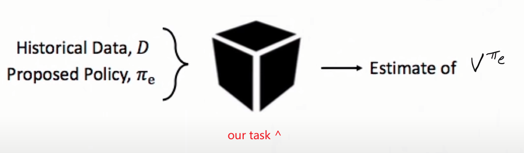
Therefore, our aim is:

Estimate value of policy $\pi_1$, $V^{\pi_1}(s)$, but given episodes $D= { T_1, T_2, …, T_n }$ generated under $\pi_2$

recall that $V^{pi}(s) = \mathbb{E}\pi [G{t} \vert s_t=s]$

we want to learn an unbiased estimate of $V^{\pi_1}(s)$

MC Off Policy Evaluation

Once mentioned unbiased, we should think of MC methods (as opposed to TD methods, which does sampling + bootstrapping). Additionally, this does not require the world to be Markov, which in realiy is often not the case!

First, we realize that because the policies are different $\pi_{1} \neq \pi_{2}$, we have two different distribution of states $\tau_{\pi_1}\neq \tau_{\pi_2}$ (otherwise the policies have the same value)

$\tau_{\pi_1}$	$\tau_{\pi_2}$

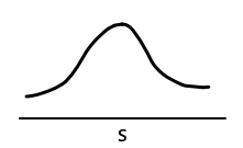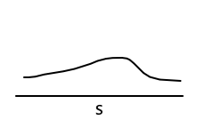Suppose that $\pi_{1}, \tau_{\pi_1}$ is known/collected. The idea is: how do we change the distribution to that they look alike? Importance Sampling!

essentially reweight the samples from $\tau_{\pi_2}$ so that samples from $\tau_{\pi_1}$

Importance Sampling for Policy Evaluation

Importance Sampling: goal is to estimate the expected value of a function $f(x)$ under some probability distribution $q(x)$, without knowing the distribution $q(x)$.

we want to know: $$

\mathbb{E}_{x \sim q}[f(x)]

$$

but we only have samples from $p(x)$, so that $x_1, x_2, …, x_n$ sampled form $p(x)$

(just swap $x \to s$, and $f(x)\to G_(s)$ you should see why this could be helpful)

Under few assumptions, we can use those samples to obtain an unbiased estimate of $\mathbb{E}_{x \sim q}[f(x)]$ $$

\begin{align} \mathbb{E}_{x\sim q}[f(x)] &= \int_{x} q(x)f(x)dx
&= \int_{x} \frac{p(x)}{p(x)}q(x) f(x) dx
&= \int_{x} p(x) \left[ \frac{q(x)}{p(x)} f(x)\right] dx
&\approx \frac{1}{n} \sum\limits_{i} \frac{q(x_i)}{p(x_i)}f(x_i),\quad x_i\sim p(x) \end{align}

\[so that essentially we sample data $x$ from $p(x)$, but reweigh the probability so that it looks the same as if the came from $x\sim q(x)$ Therefore, back in the case of RL, let $T_j$ be the episode $j$ of states actions and rewards (that are collected/sampled by $p(x)$):\]

T_{j} = (s_{j,1}, a_{j,1}, r_{j,1}, s_{j,2}, a_{j,2}, r_{j,2}, …, s_{j,L}, a_{j,L}, r_{j,L})

\[We need to first compute the ratio of $p(T_j\vert \pi_e)$ (the $q(x)$) over $p(T_j\vert \pi_b)$ (the $p(x)$):\]

p(T_j

\pi_e) =p(s_{j,1}) \prod_{i=1}^{L}\underbrace{p(a_{j,i}

s_{j,i})}{\mathrm{policy}} \underbrace{p(r{j,i}

s_{j,i},a_{j,i})}{\text{reward model}} \underbrace{p(s{j,i+1}

s_{j,i},a_{j,i})}_{\text{transition model}}

\[Then if we compute the ratio:\]

\begin{align} \frac{p(T_j|\pi_e)}{p(T_j|\pi_b)} &= \frac{p_{\pi_e}(s_{j,1})}{p_{\pi_b}(s_{j,1})} \prod_{i=1}^{L} \frac{p_{\pi_e}(a_{j,i}|s_{j,i})}{p_{\pi_b}(a_{j,i}|s_{j,i})}
&= \prod_{i=1}^{L} \frac{p_{\pi_e}(a_{j,i}|s_{j,i})}{p_{\pi_b}(a_{j,i}|s_{j,i})}
&= \prod_{i=1}^{L} \frac{\pi_e(a_{j,i}|s_{j,i})}{\pi_b(a_{j,i}|s_{j,i})} \end{align}

\[where - in the first equality, the over terms cancel since they do not depend on the policy chosen. - in the second equality, we are assuming the start state is the same for both policies Notice that the interpretation here is simple. Consider comparing the value of the policy using its start state, then: - we have a bunch of trajectories and computed expected rewards $(T_1,G_1),(T_2,G_2),...,(T_n,G_n)$ sampled from following $\pi_b$ - then the value of this policy $\pi_b$ can be estimated by $(1/n)\sum\limits G_i$ - but to estimate the value of $\pi_e$, we reweigh the probabilities by thinking how likely those trajectories are to be generated by $\pi_e$. So that if it is more likely, i.e. $p(T_j\vert \pi_e)>p(T_j\vert \pi_b)$, we will increase the weight using the above ratio. In general, $s_{j,1}$ can be any state as you can just rederive the above by considering $p(T_j\vert \pi_e,s=s_{j,1})$. Finally, this gives us the estimate:\]

\begin{align} V^{\pi_e}(s) &\approx \frac{1}{n} \sum\limits_{j=1}^{n} \frac{p(T_j|\pi_e,s)}{p(T_j|\pi_b,s)} G(T_j)
&= \frac{1}{n} \sum\limits_{j=1}^{n} \left(\prod_{i=1}^{L} \frac{\pi_e(a_{j,i}|s_{j,i})}{\pi_b(a_{j,i}|s_{j,i})} \right) G(T_j) \end{align}

\[Finally, since future cannot affect past rewards, we typically consider rewards only up to the timestep $t$ to reduce variance in our estimate:\]

\begin{align} V^{\pi_e}(s) &\approx \frac{1}{n} \sum\limits_{j=1}^{n} \left(\prod_{i=1}^{L} \frac{\pi_e(a_{j,i}|s_{j,i})}{\pi_b(a_{j,i}|s_{j,i})} \right) \left( \sum_{t=1}^L \gamma^T R_t^{i} \right) &\equiv \frac{1}{n} \sum\limits_{j=1}^{n} w_i \left( \sum_{t=1}^L \gamma^T R_t^{i} \right) \end{align}

\[note than since sometimes the importance weights $w_i$ can become very small, there is a Weighted Importance Sampling (WIS) algorithm to deal with this tha basically switch $1/n$ ratio to $1/\sum w_i$ (however, this increase bias while reduces variance) Now, what are the assumptions used to make IS work? You might notice the term $\frac{\pi_e(a_{j,i}\vert s_{j,i})}{\pi_b(a_{j,i}\vert s_{j,i})}$ could have gone badly, and it is extactly the case > **Importance Sampling Assumptions**: since we are reweighing samples from $\pi_b$, if we have distributions that are non-overlapping, then this will obviously not work. > - in particular, if we have any single case that $\pi_b(a\vert s)=0$ but $\pi_e(a\vert s)>0$, then this will not work. > - therefore, for this to work, we want to have a large coverage: so that for $\forall a,s$ such that $\pi_e(a\vert s)>0$, you want $\pi_b(a\vert s)>0$. Intuively, this means that if $\pi_e$ is not too far off from $\pi_b$, then the importance sampling would work reasonably. ### Adding Controlling Variates Given some random variable $X$, we want to estimate $\mu = \mathbb{E}[X]$. - we have our estimator being $\hat{\mu}=X$ - unbiased estimator: $\mathbb{E}\left[\hat{\mu}\right]=\mathbb{E}\left[X\right]=\mu$ - variance of this estimator: $\mathrm{Var}\left[\hat{\mu}\right]=\mathrm{Var}\left[X\right]$ Now, we want to show that in many cases we can use some tricks to reduce the variance while still having an unbiased estimator. Consider another random variable $Y$: - let our new estimator be $\hat{\mu}=X-Y+\mathbb{E}[Y]$ - it is still unbiased because:\]

\mathbb{E}[\hat{\mu}] = \mathbb{E}[X-Y + \mathbb{E}[Y]] = \mathbb{E}[X] - \mathbb{E}[Y] + \mathbb{E}[Y] = \mathbb{E}[X]

\[- it however can get a lower variance:\]

\mathrm{Var}[\hat{\mu}] = \mathrm{Var}[X-Y+\mathbb{E}[Y]]=\mathrm{Var}[X-Y] = \mathrm{Var}[X] + \mathrm{Var}[Y] - 2 \mathrm{Cov}(X,Y)

\[therefore, we just need $2\mathrm{Cov}(X,Y) > \mathrm{Var}[Y]$ to lower the variance in total while not introducing bias. Note that this might sound like some free lunch, but it is not because we are using $Y$ that has some information about $X$ since $2\mathrm{Cov}(X,Y) > \mathrm{Var}[Y]$. --- Therefore, we can use this fact and use $X$ being the **importance sapmling estimator**, and $Y$ being a **control variate** build from an approxiamte model of the MDP (e.g. a Q value estimate). This gives a Doubly Robust Estimator (Jiang and Li, 2015) > **Doubly Robust Estimator**: robust to (1) poor approximate model/control variate, and (2) error in estimates of $\pi_b$ (importnace sampling) because: > - if the model is poor, the estimates $V^{\pi_b}$ is still unbiased > - if importance sampling could not see some $\pi_b$ state/actions, but the model/contorl variate is good, then MSE will still be low. And just to briefly show the equation:\]

DR(\pi_{e}

D) = \frac{1}{n} \sum\limits_{i=1}^{n} \sum\limits_{t=0}^{L} \gamma^{t} \underbrace{w_i}{\text{IS weights}} (R_t^{i} - \underbrace{\hat{q}^{\pi_e}(S_t^{i},A_t^{i})}{\text{Y}})+\gamma^{t} \rho_{t-1}^{i}\underbrace{\hat{V}^{\pi_e}(S_t^{i})}_{\mathbb{E}[Y]}

Finally, we can show the properties of those different algorithms empically by simulating a small grid world (e.g. 4x4 world), providing the algorithm with some data collected under polict $\pi_b$ and ask it to evaluate the value of some new policy $\pi_e$:

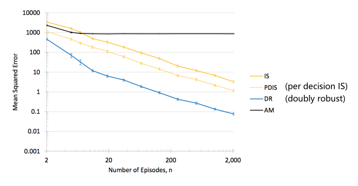
where:

the vertical axis is the MSE, which is $\hat{V}^{\pi_e}-V^{\pi_e}$ for $V^{\pi_e}$ is known beforehand since the world is simulated
so we want to get low MSE with small amount of data

High confidence Off-policy Policy Evaluation

Now, we have had some methods of how to obtain an OPE of $\pi_e$. The question is how confidence we are of our estimates?

High-confidence off-policy policy evaluation (HCOPE)

Use a concentration inequality to convert the $n$ independent and unbiased estimates of $V^{\pi_e}$ into a $1-\delta$ confidence lower bound on $V^{\pi_e}$

You can often think of such as confidence as the confidence used for RL exploration: how confident are we in terms of the new actions we are taking?

Essentially:

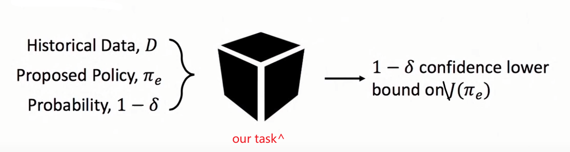
To be be able to know the confidence interval, we first need to revisit Hoeffding’s inequality:

Hoeffding’s Inequality: let $X_1, X_2, …, X_n$ be $n$ IID random variables such that $X_i\in[0.b]$. THen with the probability at least $1-\delta$: $$

\mathbb{E}[X_i]\ge \frac{1}{n} \sum\limits_{i=1}^{n} X_i - b \sqrt{\frac{\ln(1/\delta)}{2n}}

$$ where $X_i=\frac{1}{n}\sum\limits_{i=1}^{n} (w_{i} \sum\limits_{t=1}^{L} \gamma^{T} R_{t}^{i})$ in our case

However, the problem with applying this directly is that we can get very high $b$ since the weights $w_i$ might become big for rare but successful events.

for instance, if we you have 10,000 trajectories/samples, we could get a 95% confidence lower bound of the policy’s vlaue being $-5,8310,000$
whereas the true value would be $0.19$

Graphically:

IS weighted Return	Idea

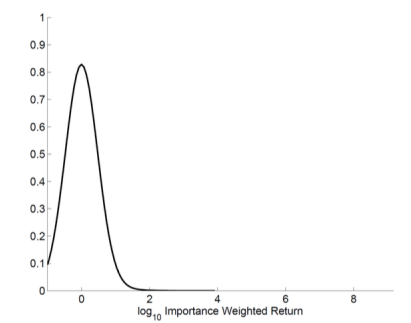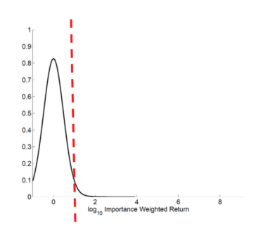where by cutting the large weights off, we will get a lower expected value but not have confidence interval exploding. Therefore, in practice, we can:

take 20% of the data to optimize the cutoff
use 80% of the data to compute lower bound

results for a certain policy on mountain climbing gives (true value $0.19$)

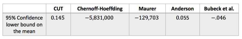
where the other columns are other concentration based methods.

Safe Policy Improvement

Safe policy improvement (SPI)

Use HCOPE method to create a safe batch reinforcement learning algorithm, by doing: $$

\pi = \arg\max_{\pi_e} V^{\pi_e}

$$ with some confidence intervals

Essentially:

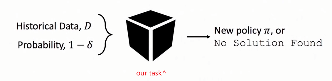
for instance, if there is too little data, we should be able to say no that we can have some new policy/improved policy is safe.

Practically, some current approach involve

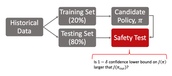
Note that this is a algorithm that only improves the policy for a single step. Other future areas/goals involve improving the policy over multiple steps.

General Offline RL Algorithms

A relevant content will be UCB CS285 on YouTube. link

Besides those safety constraints, there are also many other offline RL algorithms that are worth discussion. Before going to any details, we want to make certain high level ideas clear. Given this dataset $D$:

can offline RL perform better than the best behavior in $D$? Possibly yes, because of generalization: good behavior in one place may sufggst good behavior in another place
can offline RL learn the best policy just from $D$? Often no, because we might have very few or no samples in $D$ where we see traces of the best policy, hence it is not even possible.

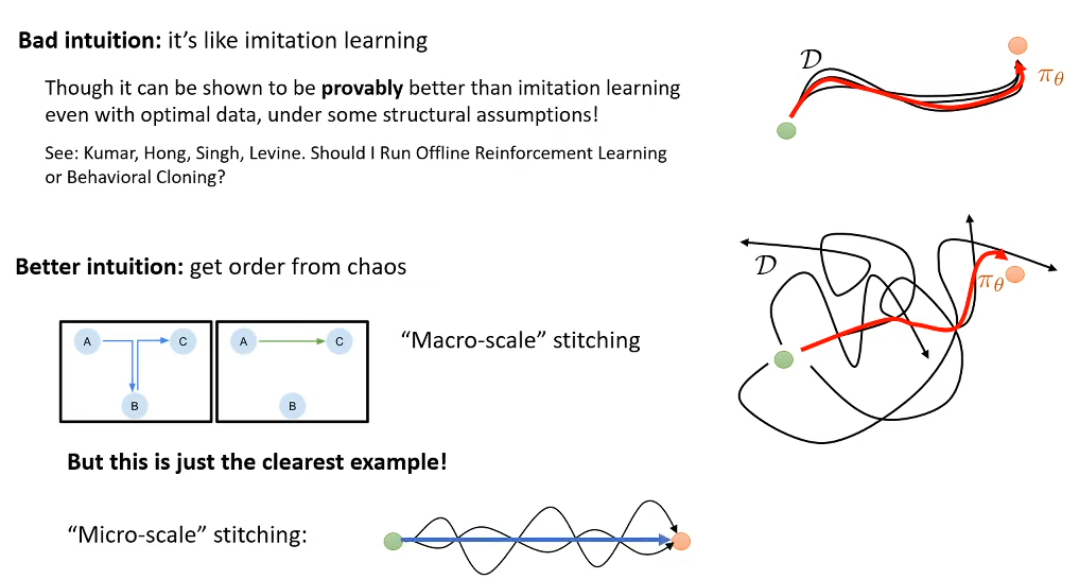
But more generally, we consider:

$D = {(s_i, a_i, s_i^{\prime}, r_i}$ the same as before
$\pi_b$ is the behavior policy creating the data $D$, so that $s \sim \mu_{\pi_b}(s)$ and $a \sim \pi_b(a\vert s)$
however, now we generally assume that $\pi_b$ is NOT known
we want to find a new policy $\pi_{\mathrm{new}}$ that can combine good decisions

And, as mentioned before, since $\pi_b \neq \pi_\mathrm{new}$ for $\pi_\mathrm{new}$ we want to learn, there is a problem of distribution shift

Distribution Shift for learning Value Functions in Offline RL: consider we are learning a value function $Q$. Idealy, if we want to learn $Q^{\pi_{b}}$, we consider the objective: $$

\min_Q \mathbb{E}{(s,a,s’)\sim D} \left[ \left(\underbrace{r(s,a) + \mathbb{E}{a’\sim \pi_b}[ Q(s’,a’)]}_{\mathrm{target}} - Q(s,a)\right)^2 \right]
\[in practice, we can only do: - using sample mean instead of expcted value (as usual) - can only sample $a' \sim \pi_{e}$ since we do not have the behavioral policy, hence we are doing:\]
\min_Q \mathbb{E}{(s,a,s’)\sim D} \left[ \left(\underbrace{r(s,a) + \mathbb{E}{a’\sim \pi_\mathrm{new}}[ Q(s’,a’)]}_{\mathrm{target}} - Q(s,a)\right)^2 \right]

$$ which we only expect to work if $\pi_\mathrm{new}(a\vert s) \approx \pi_b(a\vert s)$.

However, in reality we usually consider having: $$

\pi_{\mathrm{new}} = \arg \max_{\pi} \mathbb{E}_{a \sim \pi(a

s)} [Q(s,a)]

\[so that the $\pi_\mathrm{new}$ learnt usually ends up fooling us by adverserially picking large values in the (inaccurate) Q function estiamte. Graphically: | $\hat{Q}$ estimate of $\pi_\mathrm{new}$ | Actual Return of $\pi_\mathrm{new}$ | | :--: | :--: | | <img src='/lectures/images/2022-09-30-STFCS234_Reinforcement_Learning/image-20220826192651.png' style='zoom:60%;'/> |<img src='/lectures/images/2022-09-30-STFCS234_Reinforcement_Learning/image-20220826192630.png' style='zoom:60%;'/> | Therefore, what can we do this such a problem? ## Policy Constraint Methods A simple and a bit naive way is to consider a policy $\pi_\mathrm{new}$ such that:\]

\pi_\mathrm{new}(a

s) = \arg\max_\pi \mathbb{E}_{a \sim \pi(a

s)} [Q(s,a)],\quad \mathrm{s.t.} D_{KL}(\pi

\pi_b) \le \epsilon

\[and then continue with the Bellman update:\]

Q(s,a) \gets r(s,a) + \mathbb{E}{a’ \sim \pi\mathrm{new}} [Q(s’,a’)]

\[while this seems to solve distribution shift, there are several issues: 1. usually we don't know what $\pi_b$ is (e.g. human collected data) 2. if you are too close to $\pi_b$, then you cannot improve your policy, even if your data $D$ already has a large support/coverage (e.g. $\pi_b$ is uniformly random) But before we consider other methods, let us dive into more details about how/when this idea could work. Consider the case that you are at some state $s$ and given some rewards for some actions in your $D$: | Data | Fitted Q Function | Constrained New Policy $\pi$ | | :--: | :--: | :--:| |<img src='/lectures/images/2022-09-30-STFCS234_Reinforcement_Learning/image-20220826211857.png' style='zoom:100%;'/>|<img src='/lectures/images/2022-09-30-STFCS234_Reinforcement_Learning/image-20220826211906.png' style='zoom:80%;'/>|<img src='/lectures/images/2022-09-30-STFCS234_Reinforcement_Learning/image-20220826212034.png' style='zoom:80%;'/>| where: - the orange dots are the given $Q$ values - the middle fitted $Q$ function would give bad policy exploiting the tails - the last one seems better, but it is still giving a bit too high Q values to non-optimal actions Therefore, given this intution, we would prefer to have a support policy (instead of $\pi_b$) to look like: <img src='/lectures/images/2022-09-30-STFCS234_Reinforcement_Learning/image-20220826212548.png' style='zoom:50%;'/> so that KL-divergence would work the best. This means we consider the support constraint:\]

\pi(a

s) \ge 0 \text{ only if } \pi_b(a

s) \ge \epsilon

\[which we can approximate using methods such as MMD as we don't have $\pi_b$ directly, but in practice they are very difficult to implement. --- Finally, here we show some examples of how to explicitly include policy constraints in practice: 1. consider the case of using Actor Critic methods, where the actor $\pi_\theta(a\vert s)$ has the objective:\]

\theta \gets \arg\max_\theta \mathbb{E}{s \sim D} \left[ \mathbb{E}{a\sim \pi_\theta(a

s)} [Q(s,a)] \right]

\[but for KL divergence constraint, we want:\]

D_{KL}(\pi_\theta

\pi_b) = \mathbb{E}{\pi\theta}[\log \pi_\theta(a

s) - \log \pi_b(a

s)] = \mathbb{E}{\pi\theta}[\log \pi_b(a

s)] - \mathcal{H}(\pi_\theta)

\[for $\mathcal{H}(\pi_\theta)$ is the entropy. We can then easily convert constrained problems into unconstrained optimization using Legrange's Methods:\]

\theta \gets \arg\max_\theta \mathbb{E}{s \sim D} \left[ \mathbb{E}{a\sim \pi_\theta(a

s)} [Q(s,a)+ \lambda\log \pi_b(a

s)] + \lambda \mathcal{H}(\pi_\theta(a

s)\right]

\[for $\lambda > 0$ is the Legrange Multiplier. But again, this means you need to know $\pi_b$, which unfortunatly you cannot avoid and commonly is done by doing behavioral cloning on the dataset $D$. 2. Another simple way is to change the reward function:\]

\bar{r}(s,a) = r(s,a) - D_{KL}(\pi

\pi_b)

\[which can not only makes current behavior more consistent, but also accounts for future behavior/divergence. This form of approach is called Behavior Regularized Offline RL But again, generally best offline RL algorithms today do not use these methods. ## Implicit Policy Constraint Methods Recall the for policy constraint, we are considering the problem:\]

\pi_\mathrm{new}(a

s) = \arg\max_\pi \mathbb{E}_{a \sim \pi(a

s)} [Q(s,a)],\quad \mathrm{s.t.} D_{KL}(\pi

\pi_b) \le \epsilon

\[and by using Legrange Duality and solving for the optimal policy we get:\]

\pi^{\star}(a

s) = \frac{1}{Z(s)} \pi_b(a

s) \exp\left( \frac{1}{\lambda}A^{\pi}(a

s) \right)

\[which intuitively means that: - suboptimal actions are exponentially less likely - even for very high advantage $A$, if the action is rare in behavior policy $\pi_b$ then this is bad - $\lambda$ can be often treated as a hyperparameter or tuned Since this is the best policy, then it means we can approximate using weighted maximum likelihood:\]

\pi_\mathrm{new}(a

s) = \arg\max_\pi \mathbb{E}_{(s,a)\sim \pi_b(a

s)} \left[ \log\pi(a

s) \underbrace{\frac{1}{Z(s)}\exp\left(\frac{1}{\lambda}A^{\pi_{\mathrm{old} (s,a)}}\right)}_{\text{weights }w(s,a) } \right]

\[where the advantage function is just given by critic. In a sense this is a **weighted behavior cloning**, so that it is imitating the good actions more than the bad actions. To implement this, all you need to do is to change slightly the actor-critic training: 1. train critic as usual with the loss:\]

L_C(\phi) = \mathbb{E}{(s,a,s’)\sim D} \left[ (Q\phi(s,a) - ( r(s,a)+\gamma \mathbb{E}{a’\sim \pi\theta(a’

s’)}[Q_\phi(s’,a’)] ))^{2} \right]

\[2. train actor with our constrained loss:\]

L_A(\theta) = - \mathbb{E}_{(s,a)\sim \pi_b(a

s)} \left[ \log\pi_\theta(a

s) \frac{1}{Z(s)}\exp\left(\frac{1}{\lambda}A^{\pi_{\mathrm{old} (s,a)}}\right) \right]

\[3. update the actor and critic loss via gradient descent alternatingly More details see this paper [Nair, Dalal, Gupta, Levine. 2020](https://arxiv.org/pdf/2006.09359.pdf). Some more caustions of this method include the fact that you could still query OOD actions **during** training (constraints respected only at expectation), which could happen when computing the target value for updating critic or when estimating the advantage function. ### Implicit Q-Learning Is there a way to avoid OOD actions while learning the Q function? This serves for the motivation of the work [Kostrikov, Nair, Levine. 2021](https://arxiv.org/pdf/2110.06169.pdf), with the idea being formulated as follows. 1. we consider instead of the following update rule\]

Q(s,a) \gets r(s,a) + \mathbb{E}{a’ \sim \pi{\mathrm{new}}}[Q(s’,a’)]

\[we view it as\]

Q(s,a) \gets r(s,a) + \underbrace{V(s’)}_{\text{just another neural network}}

\[2. next, we recall that a batch constrained TD updates considers:\]

L(\theta) = \mathbb{E}{(s,a,s’)\sim D} \left[ ( r(s,a) +\gamma \max{\pi_b(a’

s’)>0}Q_{\hat{\theta}} - Q_\theta(s,a))^2 \right]

\[thefore, to mimic this behavior, we have two choices: - using expectile loss $L_2^{\tau}$ directly on $Q$, so that we have:\]

  L(\theta) =  \mathbb{E}_{(s,a,s')\sim D} \left[ L_2^\tau( r(s,a) +\gamma \max_{\pi_b(a'|s')>0}Q_{\hat{\theta}} - Q_\theta(s,a)) \right]
  
  $$
  (explaination of expectile loss seen in the next paragraph) but this have a drawback, and that is since each update sample contains $(s,a,s')$, it includes the stochasticity of a sample getting high reward because of *lucky* transition to $s'$ instead of doing the correct action $a$. This we do not want to have in our learned critic/policy.
- using expectile loss to first fit a value function $V$:
  $$
  
  L_V(\psi) = \mathbb{E}_{(s,a) \sim D} \left[ L_2^{\tau}(Q_{\hat{\theta}}(s,a) - V_\psi(s)) \right]
  
  $$
  which uses expectile because we want $V_\psi$ to learn the upper end in the distribution to approximate $\max Q_{\hat{\theta}}$, and then we simply use that and do:
  $$
  
  L_Q(\theta) = \mathbb{E}_{(s,a,s')\sim D} \left[ ( r(s,a) +\gamma V_\psi(s')- Q_\theta(s,a))^{2} \right]
  
  $$
  which notice that we do avoided the case of lucky transition while we are training the $V_\psi$ approximation function.

note that one concern could be: “before we were worried about $Q(s,a)$ giving unlikely large values, but now we are fitting $V$ to get large values?” The answer is no, because the previous problem is due to the fact that it comes from OOD actions, but here $V$ is trained only in data and hence have no overestimation problem.

Finally, we graphically provide interpretation of why this expectile and the $V_\psi$ function would work. Consider the case that you have multiple trajectories, and for a continous/large action space, you might see:

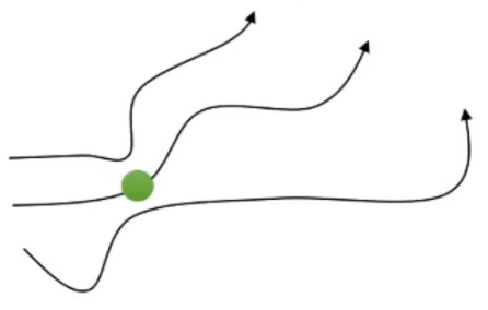
Suppose you are on the green circle state. Even though there is only one action, you can still consider the value of this state being a distribution because its neighbor states/trajectories has a different action. Therefore, this leads up to the following value function distribution from your data:

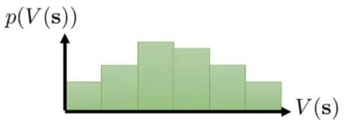
where the probability of each value is induced by actions (e.g. neighbor/similar states) only. Then, if we go back to the objective of fitting a value function:

\[V = \arg\min_{V} \frac{1}{N} \sum\limits_{i=1}^{N} L(V(s_i), Q(s_i,a_i))\]

taking:

MSE Loss	Expectile Loss, $x=V_\psi(s)-Q_{\hat{\theta}}(s,a)$
$(Q_{\hat{\theta}}(s,a) - V_\psi(s))^{2}$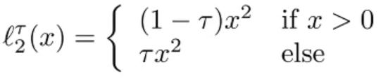

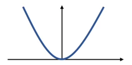This means that when fitting the $V$:

MSE Loss	Expectile Loss

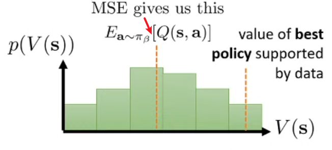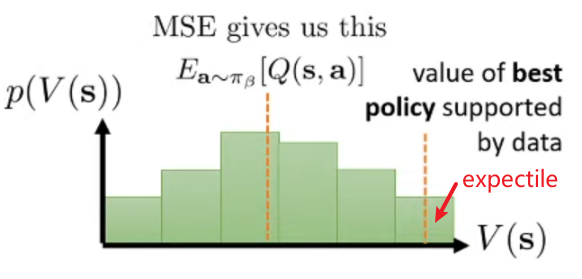Finally, when this $V$ learns from the good actions at each state, it can be effectively combined to our $Q$ network from which we can extract the policy, as indicated in the paper/algorithm overview above.

Conservative Q-Learning Methods

Instead of trying to fix actors by asking them not to sample OOD actions, CQL methods try to repair critic directly. Specically, recall that our previous problem is:

$\hat{Q}$ estimate of $\pi_\mathrm{new}$	Actual Return of $\pi_\mathrm{new}$

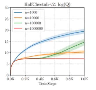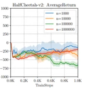SO essentially, if the idea is to push down large Q values in general (as they are likely to be wrong), being rather pessimistic:

Fitted Q vs Real Q	Conservative Q-Learning

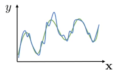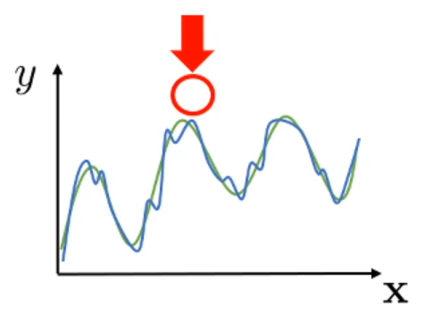a simple idea to achieve this is to consider the Q value objective:

\[\hat{Q}^{\pi} = \arg\min_{Q} \,\,\max_\mu \underbrace{\alpha \mathbb{E}_{s\sim D, a \sim \mu(a|s)}[Q(s,a)]}_{\text{push down big Q-values}} + \underbrace{\mathbb{E}_{(s,a,s')\sim D} \left[ (Q(s,a) - (r(s,a)+ \mathbb{E}_\pi[Q(s',a')]))^{2} \right]}_{\text{regular objective}}\]

where notice that $\mu$ is picked so that $Q$ looks large, and then the final $Q$ is picked to minimize those. Hence in theory, it can be shown that if you pick a large enough $\alpha$, you can show that $\hat{Q}^\pi \le Q^{\pi}$ for the true $Q^\pi$.

But in reality, this generally pushes down all the Q values, which could be a little too pessimistic. Therefore, we could maybe do better by considering:

\[\hat{Q}^{\pi} = \arg\min_{Q} \,\,\max_\mu \underbrace{\alpha \mathbb{E}_{s\sim D, a \sim \mu(a|s)}[Q(s,a)]}_{\text{always pushes down Q}} - \underbrace{\alpha \mathbb{E}_{(s,a)\sim D}[Q(s,a)]}_{\text{push up (s,a) in data}} + \underbrace{\mathbb{E}_{(s,a,s')\sim D} \left[ (Q(s,a) - (r(s,a)+ \mathbb{E}_\pi[Q(s',a')]))^{2} \right]}_{\text{regular objective}}\]

where this is the CQL objective $L_{\mathrm{CQL}}$, such that:

for $(s,a)$ samples in the dataset, the push up and down term will cancel the effect out and have little net effect
for $(s,a)$ samples not in the dataset, the first term will push them down but the second will push up actions in dataset. This means that for the next time, $\mu$ would tend to select actions similar to the dataset since they have large values.

Therefore, the intuition is that :

if you meet OOD actions, the two terms will act to push them back to in-distribution actions.
once they are in-distribution, the two terms more or less cancel out.

As a result:

we no longer directly guarantee that $\hat{Q}^{\pi}(s,a) \le Q^\pi(s,a),\forall (s,a)$
but we do guarantee that their expected value (i.e. value function) is bounded $\mathbb{E}{\pi(a\vert s)}[\hat{Q}^{\pi}(s,a)] \le \mathbb{E}{\pi(a\vert s)}[Q^{\pi}(s,a)], \forall s \in D$

Then, as shown in the paper Kumar, Zhou, Tucker, Levine. 2020, implement RL algorithm with CQL:

update $\hat{Q}^{\pi}$ w.r.t $L_{\mathrm{CQL}}$ using the dataset
update your policy $\pi$:
- if actions are discrete then simply: $$
  
  \pi(a|s) = \begin{cases} 1, \text{if } a=\arg\max_a \hat{Q}(s,a)
  0 , \text{otherwise} \end{cases}
  
  $$
- if actions are continous, then you usually have to fit another policy network $\theta$: $$
  
  \theta \gets \theta + \alpha \nabla_\theta \sum_i \mathbb{E}{a \sim \pi\theta(a s)}[\hat{Q}(s_i,a)]
  
  $$ which is basically like an actor-critic method.

Finally, to pick a $\mu$, we can first consider adding a max-entropy regularization term in our objective:

\[\begin{align*} \hat{Q}^{\pi} &= \arg\min_{Q} \,\,\max_\mu \alpha \mathbb{E}_{s\sim D, a \sim \mu(a|s)}[Q(s,a)] - \alpha \mathbb{E}_{(s,a)\sim D}[Q(s,a)] - \overbrace{\mathcal{R}(\mu)}^{\text{regularizer}} \\ &\quad + \mathbb{E}_{(s,a,s')\sim D} \left[ (Q(s,a) - (r(s,a)+ \mathbb{E}_\pi[Q(s',a')]))^{2} \right] \end{align*}\]

then with the choice of taking $\mathcal{R}=\mathbb{E}_{s\sim D}[H(\mu(\cdot \vert s))]$, we will have an optimal choce with $\mu(a\vert s) \propto \exp(Q(s,a))$ and hence: $$

\mathbb{E}_{a \sim \mu(a

s)} [Q(s,a)] = \log \sum\limits_{a} \exp(Q(s,a))

$$ so that:

for discrete actions, we can just caulcate directly $\log \sum\limits_{a} \exp(Q(s,a))$
for contionus actions, we can estimate $\mathbb{E}_{a \sim \mu(a\vert s)} [Q(s,a)]$ by using importance sampling

Model-Based Offline RL

All the previous mentioned methods are model-free, i.e. we do not have a world model getting us the transitions/rewards. In the context of offline RL, model-based methods can be pretty useful as you can:

train a wolrd model using your data $D$
use that model to do planning directly or learn a policy from it

Usually, model-based RL methods work as follows:

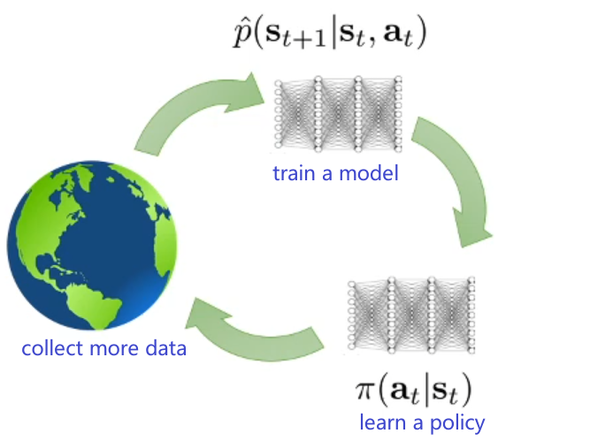
But since we cannot collect more data in offline RL, it means that:

| | | | :—: | :—: |

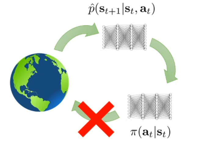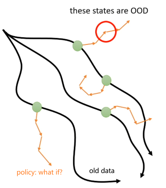so that essentially we are facing the same problem as those OOD actions in Q value estimates: now we are facing the threat that our policy could adversarially pick actions and transit to OOD states which the model could have some erroneously high values.

Therefore, the general intuition for this is to apply some kind of penalty for policys that exploit too many OOD states/actions.

Model-based Offline Policy Optimization

There are two papers on this topic of thought, which is:

MOPO: Model-based Offline Policy Optimization (2020)
MOReL: Model-based Offline Reinforcement Learning (2020)

where both of which modifies the reward function to trick the policy to stick more of less to data we have.

Uncertainty Penalty: we would like to modify the reward function to penalize the policy for going into states that might be incorrect (due to inaccuracies in the learned model). Therefore, we in general consider: $$

\tilde{r}(s,a) = r(s,a) + \lambda u(s,a)

$$ for $u$ is an uncertain penalty term.

While this sounds easy, it is usually hard to adjust the penalty term to make it work. Intuitvely, we would want:

Before Penalty	After Penalty

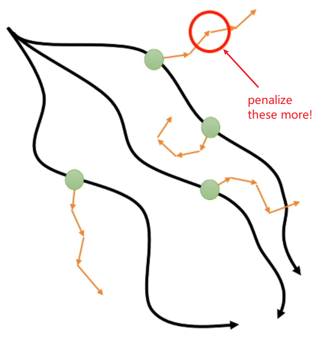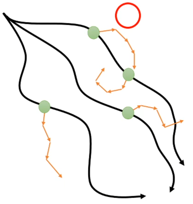This means that this penalty term needs to be at least as large as the error the model makes at those erroneous states (hence to provide incentive for the policy to not exploit them). So how do we quantify this?

one simple idea is to use ensemble disagreement: we train an ensemble of world models, and quantify the error by looking at the disagreement between the models.
but of course there are other ways as well

Consider we are learning a policy $\hat{\pi}$, then in the MOPO paper it is proven that:

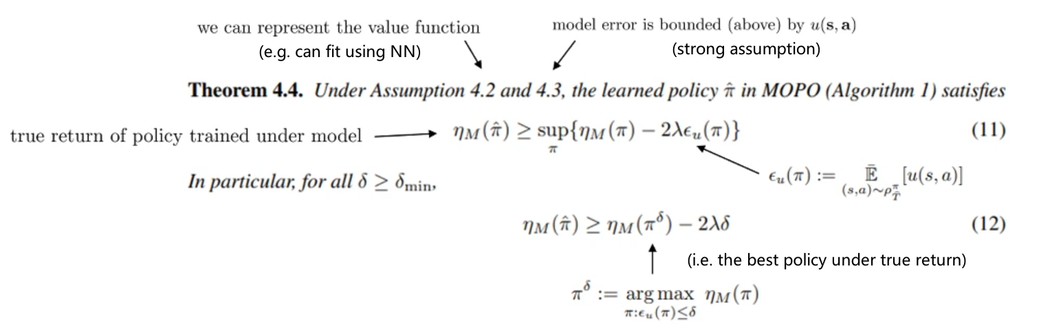
where $M$ is the world model we trained, and $\nu$ measures the true return. This basically gave two important implications. As we can substitute the policy $\pi$ term:

Our learned policy can improve upon the behaviorial policy (in terms of the true return): $$

\nu_M(\hat{\pi}) \ge \nu_M(\pi_b) - 2 \lambda \epsilon_u(\pi_b)

$$
We can also quantify the gap between the learned policy and the true optimal policy in terms of model error: $$

\nu_M(\hat{\pi}) \ge \nu_M(\pi^{\star}) - 2 \lambda \epsilon_u(\pi^{\star})

$$ and notice that if our model $M$ is very accurate, then $\epsilon_u$ is small and we are close to the optimal policy.

Conservative Model-Based RL

see the COMBO paper for more details

Intuition: just like with CQL we can minimize the Q-value of OOD policy actions, we can minimize the Q-value of model for OOD state-action tuples.

\[\begin{align*} \hat{Q}^{k+1} &\gets \arg\min_{Q} \beta ( \overbrace{\mathbb{E}_{(s,a) \sim \rho(s,a)}[Q(s,a)]}^{\text{push down}} - \overbrace{\mathbb{E}_{(s,a) \sim D}[Q(s,a)]}^{\text{push up}} )\\ &+ \frac{1}{2} \mathbb{E}_{(s,a,s') \sim d_f}[ (Q(s,a) - \mathcal{B}^\pi \hat{Q}^{k}(s,a))^{2} ] \end{align*}\]

where $\rho(s,a)$ is from our model $M$, and $\mathcal{B}^\pi$ is a Bellman operator. This tries to make the Q-values from the models be worse, but Q-values from the dataset be better. Therefore,

if the model produces something that looks different from the dataset, then this objective can have $Q$ makes it look bad
if the model produces something that is very close/indistinguishable from the dataset, then the first two terms cancel out

Trajectory Transformer

See Offline Reinforcement Learning as One Big Sequence Modeling Problem

The basic idea is:

consider trajectory as a whole, so we have a joint state-action model: $$

p_b(\tau) = p_b(s_1, a_1, …, s_{T}, a_T)

$$ which is the probabiliy under the behavioral policy.
then, we can use a transformer to model such a probability distribution.

Specifically, to deal with continuous states and actions, we discretize each dimension independently. Assuming N-dimensional states and M-dimensional actions, this turns $\tau$ into sequence of length $T(N +M +1)$:

\[\tau = ( ... , s_t^1, s_t^{2}, ..., s_t^{N},a_t^{1},a_t^{2},...,a_t^{M},r_t, ...), \quad t=1,...,T\]

so that subscripts on all tokens denote timestep and superscripts on states and actions denote dimension (i.e. $s_t^{i}$ is the $i$th dimension of the state at time $t$). While this choice may seem inefficient, it allows us to model the distribution over trajectories with more expressivity without simplifying assumptions such as Gaussian transition.

Then, we can model this as:

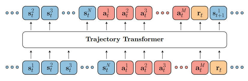
where we can then decode next state/actions given previous ones, and note that both the model and search strategy are nearly identical to those common in natural language processing.

Finally, to do planning, you need to keep in mind to take the action probabilities into account, so that you avoid OOD actions. But otherwise, you can:

just use Beam search, but to promote non-myoptic chioces:
1. given the current sequence (e.g. upto time stamp 3), sample the next $K$ tokens from the model (which means they are sampled from $p_b$)
2. store the top $K$ tokens with highest cumulative reward $\sum_{t} r(s_t,a_t)$ instead of probability
3. continue
or you could even use MCTS

Why does/should this work?

generating high-probability trajectories avoids OOD states and actions already, since we are sampling from $p_b$ when decoding.
using a big model (e.g. transformers) tend to work well in offline mode

Summaries and Directions on Offline RL

If you want to to only train offline:

CQL: just one hyperparmeter and is well understood and widely tested
Implicit Q-Learning: more flexible (offline+online), but has more hyperparameters

If you want to train offline and finetune online:

not CQL because it tends to be too conservative
Adavantage-weighted Actor-Critic (AWAC) is widely used and well tested
Implicit Q-learning works well

If you are confident that you can train a good world model:

COMBO: similar properties from CQL but also benefits from being model-based
Trajectory Transformer: very powerful, but is extremly computationally expensive to train and evaluate

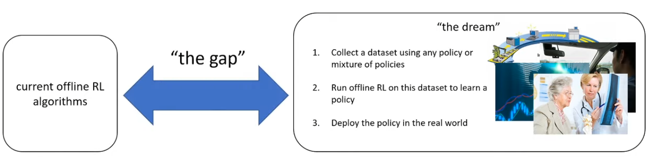
Finally, worthy mentions and challenages include that:

as compared to supervised training where you can train/test offline, offline RL upto today still have to test online (costly and maybe even dangerous)
statistically guarantees to help quantify distributional shift (currently pretty loose and incomplete)