Introduction and Logistics

Lecturer: Emily Tiberi ect2158@columbia.edu. Office hours: TBA or by appointment
Expectations
- your data analysis should be on Python or Mathematica, but not Excel
- Background physics: have taken any physics class at college level
- Time commitment: expected to spend on average less than 10 hours on your lab report each week
Absence Policy
- Attendance includes lab participation and lab report submission
- You are allowed two excused absences and one unexcused absence
Lab sessions:
- Each lab session will begin with a brief recap with the TA.
- Your lab group will collect raw data
- There will be in-lab discussions. Work in groups, analyze data and answer the discussion questions.
- You will have a week to finish the lab report
- bring your laptop, recommend recording raw data using excel and export
Lab report: your lab report should be your own, but all the others will be/can be collaborative
- your first week lab report will only be personal feedback, no grade
- there will be a rubric for lab reports
Grading: no quizzes, 90% lab report, and 10% in-lab discussion and participation (discussion with the TA)

Scientific Writing

Readers interpret prose more easily when it flows smoothly… From background rationale conclusion

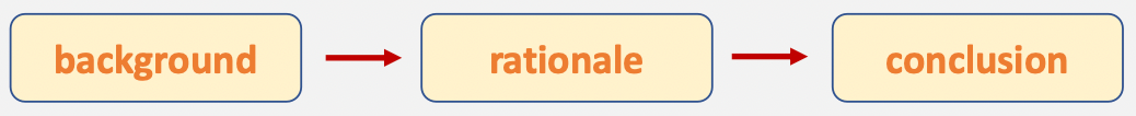
Don’t force the reader to figure out your logic – clearly state the rationale.
Clear writing is also concise writing. The report should be fairly brief (up to 4 pages).

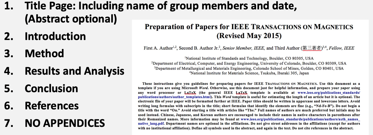
Your report should look like:

where

“References” most of the time empty
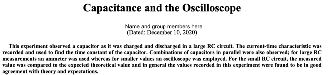
Abstract can be there, but is optional. For example
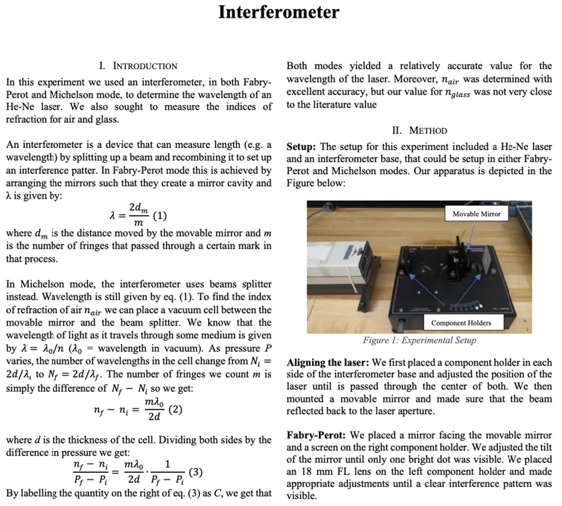
the introduction should usually be no more than half a page in single column
- describe the research question, why it is important, and what approaches (briefly) you used (optional: briefly mention the results if you want)
method: you really want to talk about your setup, including your apparatus and instruments used, any techniques, etc.
- this should be brief in general
results and analysis: the most important section in your report. You should succinctly give
- data obtained, graphs and tables
- how you calculated those quantities (if not obvious)
- comments on uncertainties. Why are certain error bars so big?
- is your result good?
conclusions: should be short. Contain your interpretation of the result, what you expected

Other notes for writing these reports

example, annotated lab reports are also provided in Courseworks

Error Analysis

When we measure any quantity, we cannot expect to measure it exactly = we will have errors/uncertainties in our experiment!

Therefore, instead of giving each of your friend $2.3684$ slices of pizza, you might say:

\[2.37 \pm 0.01 \quad \mathrm{slices}\]

note that

you may want to match the number of significant figures in your number and your uncertainty
usually keep up to 2 sig. figs.

Type of Errors

There are mainly two types of errors you get in your experiment

Statistical/Random Errors = no going around this, but are quantifiable

Due to random fluctuations from measurement to measurement

Can be reduced by taking more measurements, computing their mean and std

Systematic Errors = e.g. how you are measuring

Always bias the data in one direction

“do you best” to identify and correct it

Hard to quantify

How do we quantify statistical/random errors?

calculate mean $\bar{x}$, std $\sigma$
but also Standard Error of the Mean $\sigma_\bar{x}$ = uncertainty we have on our measured average = uncertainty in your lab report
\[\sigma_\bar{x} = \frac{s}{\sqrt{N}}\]
because each time one more measurement is taken, your mean will change. So here is that measure of “precision in our measurement of the mean”

What happens when you have different measurements all with different precisions and you want to combine them into a unique result?

For example, consider you are measuring a length with:

4 different rulers, each time measure once = $x_1\pm \sigma_1, x_2\pm \sigma_2,x_3 \pm \sigma_3,x_4 \pm \sigma_4$
4 different rulers, with each ruler you measured a lot of times, hence four averages $\bar{x}1 \pm \sigma{1}, \bar{x}2 \pm \sigma{2}, \bar{x}3 \pm \sigma{3}, \bar{x}4 \pm \sigma{4}$

And you want to report a single length measurement by a weigthed average of them. Then you can do this:

\[\bar{x} = \frac{\sum_i w_i x_i}{\sum_i w_i}, \quad w_i = \frac{1}{\sigma_i^2}\]

and then your error for this weighted mean is:

\[\frac{1}{\sigma^2} = \sum_{i=1}^N \frac{1}{\sigma_i^2}\]

(the more general way to derive those uncertainty is in the section: Error Propagation)

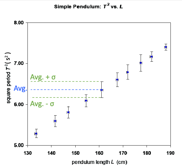
Confidence Intervals

You want to see if a theoretically calculated = true average, $\mu$, falls at a certain distance from the statistical mean=your measured mean, $\bar{x}$ in your experiments.

The idea is, say, your measurement follows a Gaussian distribution

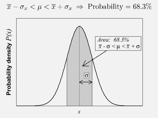
then we can “estimate” whether a certain result is reasonable:

if within $1\sigma_x$, then in general you can say it is good agreement
within $1\sigma \sim 2\sigma$, it is consistent (but probably need more measures)
beyond that it is not very good

note that if the error bar is very large, it does not mean your measurement is automatically good = caveat to mention in your report

Error Propagation

Given some function $f(x,y,z)$, where each variable has uncertainty $x \pm \sigma_x$ etc, then:

\[\sigma_f^2 = \left( \frac{\partial f}{\partial x} \right)^2 \sigma_x^2 + \left( \frac{\partial f}{\partial y} \right)^2 \sigma_y^2 + \left( \frac{\partial f}{\partial z} \right)^2 \sigma_z^2\]

which is valid if the errors on x, y and z are uncorrelated.

Note: you may want to automate this calculation in your python code.

Examples:

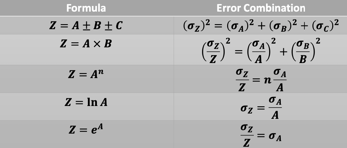
where notice that

relative uncertainty = $1\pm (\sigma_x / \bar{x})$, absolute uncertainty $\sigma_x$
relative uncertainty is useful when you are doing multiplication

Graphical Analysis of Data

When plotting data, you want to show at minimum a) uncertainty = error bars; b) axis labels

But often you would also want to fit a linear model given this data, i.e.

\[y_i = ax_i + b\]

where your measurements are $(x_i, y_i)$. Obviously you will not be able to get a perfect fit, so we consider:

\[\hat{y}_i = ax_i + b\]

and hope to pass as close as possible to the highest number of points = linear regression = minimize least square errors

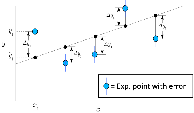
given the error = residuals $\Delta y_i = y_i - \hat{y}_i$, then you consider a

\[\min_\beta J = \min_\beta \frac{1}{2N}\sum_{i=1}^N \left( y_i - \hat{y}_i \right)^2 = \min_\beta \frac{1}{2n}\sum_{i=1}^N \Delta y_i^2\]

where $\beta = (a, b)$ in this example.

the more general case if to of course consider linear algebra formulation
\[\mathbf{y} = \mathbf{X\alpha + \beta} = \mathbf{[1,X] \beta} \equiv \mathbf{X\beta}\]
where $\beta = [\alpha_1, \alpha_2…,\alpha_n, \beta]$. This is so that you can more easily find your least square solution.
one interpretation of why your model is not perfect is to consider how $y$ are constructed. Consider a process where you have a random Gaussian noise to generate those data
\[\mathbf{y} = \mathbf{X\beta} + \epsilon\]
meaning the residuals you have $\Delta y_i = \epsilon_i$, so that if the your model is correct you should see

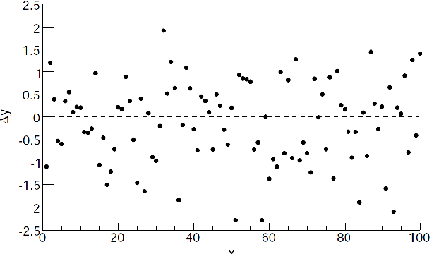
which would be a good way to perform sanity check.

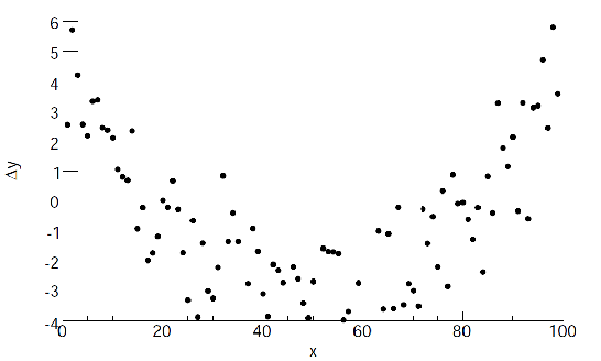
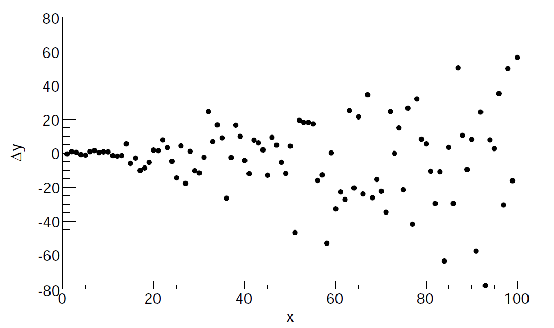
But there are cases when you see that plotting $\Delta y_i$ gives (not limited to only those two cases):

Case 1	Case 2

where:

in case 1 it could be you are fitting a wrong model, or you have some systematic error
in case 2, you might need a some form of a weighted fit

Lab 1

Basically we are re-imagining Galileo’s ramp experiment, where basically we are considering:

motion under constant acceleration
forces will affect the acceleration of a mass (newton’s second law)

The apparatus we will be using is the Fritionless Air-Track

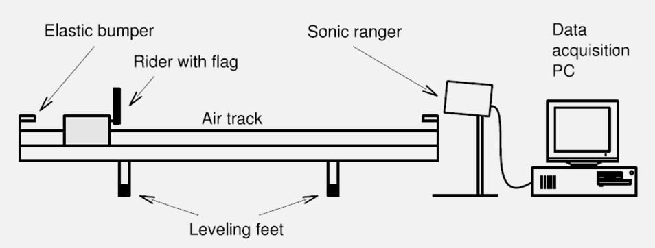
where Timing is performed by Sonic Ranger.

Sonic Ranger: Measuring Velocity: It simply computes the average velocity over very small time intervals

Then, one can then have a measure of the elasticity of a collision by computing the coefficient of restitution

\[e = \left| \frac{v_f}{v_i} \right| = \begin{cases} 1 & \text{elastic}\\ <1 & \text{non elastic} \end{cases}\]

Three main parts

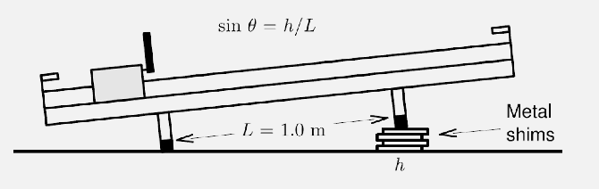
Leveling the ramp
Measuring the elasticity of the bumper (under constant velocity)
- By comparing the velocity before and after, you can compute elasticity (note to propagate uncertainty to compute $e$)
- note that since $e = \vert v_f / v_i\vert$, then the uncertainty is:
  \[\sigma_e^2 = \frac{1}{v_i^2}\sigma_{v_f}^2 + \frac{v_f^2}{v_i^4}\sigma^2_{v_i}\]
- will measurements/error of $v_i$ be dependent on $v_f$? In this experiment, theses two are treated as independent variables so intuitively no. But practically you need to be careful about this.
Measuring the acceleration due to gravity (under constant acceleration
- When you incline the ramp, the size of the gravitational force along the ramp is proportional to the angle of the ramp incline
  
  for which you can estimate acceleration with both $v(t)=a_x t$ and $x(t)=…$.
- then, once you have measured $a_x$, you can compute your $g$ by
  \[a_x = g \sin(\theta) = g\frac{h}{L}\]
- Do you expect steeper slopes to be more accurate than shallower ones? Why or why not?
  - measurement readings error as there is less time when $h$ is high $\implies$ $a_x$ is high $\implies$ less time to collect data $\implies$ more error introduced
  - if there is systematic uncertainty, then relative uncertainty of height becomes less
  - the higher velocity means other contributions such as air resistance becomes more significant
Challenge: estimate friction by looking at the loss of energy

Check: when you doing linear regression for this lab, you are probably going to just do the unweighted version $\implies$ do not need to capture uncertainty

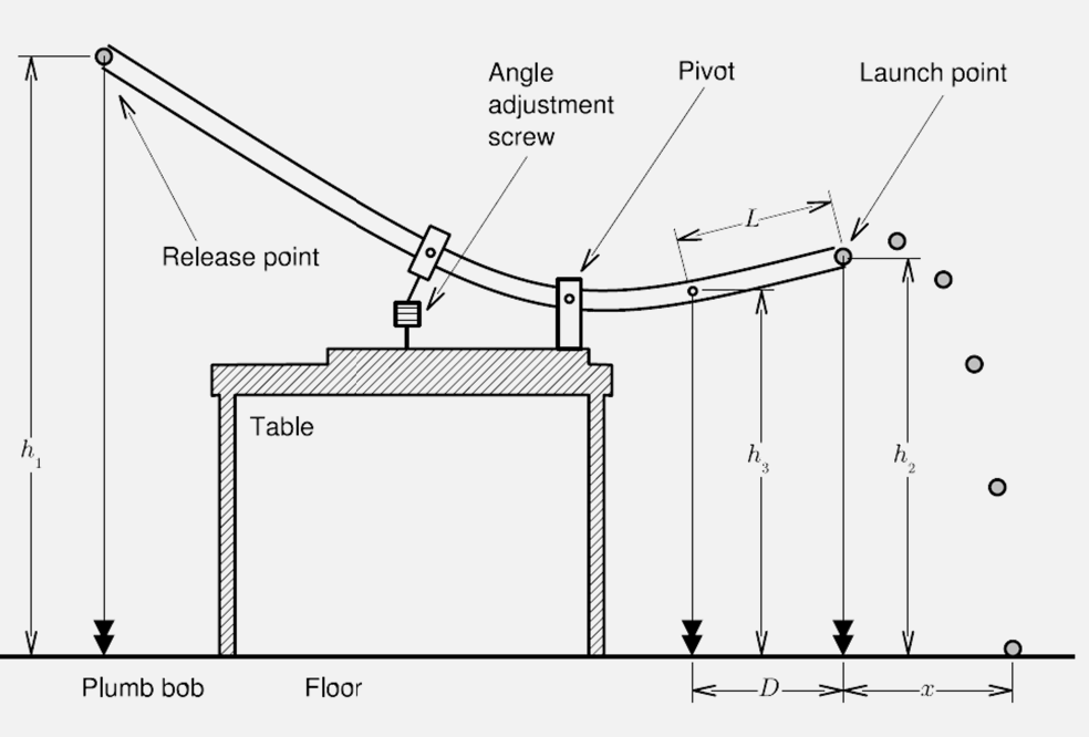
Lab 2: Projectile Motion and Conservation of Energy

Overview: basically launching a ball of a ramp, so that you can

estimate friction
predicting landing position

Primary objectives

understanding distributions of data

Gaussian statistics

write (at least some part) of your derivation in your lab report

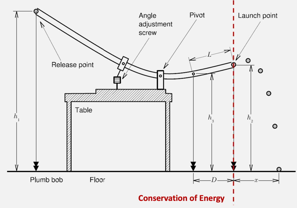
So how does this work? We are essentially exchanging potential and kinetic energy in a closed system

Then, since kinetic energy is

\[E_{k} = \frac{1}{2}mv^2 + \frac{1}{2}I\omega^2\]

for rolling without slipping, $\omega R = v$. and potential energy is

\[E_{p}(r) = -G \frac{M_e m }{r} \approx mgh\]

But of course, often we get energy “leaked” to friction, e.g. $W_f$ work done by friction

\[E_{k}^{ini} = E_k^{fin} + W_f\]

or the canonical form from work-energy theorem

\[W = \frac{1}{2}mv_f^2 - \frac{1}{2}mv_i^2\]

Then, the position of the ejected ball can be described by

\[x(t) = x_0 + v_{x,0}t\\ y(t) = y_0 + v_{y,0}t - \frac{1}{2}gt^2\]

This should summarize all you need. You basically get

$E$
$\Delta E_p = mg \Delta h$
$\Delta E_k = (7/10) m v_0^2$
$W_f = mg \Delta h’$ for $\Delta h’$ being the height at which the ball stops
..blablabla

with which you can find out the final landing position $x(t)$

Note that

the friction force we are estimating is technically velocity dependent. So measuring friction at one configuration might not mean you have the same friction in later setups

The experiment is extremely sensitive to the value of $W_f$, so measure it as carefully as possible!

Taking Data

Basically you will record the position of the landing by having the ball hitting a carbon paper:

draw a marker of where you expect it to land
compare against the actual data

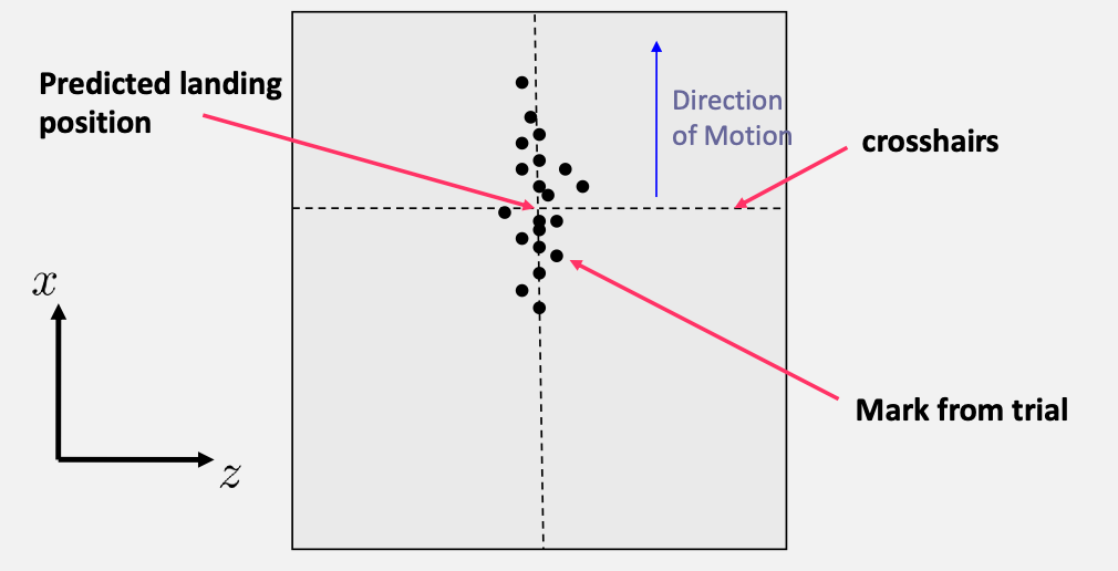
Then, we can look at the distribution of the data

Note

you should expect your data to look like a normal distribution (even if your model is wrong) if you are testing stuff in the same configuration

error propagation in this lab is onerous. It is then highly recommended that you define
\[x_{app} = \frac{D\sqrt{2h_2h_E}}{L};\quad h_E = \frac{10}{7}(\Delta h - \Delta h')\]
$h_2$ and $h_E$ are not independent. Therefore you should really calculate $\sigma_u$ for $u = h_2h_e$

Lab 4

Primary Learning Goals:

Weighted linear regressions
Weighted means of population of data

And we will be probing atomic structures. Before, we understood the classical macroscopic force between matter, but not really what the constituents of matter were

JJ Thomson shows that matter has constituents that are negatively charged and whose charge/mass ratio is constant = quantization!
proposed the plum pudding model (not quite right, improved by latter models)
today, quantum mechanics! Ann the standard model of elementary particles

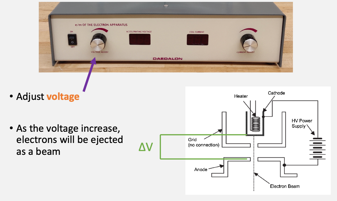
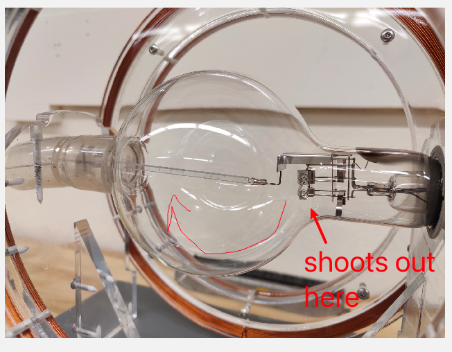
Experiment: measure $e/m$ by using lorentz force giving a circular motion

given a loop current, we can compute the magnetic field created

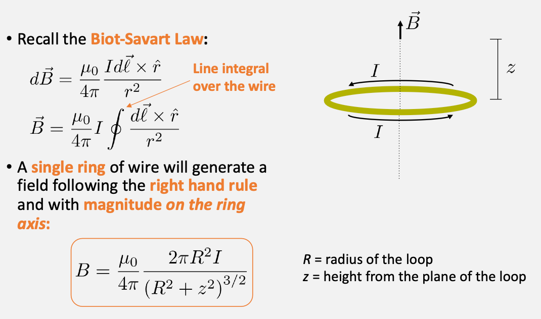
specifically, we will use a Helmholtz coil, which is basically two coils:

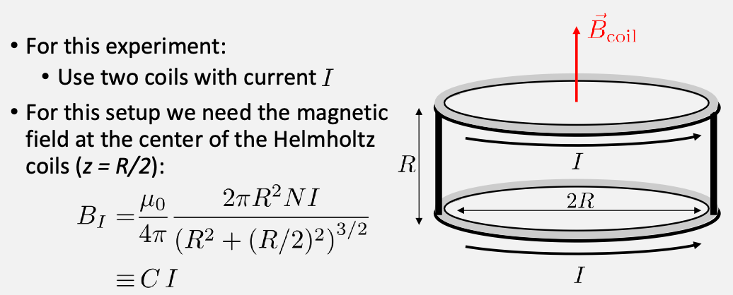
and $C$ will be given.

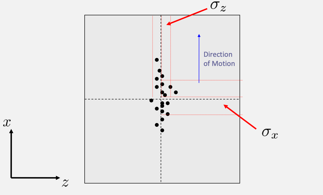
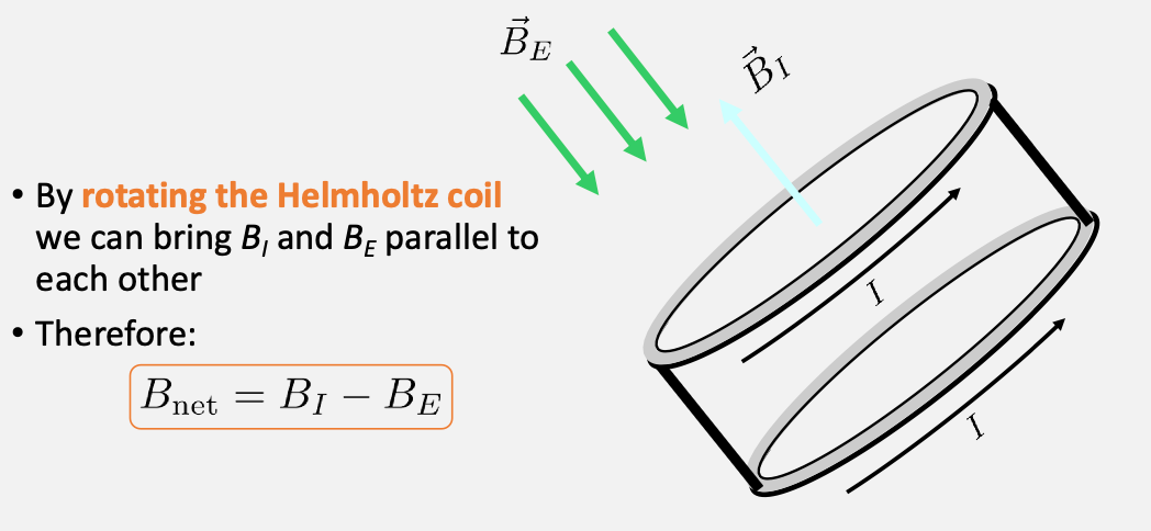
magnetic field at the center of experimental apparatus. Finally we also want to not have contribution from external field, hence you want to align your apparatus with any external field (very important)
Then, in this field (around the axis of the loop) if we send in a moving charge:
\[F = q\vec{v}\times \vec{B} = m \frac{v^2}{R}\]
which performs a circular motion with radius $R$. Hence
\[\frac{q}{m} = \frac{2v}{R^2 B^2}\]
but we don’t have an easy way to measure the velocity $v$. One solution to this problem is to speed the electrons up thanks to a known potential difference
\[K_{\mathrm{gain}} = e V = \frac{1}{2}mv^2\]
assuming $v_0=0$ is at rest and accelerated across $V$.

Spefically:
measure the radius of curvature

Finally, plot with a line of best fit to a equation = shows that the equation is linear hence has more physical meaning (e.g. than computing $e/m$ for each of your trial and averaging across)

note that you will need to pick different $I$, one good way is to pick it such that it hits one of the markers
what about the error of the $I$? You will notice that the marker is quite thick. So you can take $I_\min$ and $I_\max$ that hits that marker, and then take $\bar{I}\pm \sigma_I$ as uncertainty

Lab 5: Polarization and Interference

A few background:

light as EM wave = oscillating E and B fields
Electric and magnetic fields are always perpendicular to each other
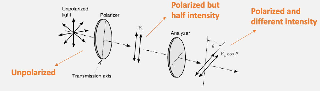
Everyday light is usually unpolarized. All directions of the electric field are equally probable
- a polarized light, e.g. electric fields points in one direction only
- so a better definition/visualization of unpolarized light = cannot define a plane where it oscillates in

Then how much field will be transmitted is given by a linearly polarized light:

\[|\vec{E}_{trans}| = | \vec{E}_0 | \cos\theta\]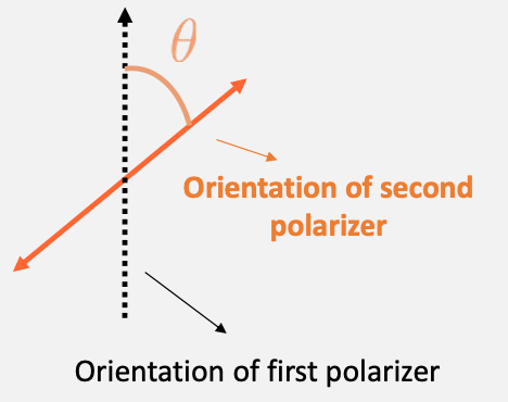

Experiment 1 Background Mauls’ law: but all we care is its intensity because that is what our eyes can observe

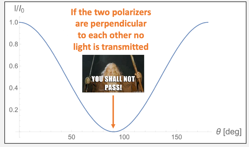
\[I \propto | \vec{E} |^2\]

Therefore we get Malus’ Law (at the second polarizer)

\[I=I_0 \cos^2\theta\]

so you should see something like this

So how do you measure this? You will get a setup with a rotatable polarizer:

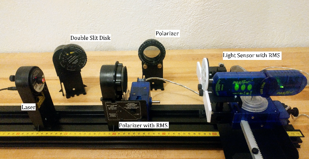
So that you can

Measure this	Plot this

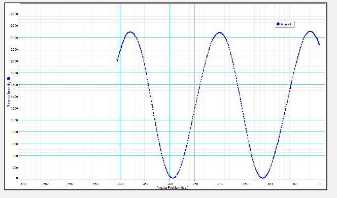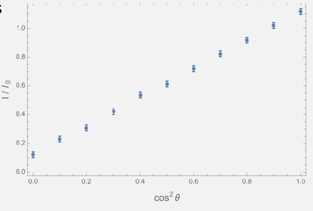where in the plot you will need to extract at least 20 points = 20 different values of $\cos^2\theta$

Experiment 2 Background: Young’s Double Slit

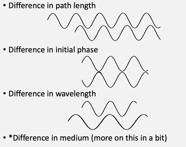
constructive interference = same propagation direction, same frequency, in phase
destructive interference = same propagation direction, same frequency, but out of phase
(recall that standing wave = opposite propagation direction, same frequency)

Here we focus on the constructive and destructive interference

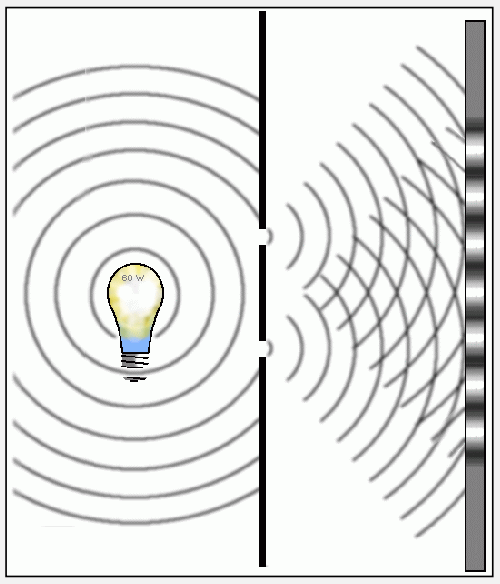
the idea is to measure where the peaks/dark spots are. The key insight is that:

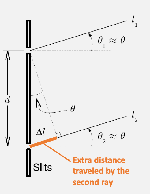
assumption to make thing easier: two waves are parallel, as $D » d$

for bright spot to appear, then the $\Delta l$ must be an integer multiple of wavelength = $m\lambda$
for dark spot to appear, then $\Delta l$ will be $(m+1/2)\lambda$

Then for the positions for the bright spot is

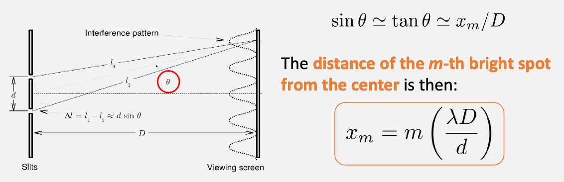
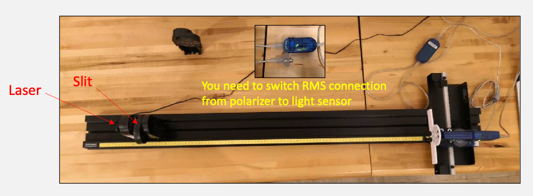
How do you measure this? There will be a sensor you can move along $x$, and record intensity $I(x)$ so that you can find $x_m$

Experiment 3 Background: Diffraction: can be thought of as self-interference:

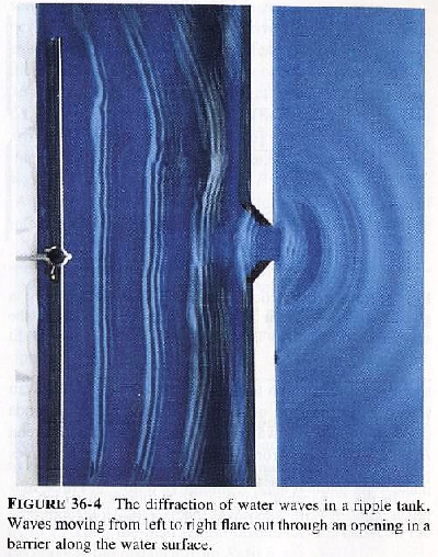
where the diffraction single-slit minima occurs at

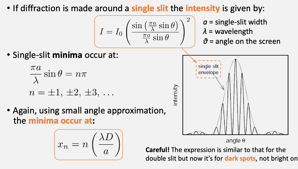
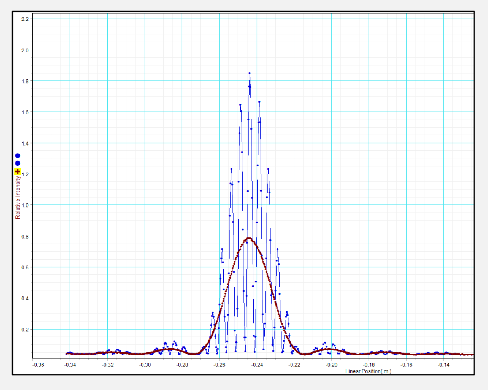
so that you can overlay your single-slit minima envelop on top of your double slit experiment. How did this happen?

in an ideal double slit, all the amplitudes will be constant. In an “ideal” single split, you get your envelope
therefore in the practical double split, the observed intensity is actually an ideal double split $\times$ single slit

How would yuo measure this? Once again take measurements by moving the sensor in the transverse direction

What are some questions to think about:

What limits the precision of these measurements with light? theory, physical limitations, aberration, diffraction, ambient lights

Some tips:

For all the three parts: Move the RMS slowly when recording data.
For the polarizer part: Try your best to minimize the amount of environmental light coming in. E.g. using the dim light in the room, move components closer to the sensor, etc.
For the last part: move the laser closer to the light sensor to see more fringes but remember to record the value of D!

Lab 6: Interferometer

The idea that we can use light as a precision measurement tool. Recall that some key properties include

interference

basically when two waves interfere under different conditions
refraction, governed by snell’s law

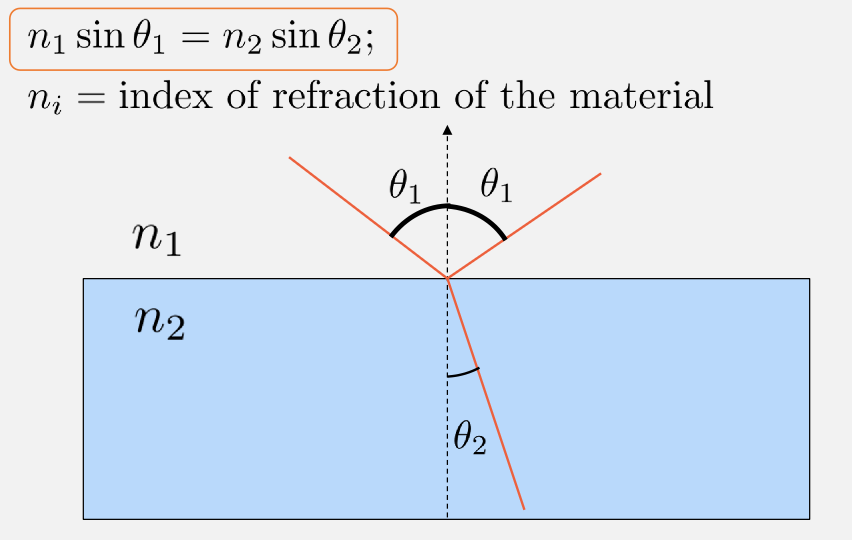
so that basically, as Maxwell’s equation is “different” in medium, we get
\[v = c/n,\quad n \text{ being index of refraction}\]
optical path length: how many “cycles” the light spend during the a physical distance

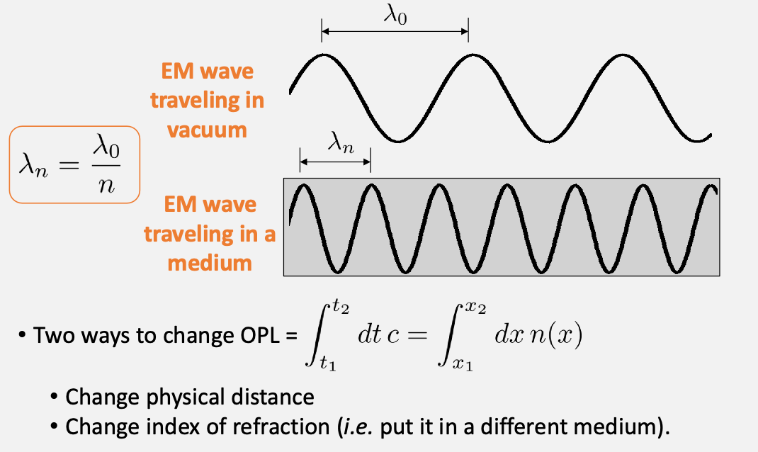
in the case of different medium (but same physical distance), then you can simply calculate the number of wavelength we can fit in each “box” (i.e. physical distance)

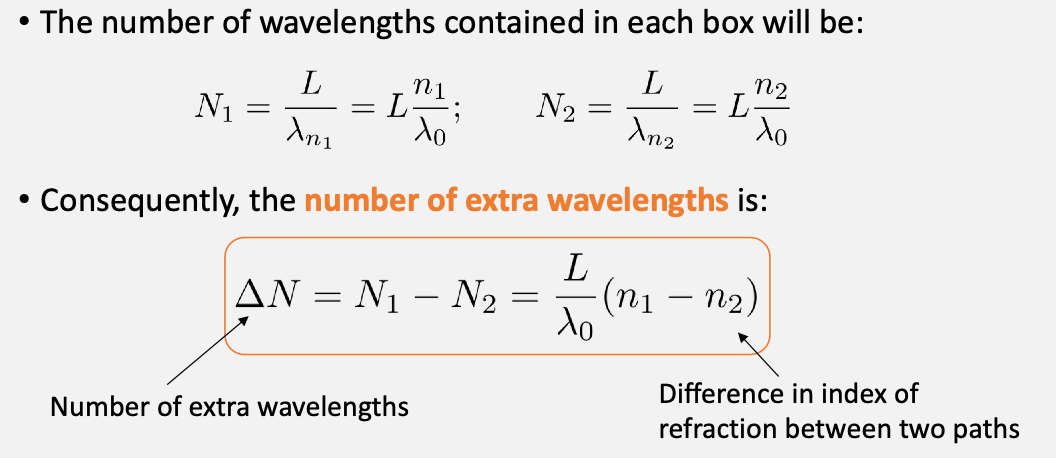
why would this quantity be useful? Recall that in the previous lab this difference in wavelength relates to constructive/destructive interf.

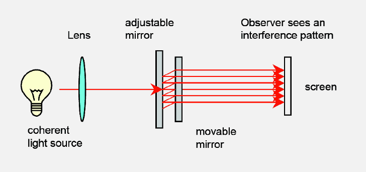
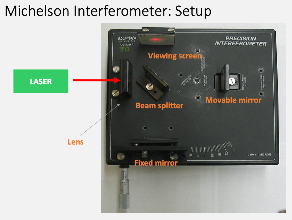
Finally, interferometry, the idea being

Split single beam into two, then recombine.
Observer sees interference patterns projected onto a small screen.
By moving one of the mirrors, the observer can change the path length difference . The consequence is a shift in the interference pattern.

so that as you move the $M_1$ length back and forth, you will see a different interference pattern

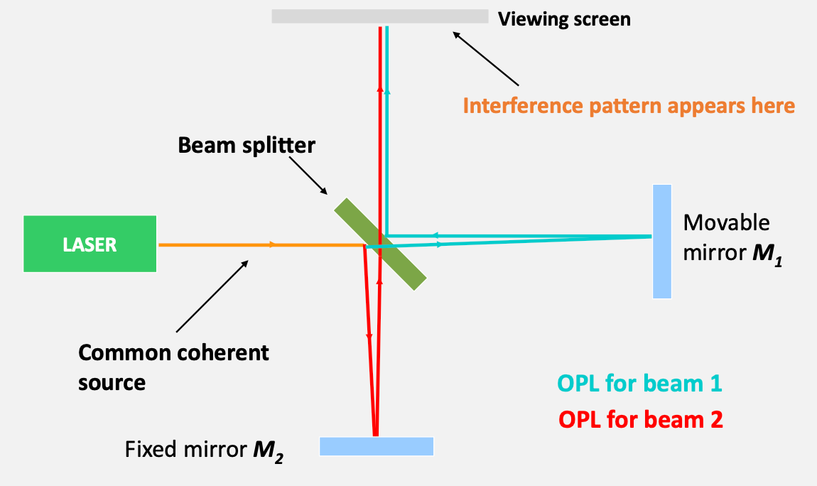
where basically you get two rays because one is being transmitted and other being reflected

measure the gravitational wave=stretching/compressing space=changes the physical distance=interference pattern

Inteferometers Today	Recorded Interference due to Gravitational Wave

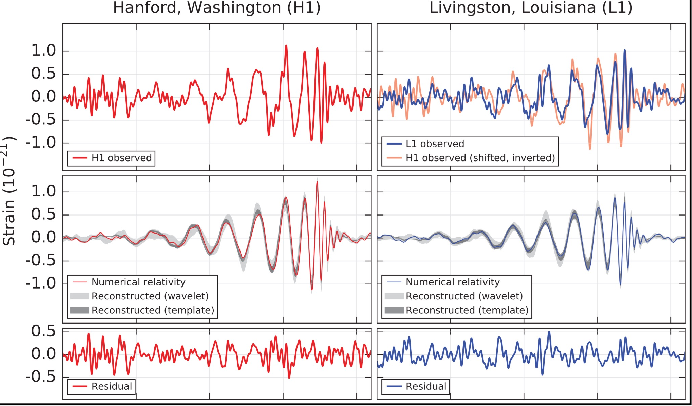Alternatively, the beams that are transmitted and reflected+transmitted will have interference = can measure the gap

If we change the path length by a certain distance
\[2d_m = m \lambda,\]
where $d$ is the distance you moved the mirror w.r.t the original position, then you will restore the original intereference pattern.

be careful that the drawings we did are “assuming” a single light ray, but of course in reality is a “spherical wave front”

therefore, if you moved $d_{10}$, then you would have seen the bright spot reappeared $10$ times during the time you moved it

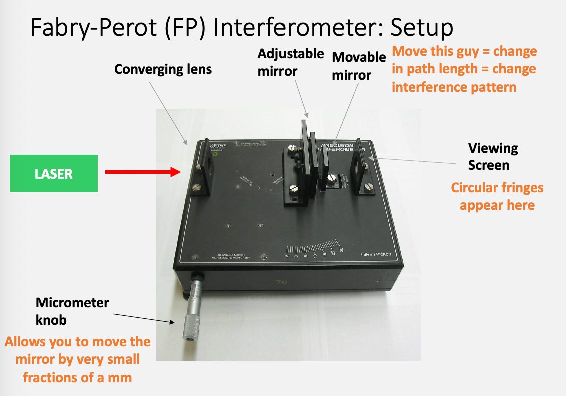
Experiment: you will use both the Michelson and the Fabry-Perot interferometers

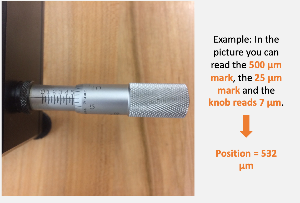
How to read the micrometers

You will turn the knob and count how many fringes have passed.

Then you will do this again:

To think about:

in the end both setup measures the same thing. Which configuration is better?

sometimes count the first fringe might be hard. It could be better to count the second ring, etc = the largest error is most likely mis-counting the number of fringes. So that should be included in your uncertainty measurement

The last part is we can change the optical distance by changing the medium (before we are changing the physical distance)

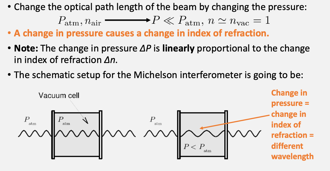
so that we can change the pressure=change index of refraction and observe different interference patterns.

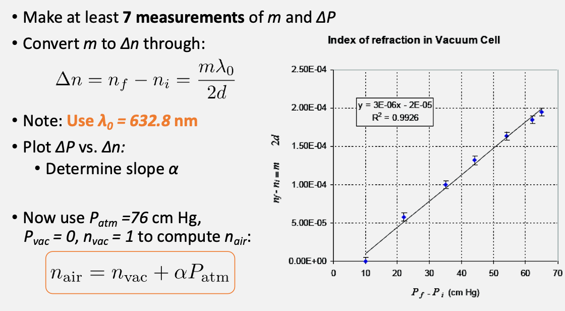
Therefore, since the interference patterns re-occur every integer number of wavelengths apart:

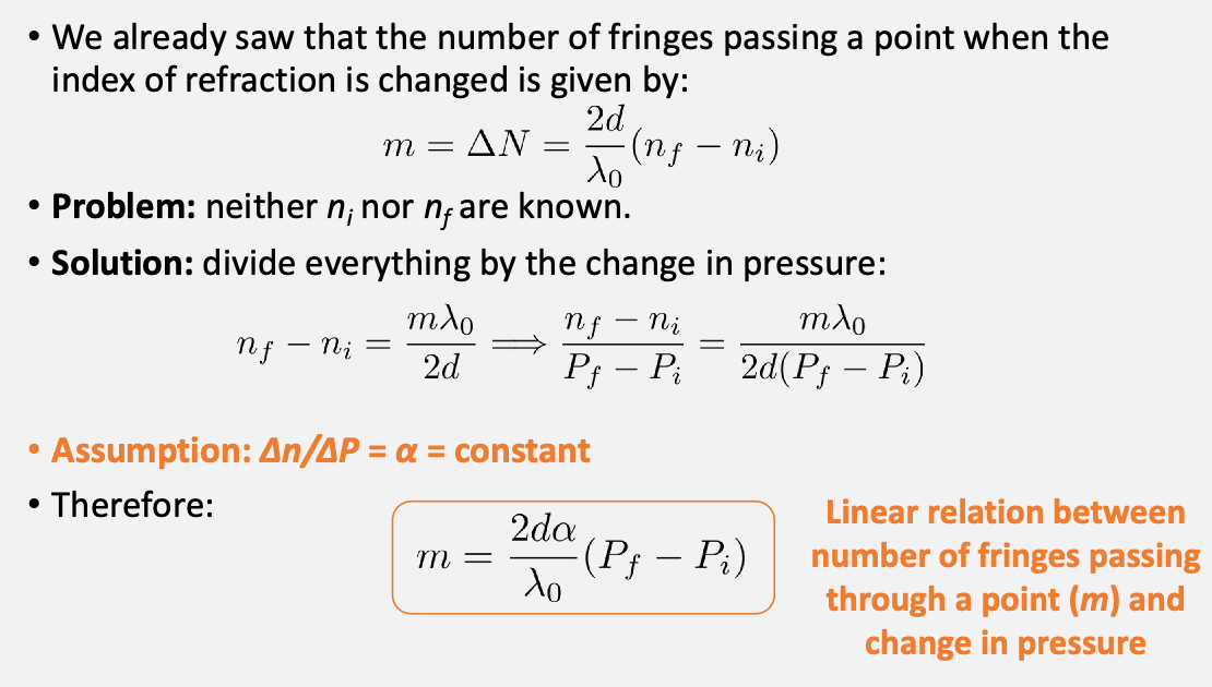
Then finally from this we can compute $n_{air}$ by

Tips

start turning the knob from the 500 $\mu m$ mark

Feedback Received

Feedback for Lab 1:

Total score: 13.5/20

Overall Communication/Organization rubric items: Full points

Data Vis: -1 Plots must have titles as well as captions. Note: A short table or two with some of your measurements would not have been out of place here, but it’s not strictly necessary and in this case, you wouldn’t lose points

Data Manipulation & Error Analysis rubric items: -1 - Uses Python, Mathematica, or similar: Yes - Only most relevant equations or analyses are explicitly shown: Yes - Analysis and modeling are connected to physical concepts: Yes - Uncertainties are justified: There is no such thing as “human error.” This will fall under “random error” but never use the phrase “human error” or anything like it.

Discussion rubric items: -3.5 - Comparison of results to expectation with justification: Agreement of measured e with expected value (1) is not reported. When discussing whether results are in agreement with predictions, don’t say that your results are “satisfactory” or “close” or anything like that (e.g. when you talked about your result for b, the y-intercept). When it comes to analyzing results, there’s only one thing that matters. Are your measurements the same as the predicted values within 3 sigma? If yes, they’re in agreement with predictions. If not, there’s a statistically significant error and they’re not in agreement. Once you have established this, you go into discussing the quality of your results (why they were or weren’t in agreement), and then you can potentially use more qualitative descriptions, but only once the quantitative actual analysis has been established. - Discussion of quality (quantitative and qualitative) of results: Whether or not your results are in agreement with expectation, need to comment on why. This hasn’t been done fully. - Sources of errors reference model, assumptions, and technical limitations: Sources of error for e not commented on. - Responds to discussion questions: Not all

Narrative flow & context rubric items: -1 - Sufficiently contextualize results and discussion: Yes - Include only necessary and relevant background: Yes. If you want it to be perfect, you need to include just one or two sentences that capture the really big picture (why do we even care about any of the things we investigated in this experiment). You’re really almost there, but think of the intro as the part that will convince the reader that this is worth reading. Think of a scientific journal article where the intro always has something to make the project sound immediately relevant to everyone, no matter their background. - Separate information appropriately: Yes - Summarize concisely: Yes