CSOR4231 Analysis of Algorithms
- Analysis of Algorithms
- Introduction
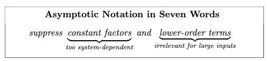
- Asymptotic Notation
- The Master Method
- Linear-Time Selection
- QuickSort
- Graphs: The Basics
- Dijkstra’s Shortest Path Algorithm
- Hash Tables and Bloom Filters
- Introduction to Greedy Algorithms
- Huffman Codes
- Prefix-Free Codes
- Huffman’s Greedy Algorithm
- Correctness of Huffman’s Algorithm
- inductive step: we need to show that $P(k)$ is true. Since each step of the algorithm we are merging two least frequent “symbols” (the root of the subtree), we want to show claim 1 and claim 2 to hold in order to prove that the output tree at this stage is optimal.
- Running Time of Huffman Algorithm
- Minimum Spanning Trees
- Introduction to Dynamic Programming
- Advanced Dynamic Programming
- Shortest Path Revisited
- Max Flows and Min Cuts
- Linear Programming
*Picture credits from the Algorithms Illuminated book
Analysis of Algorithms
Logistics: Mostly see Canvas, but just note that:
- 10 Psets, no late days, but 2 can be dropped. Each pset worth 10 points.
- 3 non-cumulative exam, each worth 60 points. Tentative dates Oct 3, Oct 31, Dec 7.
- exams will have about 50% content verbatim from HW
- textbook: the split version of Algorithms Illuminated will have the same content as the Algorithms Illuminated Omnibus version, except that problem numbering might be different
- skim the readings before/after class, as they are the content you are responsible for
Example demo algorithmic questions:
*For example*: Routing in Internet. Let nodes/vertices be hosts, and edges be the physical/wireless connections. Let the connections be bidirectional. How do you figure out the shortest path (least number of hops) between two given hosts?
-
Dikstra algorithm: given a source host (e.g. node 0), we can find the shortest path to all other hosts. The key insight shortest path is composed of shortest path, assuming all edges are positive. This means that if you have a given shortest path from $v$ to $u$, and nodes $w,x,y,z$ are only connected to $u$, then any shortest path from $v$ to $w,x,y,z$ must go through $u$.
The algorithm iteratively grows a “tree” of visited nodes. At each iteration, the node that has the smallest cost (e.g. node 1) will be marked as done. THen we add all the neighbors of that marked node (because of the insight above) to the tree of visited nodes, and update the cost of the neighbors.
however, the issue is that it needs to remember information about the entire internet during computation (i.e. keep an adjacency matrix/is visited of all nodes), which is not scalable.
-
Bellman-Ford algorithm: a differential version that converges to the shortest path.
*For example*: Sequence alignment. Consider two strings composed of characters ${ A,C,G,T }$:
\[AGGGCT, AGGCA\]How similar (smallest edit distance, or lowest NW score) are the two strings?
- Brute force: try all possible alignments, and pick the one with the lowest score. Insanely expensive.
- Dynamic programming!
*For example:* Multiplying two numbers. Given two $n$ digit number (e.g. $x=1234$, $y=5678$), find a way to find out their product.
-
Grade school approach: multiply each digit by each, get partial product, and sum.
Cost is $O(n^2)$ as for each digit need to do $n$ multiplication, and there are $n$ digits
-
Recursive v1: We can break down multiplying numbers into multiplying parts of it and add back (divide and conquer). For instance, let $x=10^{n/2}a + b$ and $y=10^{n/2}c + d$ (e.g. $a=12, b=34$ for $x=1234$). Then realize that:
\[\begin{align*} x\cdot y &= (10^{n/2}a + b) (10^{n/2}c + d) \\ &= 10^n ac + 10^{n/2} (ad + bc) + bd \\ \end{align*}\]and then, for each of the 4 multiplication operation, we can further recurse into smaller components until we are at one digit.
Is this necessarily faster than grade school? We will analyze this in the course.
-
Recursive v2 (Karatsuba Algorithm): An improved version than above where we only do 3 multiplications instead of 4. Notice that we can rewrite:
\[(a+b)(c+d) = ac + ad + bc + bd = ac + bd + (ad + bc)\]therefore, to equivalently compute the 4 multiplications in v1, we can do:
- compute $ac$
- compute $bd$
-
compute $(a+b)(c+d)$ and subtract $ac$ and $bd$ from it to get $ad+bc$
Introduction
The basic idea is to break your problem into smaller subproblems, solve the subproblems (often recursively), and finally combine the solutions to the subproblems into one for the original problem.
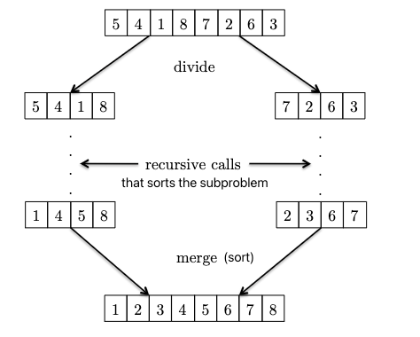
MergeSort: The Algorithm
MergeSort is a classical sorting algorithm using the divide and conquer paradigm. Recall that to sort an array, we could have done:
SelectionSort: scan the array, find the smallest element, put it in the first position, and repeat.InsertionSort: keep two arrays, sorted and unsorted. Scan the unsorted array and place the smallest element there into the correct position of the sorted array.BubbleSort: swap adjacent elements to make sure the smallest is in the first position, then repeat.
the above three simple algorithms have a running time of $O(n^2)$, which is not great. We can do better with MergeSort. High level idea:
where:
- given two sorted subparts, we can combine them into a sorted array by
mergingthem (use a pointer at each of the two subpart, and just move the smallest element of the two to the output array). You will see after the Master Method that the key to $O(n \log n)$ is that this merge only takes $O(n)$!. - from the above you see the recursive nature: the base case of just one element is already sorted! So we can use this base case AND the above merging operation to sort the entire array.
Specifically, the pseduocode is:
# input: array A of n distinct numbers
# output: return a sorted array from smallest to largest
def merge_sort(A):
	# base case
	if len(A) == 1:
		return A
	c = merge_sort(A[:n//2])  # recursively sort the first half of A
	d = merge_sort(A[n//2:])  # recursively sort the second half of A
	return merge(c, d)
so basically all the work is to merge the two sorted subarrays into one sorted array. The pseudocode for merge is:
def merge(c, d):
  i = 1
  j = 1
  e = []
  for k in range(len(c) + len(d)):
    # there is a bit more code to deal with if one of the two arrays is exhausted
    # if the first unused element from c is smaller, then add it to e
    if c[i] < d[j]:
      e.append(c[i])
      i += 1
    # otherwise, add the first unused element from d to e
    else:
      e.append(d[j])
      j += 1
  return e
So what is its runtime? How fast is this compared to $O(n^{2})$?
MergeSort: The Analysis
On a high level, we can imagine the runtime as “the total number of lines of code/operation we need to execute to run the implementation”. How do we approach this? In general, we should first visualize what the algorithm does.
For recursive algorithms such as MergeSort, we can visualize it as a recursion tree:
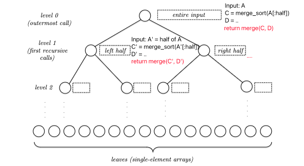
so basically, at each node THE REAL COST is merge(C,D), assuming your code implementation can slice arrays in halves using $O(1)$ time. This means that the total runtime is:
For a recursive algorithm, generally notice that each level will receive similar input (e.g. sizes). Therefore, we can instead consider:
\[\sum_{j \in \text{all levels}} \text{(\# of nodes at level $j$)} \times \text{(Cost of merge(C,D) at level $j$)}\]Hence we get, for an input of length $n$ (assuming its a power of $2$)
- in total there are $\log_{2} n + 1$ levels
- at each level, there are $2^{j}$ nodes (note that you can imagine growing a tree from top to bottom as an exponential operation, while collapsing it from bottom to top as a logarithmic operation)
- the input size at each node would therefore be $n/2^{j}$
- the cost of
mergeat a node (using the pseudocode above it is about $4m+2$, where we have $4$ operations during the loop and 2 initialization operations). For simplicity let it be $6m$.
The total cost at each level is therefore:
\[2^{j} \cdot 6 \left( \frac{n}{2^{j}} \right) = 6n\]and finally the total runtime cost is:
\[\sum_{j \in \text{all levels}} 6n = \left( \log_{2} n + 1 \right) \cdot 6n = 6n \log_{2} n + 6n = O(n \log n)\]Important notes:
- here we considered the worst case scenario. This would be appropriate for general purpose algorithms as we won’t know what the input is.
- What about “average-case analysis”? For example, in the sorting problem, we could assume that all input arrays are equally likely and then study the average running time of different sorting algorithms. A second alternative is to look only at the performance of an algorithm on a small collection of “benchmark instances” that are thought to be representative of “typical” or “real-world” inputs.
- we are sloppy for constant factors/coefficients. This is because:
- in real life these constants will be heavily implementation dependent
- will see how the Big O notation will not care about these constants
- related to above, we will focus on how runtime scales with input size $n$. Especially when $n$ become large.
- yes, there are cases when a runtime of $0.5n^{2}$ is faster than $6n \log n$, for example when $n=2$. But smart algorithms doesn’t really matter if $n$ is small!
- the holy grail is a linear-time algorithm (seeing each input ~once). For some problems we will not find a linear time algorithm, and for some (e.g. binary search) we can by “cheating” (we are already given an sorted array)
Strassen’s Matrix Multiplication Algorithm
This section applies the divide-and-conquer algorithm design paradigm to the problem of multiplying matrices, culminating in Strassen’s amazing subcubic-time matrix multiplication algorithm.
Recall that matrix multiplication considers
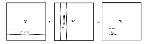
Therefore the very basic algorithm would be:
def matrix_mut(X, Y):
  # X is n x n, Y is n x n
  for i in range(n):
    for j in range(n):
      Z[i][j] = 0
      for k in range(n):
        Z[i][j] += X[i][k] * Y[k][j]
  return Z
which is obviously $\Theta(n^{3})$
Since the input size is $O(n^{2})$, the best we can hope for would be $O(n^{2})$ runtime. So can we do better? Emboldened by the divide and conquer integer multiplication algorithm, we can try to divide the matrix into smaller submatrices and then recursively compute the product of these submatrices.
Consider breaking the matrix down to:
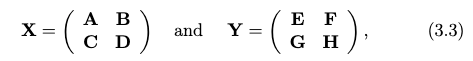
then we can write the product as:
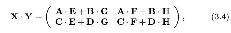
where adding two matrices is just element-wise addition with cost $O(l^{2})$ for $l \times l$ matrices. Therefore, analogous to the integer multiplication algorithm, we can write the matrix multiplication algorithm
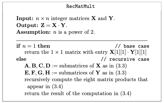
which has basically eight recursive calls. The problem is that this is still $\Theta(n^{3})$!
The key insight from the Karatsuba algorithm was that we can save one multiplication by using some tricks, and that can help us get sub-cubic time!
A high level description looks like:
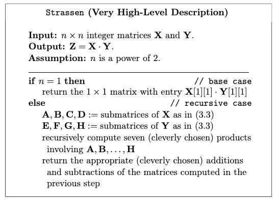
Details of Strassen’s Algorithm
The key detail is how to save the extra multiplication. The idea is to use the following 7 auxiliary matrices:
which involves $O(n^{2})$ time doing additional matrix additions, but just with these seven we can compute the matrix product as:
which works due to some crazy cancellation, for example in the upper left:
the rest you can check yourself, but with it down to 7 recursive calls, we can compute the runtime (using the The Master Method): $O(n^{2.807})$!
Asymptotic Notation
The high level idea of why to use Big O:
where saving one recursive call is a bigh win, because that will get saved over and over again as the recursion goes deeper.
Big-O Notation
Let $T(n)$ denote the worst-case running time of an algorithm we care about, where $n={1,2,3, …}$ being the size of the input. What does it mean to say something runs in $O(f(n))$ for some function $f(n)$?
Big-O Notation: $T(n) = O(f(n))$ if and only if there exist positive constant $c$ and $n_0$ such that:
\[T(n) \leq c \cdot f(n),\quad \text{ for all } n \geq n_0\]i.e. eventually when input gets large enough, $T(n)$ is bounded by $c \cdot f(n)$. So all you need to show/prove is that you can construct a $c$ and $n_0$ such that it holds.
Pictorially, we can imagine:
For Example: a degree-$k$ polynomials are $O(n^{k})$. Suppose:
\[T(n) = a_{k} n^{k} + a_{k-1} n^{k-1} + ... + a_{1} n + a_{0}\]for $k \ge 0$ and $a_i$’s are real numbers. We can show that $T(n) = O(n^{k})$:
\[\begin{align*} T(n) &= a_{k} n^{k} + a_{k-1} n^{k-1} + ... + a_{1} n + a_{0} \\ &\le \left|a_k\right| n^{k} + \left|a_{k-1}\right| n^{k-1} + ... + \left|a_{1}\right| n + \left|a_{0}\right|\\ &\le \left|a_k\right| n^{k} + \left|a_{k-1}\right| n^{k} + ... + \left|a_{1}\right| n^k + \left|a_{0}\right| n^k\\ &= \left(\left|a_k\right| + \left|a_{k-1}\right| + ... + \left|a_{1}\right| + \left|a_{0}\right|\right) n^k\\ &\equiv c \cdot n^k \end{align*}\]holds for all $n$, so $n_{0} = 1$ and $c = \left\vert a_k\right\vert + \left\vert a_{k-1}\right\vert + … + \left\vert a_{1}\right\vert + \left\vert a_{0}\right\vert$.
For Example: a degree-$k$ polynomial is not $O(n^{k-1})$. Suppose for simplicity $T(n) = n^{k}$. Then proof by contradition that this means:
\[n^{k} \le c \cdot n^{k-1}, \quad \text{ for all } n \ge n_0\]this means:
\[n \le c, \quad \text{ for all } n \ge n_0\]which is a contradiction as $n$ can be arbitrarily large.
Big-Omega and Big-Theta Notation
On a high level, if big-O is analogous to “less than or equal to ($\le$),” then big-omega and big-theta are analogous to “greater than or equal to ($\ge$),” and “equal to (=).”
Big-Omega Notation: $T(n) = \Omega(f(n))$ if and only if there exist positive constant $c$ and $n_0$ such that:
\[T(n) \geq c \cdot f(n),\quad \text{ for all } n \geq n_0\]i.e. eventually when input gets large enough, $T(n)$ is bounded below by $c \cdot f(n)$.
Pictorially, bounding from below means:
and we would call $T(n) = \Omega(f(n))$.
Big-Theta Notation: $T(n) = \Theta(f(n))$ if and only if there exist positive constant $c_1, c_2$ and $n_0$ such that:
\[c_1 \cdot f(n) \leq T(n) \leq c_2 \cdot f(n),\quad \text{ for all } n \geq n_0\]i.e. eventually when input gets large enough, $T(n)$ is sandwiched by $c_1 \cdot f(n)$ and $c_2 \cdot f(n)$. Notice that this is analogous to say that both $T(n) = \Theta(f(n))$ and $T(n) = O(f(n))$.
For example, if $T(n) = \frac{1}{2} n^{2} + 3n$, then $T(n) = \Theta(n^{2})$.
Little-O Notation: $T(n) = o(f(n))$ if and only if for every positive constant $c>0$ there exists a constant $n_0$ such that:
\[T(n) \le c \cdot f(n),\quad \text{ for all } n \geq n_0\]i.e. eventually when input gets large enough, $T(n)$ is bounded above by $c \cdot f(n)$ for any $c$ you pick (note that you can pick $n_0$ based on $c$). Also note that this is much stronger than the Big O notation.
Intuitively, this is like saying we want:
\[\lim\limits_{n \to \infty} \frac{f(n)}{T(n)} = 0\]that $f(n)$ grows strictly faster than $T(n)$ (i.e. pick $c$ to be infinitesimally small in the above definition). Also note that the intutive way of converting between Big O and Little O is NOT just switching $\le$ to $<$, as that would actually not change anything (see HW1 Problem 2.7)
For example, $n^{k-1} = o(n^{k})$ is true for any $k \ge 1$.
The Master Method
This “master method” applies to analyzing most of the divide-and-conquer algorithms you’ll ever see, as their runtime typically follows a pattern of the form:
\[T(n) = \underbrace{a \cdot T\left(\frac{n}{b}\right)}_{\text{word done by recursive calls}} + \underbrace{O(n^{d})}_{\text{clean up}}\]where $a$ would be the number of recursive calls you make, $b$ would be by how much you shrink the input size, and $O(n^{d})$ would be the time it takes to combine/clean up any of results of the recursive calls (e.g. the cost for merge in merge_sort).
For Example, recall the multiplication problem. Grade-school algorithm would give us $O(n^{2})$. However,
-
the recursive algorithm v1 (calculate $10^{n}ac + 10^{n / 2}(ad + bc) + bd$) would then give us:
\[T(n) \le 4T(n / 2) + O(n)\]where $4$ comes from doing 4 more multiplications to calculate $ac, ad, bc, bd$, and $n / 2$ because we are chopping each original interger into half $x = 10^{n / 2}a + b$ and $y = 10^{n / 2}c + d$.
-
the recursive algorithm v2 (Karatsuba Algorithm) saves the computation of $ad + bc$ by computing only $(a+b)(c+d)$ and then minus $(ac + bd)$ which would be already computed. Given that addition is done in linear time:
\[T(n) \le 3T(n / 2) + O(n)\]where now you only have to do 3 more multiplications to calculate $ac, bd, (a+b)(c+d)$, with extra work in addition but that is already in $O(n)$ term.
and that for all the above cases, the base case is $T(1) = O(1)$.
Formal Statement
We’ll discuss a version of the master method that handles what we’ll call “standard recurrences”, which have three free parameters and the following form:
Standard Recurrence Format. Let $T(n) = \mathrm{constant}$ for some small enough $n$ (i.e. base case). Then for large values of $n$, we have the runtime being:
\[T(n) \le a \cdot T\left(\frac{n}{b}\right) + O(n^{d})\]where:
- $a$ is the number of recursive calls you make
- $b$ is by how much you shrink the input size
- $O(n^{d})$ is the time it takes to combine/clean up any of results of the recursive calls
Then, we have the master method:
Master Method. If $T(n)$ is defined by a standard recurrence of the form above with $a \ge 1, b > 1$ and $d \ge 0$, then:
\[T(n) = \begin{cases} O(n^{d} \log n) & \text{if } a = b^{d} \\ O(n^{d}) & \text{if } a < b^{d} \\ O(n^{\log_{b} a}) & \text{if } a > b^{d} \end{cases}\]note that
- intuitively, the second one indicates that your algorithm is “clean up step heavy”, and the third one indicates that your algorithm is “recursive call heavy”
- the last case specifically specified a base $b$, whereas the first case did not. This is because any two logarithm base differ by a constant multiple. This will be harmless in the first case because we are multiplying by a constant factor of $d$, but not in the last case because we are raising to a power of $n$.
First for a sanity check, the merge sort algorithm takes the form of:
\[T(n) = 2T\left(\frac{n}{2}\right) + O(n)\]hence we have $a = 2, b = 2, d = 1$, and so $a = b^{d}$, which means that the first case applies and we have $T(n) = O(n^{d} \log n) = O(n \log n)$.
Then we first answer the questions of runtime for KaraSuba algorithm and the recursive algo v1:
- multiplication algo v1 has $a=4, b=2, d=1$ so $a > b^{d}$, hence we have $T(n) = O(n^{\log_{b} a}) = O(n^{2})$, actually just as good as the grade-school algorithm.
- KaraSuba algo has $a=3, b=2, d=1$ so $a > b^{d}$, but we have $T(n) = O(n^{\log_{b} a}) = O(n^{\log_{2} 3}) \approx O(n^{1.59})$, which is better than the grade-school algorithm.
- Matrix Multiplication v1 (splitting into 8 smaller matrix multiplications) have still $O(n^{3})$. To see this, there are two ways: 1) consider $T(n^{2})=8 T(n^{2} / 4) + O(n^{2})$, substitute $n^{2}=u$ we get runtime is $O(u^{\log_{a} b})$; 2) just consider the input $n^{2}$ as a function of $n$, hence runtime is $T(n) = 8T(n / 2) + O(n)$, which gives $O(n^{\log_{a} b})$.
Proof of Master Method
Next we prove the master’s method.
Proof: Suppose that $T(1) = \text{constant}$ and we have the standard recurrence for $n > 1$:
\[T(n) \le a \cdot T\left(\frac{n}{b}\right) + c \cdot n^d\]where we replaced $O(n^{d})$ with $c \cdot n^{d}$ for some constant $c$.
We can try to write a few terms out and see if we can find a pattern, but alternatively we can also draw a recursion tree and see if we can directly find a closed-form equation:
Our goal is to find the runtime of this entire tree. So we consider:
\[T(n) = \sum_{j \in \mathrm{level}} \sum \mathrm{cost}(\text{each node})\]from which we know that:
- there are $a^{j}$ subproblems/nodes at depth $j$
- each node at depth $j$ needs to solve problem with input size $n / b^{j}$
again, assuming splitting the input to $b$ subproblems takes constant time, we have the cost at each node being:
\[\mathrm{cost}(\text{each node}) = c \cdot \left( \frac{n}{b^j} \right)^d\]since at each node it is just the clean up step $c \cdot n^{d}$. Then since there are $a^{j}$ nodes at level $j$, we have:
\[\begin{align*} T(n) &= \sum_{j=0}^{\log_b a} a^j \cdot c \cdot \left( \frac{n}{b^j} \right)^d \\ &= c \cdot n^d \cdot \sum_{j=0}^{\log_b a} \underbrace{\left( \frac{a}{b^d} \right)^j}_{\text{this ratio!}} \\ \end{align*}\]where the ratio of $a / b^{d}$ was the ratio we had in the master method. This ratio also has a very important interpretation:
- $a$ is the rate of growth/proliferation
- $b^{d}$ is the rate of shrinkage of work. Since each of your subproblem shrink by a factor of $b$, but that goes into the term $O(n^{d})$, hence you shrink your work by a factor of $b^{d}$.
Then we have the following cases:
-
if $a = b^{d}$, then:
\[T(n) = c \cdot n^d \cdot \sum_{j=0}^{\log_b a} \left( \frac{a}{b^d} \right)^j = c \cdot n^d \cdot \sum_{j=0}^{\log_b a} 1 = c \cdot n^d \cdot (\log_b a + 1) = O(n^d \log n)\]note that we changed the base here.
-
if $a / b^{d} = r \neq 1$, then we have a finite geometric series where:
\[\sum\limits_{j=0}^{k} r^{j} = 1 + r + r^{2} + \cdots + r^{k} = \frac{r^{k+1} - 1}{r - 1}\]which means that:
-
if $r < 1$, then the first term $O(1)$ dominates. Hence we get
\[T(n) = c \cdot n^d \cdot O(1) = O(n^d)\]which is basically the work done by the root node!
-
if $r > 1$, then the last term $O(r^{k})$ dominates. Hence we get
\[T(n) = c \cdot n^d \cdot O\left[ \left( \frac{a}{b^{d}} \right)^{\log_{b} n} \right]\]note that since $b^{-d \log_{b} n} = (b^{\log_b n})^{-d} = n^{-d}$, we get:
\[T(n) = O(a^{\log_{b} n}) = O(n^{\log_{b} a})\]where $a^{\log_{b} n}$ is basically the number of leaves! However we still use the $n^{\log_{b} a}$ because it’s easier to apply.
-
Linear-Time Selection
This section discusses another divide-and-conquer algorithm, but won’t take the standard form of the master method (probably the only case in this course).
Selection Problem. Given an array $A$ of $n$ distinct numbers and an index $i$, find the $i$th smallest element of $A$.
The naive solution would be a sort + indexing, which takes $O(n \log n)$ time. However, we can do better by using the divide-and-conquer strategy. The intuition is that we can select a pivot and partition the array in such a way that we will only need to recurse on one of the two partitions = reduced input size!
one very important finding is that the pivot is at the “rightful” position which can tell us two things:
- that pivot element is in the right position as if it’s sorted, such that:
- if we are looking for, say, the $5$-th smallest element, the entire left partition (red) is irrelevant
Thus a high level sketch of the algorithm is as follows:
def select(A, n, i):  # n is the length, i is the i-th smallest
  if n == 1:
    return A[0]
  else:
    # select a pivot and sort
    p = pivot(A, n)

    # recursively select
    partition(A around p)  # O(n) to put smaller element on left, larger on right
    j = "p's position "  # 1-indexed
    if j == i:
      return p
    elif j > i:
      return select(A[:j], j - 1, i)
    else:
      # note the new length of RHS search is n - j
      # since RHS is all larger, the new i is i - j
      return select(A[j:], n - j, i - j)
But what’s the running time? We have not yet discussed how to find a “good” pivot, but we know that:
- worst pivot: we always pick the minimum/maximum element, so that each recursive call can only throw away one element. This is bad, as it results in $\Theta(n^2)$.
- best pivot: if we managed to pick the median (the $i= (n-1) / 2$-th smallest element, which we don’t know), then we can throw away half of the array each time. This is good, as it will result in $O(n)$ (try with the master method), but we don’t know how to find the median.
(we will discuss how to find a “good enough” pivot, such that we can still get $O(n)$)
Median of Medians
The trick to linear-time selection is to use the “median-of-medians” as a proxy for the true median. First we show the full select algorithm, and then we will discuss the intuition and runtime behind it.
def select(A, n, i):  # n is the length, i is the i-th smallest
  if n == 1:
    return A[0]
  else:
    ### select a pivot and sort
    C = []
    for h in range(0, n, 5):
      # sort each 5-element subarray
      B = sort(A[h:h+5])
      # find/keep the median of each 5-element subarray
      C.append(B[2])  ### first round winners
    p = select(C, n / 5, n / 10)  ### median of medians, recursively select 1

    partition(A around p)  # O(n) to put smaller element on left, larger on right
    j = "p's position in the sorted array"  # 1-indexed
    if j == i:
      return p
    elif j > i:  ### recursively select 2
      return select(A[:j], j - 1, i)
    else:
      # note the new length of RHS search is n - j
      # since RHS is all larger, the new i is i - j
      return select(A[j:], n - j, i - j)
This warrants several “issues”:
- Since there is a
sort, how is this not $O(n \log n)$ runtime? This is because in this case we are sorting a constant number of elements , hence it becomes $O(5 \log 5) = O(1)$. But, since there will be $n / 5$ groups of 5 elements, the total runtime is $O(n)$! - why 5 elements in particular? A short answer is that this is the smallest odd number that can give this algorithm a linear time. For exercise, try using $3$ and compute the runtime.
- how much smaller is the reduced input size after this median of median pivot? The answer is that this guarantees throwing at least 30% of the array away.
Lemma. The median of median pivot $p$ is at least the $30$th percentile of the array $A$. To see this, consider $k = n / 5$ is the number of groups you have spliited up, and $x_i$ is the $i$th smallest element amongst the $k$ middle elements. Then we can arrange the full array $A$ into the following way:
where basically numbers are guaranteed to be bigger going from bottom to top, though not necessarily left to right. However, this still indicates that:
- the red highlighted bottom left corner is smaller than $x_{k / 2}$
- the red highlighted top right corner is larger than $x_{k / 2}$ therefore, this means that the median of median, $x_{k / 2}$ is bigger than 3/5 of the rows and >50% of the columns, hence it is at least the 30th percentile.
Runtime of Select Algorithm
Now given that the median is guaranteed to throw away at least 30% of the array, we can write the recurrence relation as follows:
\[T(n) = \underbrace{T\left( \frac{n}{5} \right)}_{\text{recursive call by pivot()}} + \underbrace{T \left( \frac{7}{10}n \right)}_{\text{after pivot, search the other 70\%}} + \underbrace{O(n)}_{\text{sort the 5-element subarrays + partition}}\]note that we cannot use master’s method here, as now we have two recursive calls. In this case, we will need to show that with “guess the solution and check”: that this is $O(n)$ time.
Proof: We want to show tat $T(n) = c \cdot n$ for all $n \ge n_{0} = 1$ in this case. (Hindsight) let $c = 10a$, where $a$ is the constant in the $O(n)$ runtime of the sort function:
is already given. We can prove $T(n) \le c \cdot n$ by induction on $n$:
- base case: when $n=1$ this trivially holds as $T(1) = 1 \le c = 10a$ and $a>1$.
- induction hypothesis: assume $T(k) \le c \cdot k$ for all $k < n$ (e.g. holds for $k= n-1$)
-
induction step: we show that it holds for $n$:
\[\begin{align*} T(n) &\le T\left( \frac{n}{5} \right) + T \left( \frac{7}{10}n \right) + an\\ &\le c \cdot \frac{n}{5} + c \cdot \frac{7}{10}n + an\\ &= \frac{9}{10}cn + an\\ &= n \cdot \left( \frac{9}{10}c + a \right)\\ &= n \cdot 10 a = c \cdot n \end{align*}\]where the second inequality comes from the induction step that we assumed $T(k)\le c \cdot k$ holds.
QuickSort
This is perhaps the most famous sorting algorithm, and it is also based on the idea of divide-and-conquer. Although it also operates with $O(n \log n)$, in practice there are differences compared to merge_sort:
- The big win for QuickSort over MergeSort is that it CAN run in place. For this reason it needs to allocate only a minuscule amount of additional memory for intermediate computations. However
merge_sortneeds to allocate a whole new array for each merge step. - On the aesthetic side, QuickSort is just a remarkably beautiful algorithm.
The implementation follows directly from the DSelect and partition algorithm:
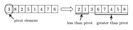
how does this help sort the array?
- the pivot element already winds up in its rightful position,
- partitioning has reduced the size of this problem: sorting the elements less than the pivot (which conveniently occupy their own subarray) and the elements greater than the pivot (also in their own subarray).
After recursively sorting the elements in each of these two subarrays, the algorithm is done
Therefore the algorithm is simply:
def quick_sort(A, n):
  if n <= 1:
    return A
  else:
    p = pivot(A, n)
    A_1, A_2 = partition(A, p)
    A_1_sorted = quick_sort(A_1, len(A_1))
    A_2_sorted = quick_sort(A_2, len(A_2))
    # if you can sort in place, you don't need this
  return A_1_sorted + [p] + A_2_sorted
Even though the quick runtime analysis above gives the same result as merge_sort, the quick_sort algorithm feels a bit different. This is because the order of operations is different. In merge_sort, the recursive calls are performed first, followed by the combine step, merge. In quick_sort, the recursive calls occur after partitioning, and their results don’t need to be merged at all!
But first of all, is this even correct? Here we prove it formally using induction, which is very suitable for recursive algorithms.
Proof of Correctness: We will prove by induction. Let $P(n)$ denote the statement “for any array $A$ of length $n$, quick_sort(A, n) returns a correctly sorted array”.
- Base case: $P(1)$ is trivially true, as the array is already sorted.
- Inductive hypothesis: assume $P(k)$ is true for all $k < n$, for any $n > 1$.
- Induction step. Now we need to imagine an input of $P(n)$. First, we note that the pivot element $p$ is already in the right sorted position. Then, we note that since
A_1andA_2are subarrays with size at most $n-1$, this means thatA_1_sortedandA_2_sortedare correctly sorted by the induction hypothesis. Therefore, the concatenation ofA_1_sorted,p, andA_2_sortedis also correctly sorted.
In-Place Partition
To sort the array in place using quick_sort, we just need a routine that can partition the array in place. This is a bit tricky, but it is possible to do this in a single scan over the array, while doing it in-place.
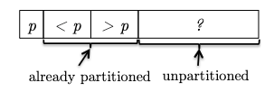
Key Idea: while scanning through the array, we can urge to keep the following invariant:
where to put the pivot element to the first position is just a swap in $O(1)$ during preprocessing. If we can check each new element in the unpartitioned part and swap it to the correct partition, then we can maintain this invariant = correctness!
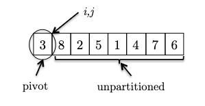
This is easiest to first go through an example. Consider an input:
where we consider the invariant formally to be:
Invariant: all elements between the pivot and $i$ are less than the pivot (the $< p$ partition), and all elements between $i$ and $j$ are greater than the pivot (the $> p$ partition). This means that:
- $i$ represent the boundary between the $< p$ and $> p$ partitions, and
- $j$ represent the boundary for yet unseen elements.
- We initialize $i,j$ to be right next to the pivot (first) element. As there is no element between $i$ and $j$ or between the pivot and $i$, the invariant is trivially satisfied.
- At each iteraction, we look at a new element and consider what to do to maintain the invariant:
 in this case $8$ is larger than the pivot and invariant is maintained.
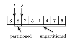
 - If the new element is smaller than the pivot. To maintain invraiant, we can swap it with the first element after $i$ and then increment $i$:
- We continue increment $j$ to see the new element. If it is bigger than the pivot, we can just continue as the invariant is maintained.
- One last, example, now we see another element smaller than the pivot, so we need to swap and increment $i$:
Hence the pseudocode is:
def partition_inplace(A):
  p = A[0]  # assuming pivot is the first element
  i = 1
  for j in range(1, len(A)):
    if A[j] < p:
      A[i], A[j] = A[j], A[i]
      i += 1
  A[0], A[i-1] = A[i-1], A[0]  # swap pivot to the correct position
  return A
Randomized QuickSort
Now, what about runtime? Again, the key step is how we choose the pivot element. Similar to DSelect, this will have a huge impact:
- if we choose min/max of the array, we get $\Omega(n^{2})$ runtime (technically also $O(n^{2})$, but just to emphasize the slowness).
- if we choose the median of the array, we get $T(n) = 2 T( n / 2) + O(n) = O(n \log n)$ where the $O(n)$ cost would be calling
DSelctto find the median.
While the median is the best choice, it is also the most expensive to compute. Therefore, we will use a randomized version of quick_sort that chooses a random pivot element. This is a very simple modification to the algorithm, and we will show that it has average case $O(n \log n)$!
Why on earth would you want to inject randomness into your algorithm? Aren’t algorithms just about the most deterministic thing you can think of? As it turns out, there are hundreds of computational problems for which randomized algorithms are faster, more effective, or easier to code than their deterministic counterparts.
To prove the average case runtime, let’s define some notations:
- sample space $\Omega$: the set of all possible outcomes of some random experiment
- random variable $X$: a (numerical) measurement of the outcome if a random process, so $X: \Omega \to \R$
- $P(\omega)$ is the probability of getting a particular outcome $\omega \in \Omega$.
In the case of quick_sort, we have:
- $\Omega$ being the set of all possible outcomes caused by some random (sequence of) choice of pivot element. (note that it is not defined on the length of the array)
- $X=RT$ that we care about is the runtime of this randomized
quick_sortgiven a sequence of pivot choices. I.e. given $w \in \Omega$, we get a deterministic runtime $RT(\omega)$.
So our goal is to find:
\[\mathbb{E}[RT] = \sum_{\omega \in \Omega} P(\omega) RT(\omega)\]But this $RT(\omega)$ is hard to compute. Taking a look at the algorithm, we notice that we can simplify this random variable to:
Lemma: For every input array $A$ of length $n \ge 2$ and every pivot sequence $\omega$:
\[RT(\omega) \le a \cdot C(\omega)\]for some constant $a > 0$, and $C$ denote the random variable equal to the total number of comparisons made between pairs of input elements performed by
quick_sortwith a given sequence of pivot choices.
See the book chapter 5.5 for more details, but on a high level: the main operation in quick_sort is the partition call, and that is where the comparisons are made.
But $C$ is still a difficult random variable. The trick is that we can decompose it further. Let $X_{ij}$ denote the total number of times the elements $z_i$ and $z_j$ get compared in quick_sort:
which literally represents the sum of all comparisons between pairs of elements in the array. Without loss of generality, let $z_i$, $z_j$ also be the $i$-th and $j$-th smallest elements in the array. Then, the question is how many times do we compare $z_i$ and $z_j$?
\[X_{ij}(\omega) = \{0,1\}\]because comparisons only happen during partition:
- if one of the elements is the pivot, then they can be compared at most once (and then they will be separated by the pivot and sent to different partitions)
- after they are separated, they will never be compared again.
Now the real trick is to use the linearity of expectation:
Linearity of Expectation: For any random variables $X_1, X_2, \dots, X_n$ and any constants $a_1, a_2, \dots, a_n$:
\[\mathbb{E}[a_1 X_1 + a_2 X_2 + \dots + a_n X_n] = a_1 \mathbb{E}[X_1] + a_2 \mathbb{E}[X_2] + \dots + a_n \mathbb{E}[X_n]\]In other words, the expectation of a sum of random variables is the sum of their expectations. Note that this is true even if the random variables are not independent.
Then we compute the expectation of $C$:
\[\begin{aligned} \mathbb{E}[C] &= \mathbb{E} \left[ \sum\limits_{i=1}^{n-1} \sum\limits_{j=i+1}^{n} X_{ij} \right] \\ &= \sum\limits_{i=1}^{n-1} \sum\limits_{j=i+1}^{n} \mathbb{E}[X_{ij}] \\ &= \sum\limits_{i=1}^{n-1} \sum\limits_{j=i+1}^{n} P(X_{ij} = 1) \\ &= \sum\limits_{i=1}^{n-1} \sum\limits_{j=i+1}^{n} P(\text{did compare $z_i$ and $z_j$ in QuickSort}) \end{aligned}\]Lemma If $z_i$ and $z_j$ denote the $i$-th and $j$-th smallest elements in the array, with $i < j$, then the probability that they are compared in
\[P(\text{did compare $z_i$ and $z_j$ in QuickSort}) = \frac{2}{j-i+1}\]quick_sortis:
Proof Sketch: Consider fixing $z_i$, $z_j$ with $i < j$, and let some pivot element $z_k$ be chosen during the first recursive call to quick_sort. What happens next?
- if $z_k$ is smaller than $z_i$ or bigger than $z_j$, then $z_i, z_{i+1}, …, z_{j}$ will be in the same partition, and will be sent to the next recursive call. They might be compared against in the future, we don’t know yet.
- if $z_k$ happens to be between $z_i$ and $z_j$, then $z_i$ and $z_j$ will be separated by the pivot, and are not and will never be compared again.
- if $z_k$ happens to be $z_i$ or $z_j$, then they will be compared once, and then separated by the pivot, and are not and will never be compared again.
Therefore, the first condition is just a “placeholder” that will eventually lead to the second or third conditions. So the probability of $z_i$ and $z_j$ being compared is equivalent to:
\[P(\text{$z_i$ or $z_j$ is chosen as the pivot before any other element in $z_{i+1}, ..., z_{j-1}$}) = \frac{2}{j-i+1}\]Finally we can compute the expectation of $C$ (hence the average runtime):
\[\begin{aligned} \mathbb{E}[\cdot C] &= \sum\limits_{i=1}^{n-1} \sum\limits_{j=i+1}^{n} P(\text{did compare $z_i$ and $z_j$ in QuickSort}) \\ &= \sum\limits_{i=1}^{n-1} \sum\limits_{j=i+1}^{n} \frac{2}{j-i+1} \\ &\le \sum\limits_{i=1}^{n-1} \left( 2 \sum\limits_{k=2}^{n} \frac{1}{k} \right) \\ &= 2n \sum\limits_{k=2}^{n} \frac{1}{k} \\ &\le 2n \log n = O(n \log n) \end{aligned}\]where
-
the third inequality comes from the fact that the largest sum we can get is when $i=1$:
\[\sum\limits_{j=i+1}^{n} \frac{1}{j-i+1} = \frac{1}{2} + \frac{1}{3} + ... + \left( \frac{1}{n} \right)\] -
the last inequality can be proven graphically:
where the sum covers the green highlighted rectangles, and the intergral covers the entire area under the blue curve.
Graphs: The Basics
Here we just go over some basics and notations, so that we are consistent for the rest of the course.
Representing Graphs: Let $G=(V,E)$ consist of vertices and edges. Let $n$ be the number of verticies and $m$ be the number of edges.
- note that if $G$ is undirected, then you will have $m \le { n \choose 2 }$
- note that if $G$ is directed, then you will have $m \le 2 { n \choose 2 } = n(n-1)$
Note that in either case, we have $m \le n^{2}$. Therefore in some proofs you will see, we might just swap $\log m$ with $\log n$ since:
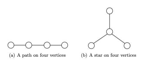
\[\log m \le \log n^{2} = 2 \log n \implies O(\log m) \le O(\log n)\]Tree a connected graph that has no cycles = have $n$ vertices and $n-1$ edges. For example:
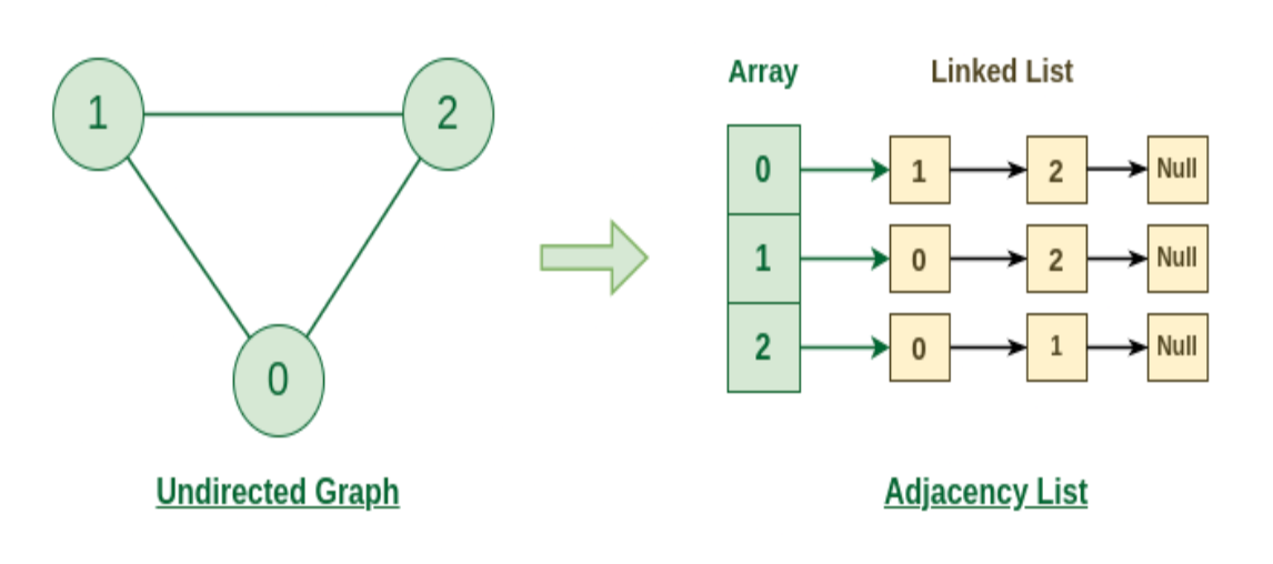
Ingredients for Adjacency List: the adjacency list representation of graphs is the dominant one we will use in this course. The main ingredients for representing such a list include:
- an array containing all the vertices
- an array containing all the edges
- for each edge, a pointer to each of its two endpoints
- for each vertex, a pointer to each of its incident edges so visually, something like this:
where essentially we have $V_0$ having neighbor [2,3,4], and $V_2$ having neighbor [1,8], etc. Or alternatively, you can think of it as:
But how much memory do we need to represent a adjaceny list? Well, we need:
- $O(n)$ space for the array of vertices
- $O(m)$ space for the array of edges
- $2m = O(m)$ space for the pointers to the edges’ endpoints. This is because each edge has two endpoints, hence $2m$.
- $2m = O(m)$ space for the pointers to the vertices’ incident edges. If you think about this, this is the same as the previous point, as the pointers to the edges’ endpoints are the same as (reversing) the pointers to the vertices’ incident edges.
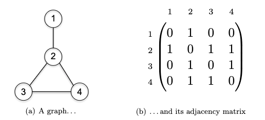
Therefore we need in total $O(n+m)$ space to represent a graph using adjaceny list. Note that this is more efficient than adjaceny matrix, which need $O(n^2)$ space:
Breadth-First Search and Depth-First Search
Both BFS and DFS would work whether if the graph is directed or undirected. On a high level, recall that
BFS Idea: start a vertex $s$ (layer 0), we want to explore all neighbors (layer 1), and repeat this process (reaching layer 2, layer 3, etc.) until we have explored all vertices.
So how do we implement it? The trick is to use a queue (FIFO) to keep track of the vertices still need to visit in the order of their discovery. The pseudocode is as follows:
def bfs(G, s):
  # let G be the adjaceny list representation of the graph
  # let s be the starting vertex
  explored[s] = True
  Q = Queue()
  Q.enqueue(s)  # initialize the queue with the starting vertex
  while Q is not empty:
    v = Q.dequeue()  # dequeue the first vertex in the queue
    for each edge (v, w) in G.adjacentEdges(v):  # explore all neighbors of v
      if not explored[w]:
        explored[w] = True
        Q.enqueue(w)  # enqueue the neighbor at the end
DFS Idea: when you reach a vertex, immediately start exploring its (not yet visited) neighbors and backtracking only when necessary (i.e. when you have no more neighbors to explore).
The most intuitive explanation is to talk about an example. Suppose we are given a graph, and the adjaceny list happened to give $s \to a$ before $s \to b$, then starting from $s$ we would go:
where the “frontier” marks the “borderline” between the explored and unexplored vertices. To make things interesting, let’s say the adjacency list had $c \to d$ before $c\to e$. This would then give us:
Now there is a problem: at vertex $e$ we have no unvisited neighbors. So DFS is forced to retreat to its previous vertex $d$: and now, it discovered one unexplored vertex $b$.
After this, DFS collapse quickly as each vertex has no unvisited neighbors, and DFS will eventually retreat all the way to $s$. If all neighbors of $s$ are visited, then DFS is done.
Therefore the pseudocode is as follows:
def dfs(G, s):
  # let G be the adjaceny list representation of the graph
  # let s be the starting vertex
  explored = {}  # mark all vertices as unexplored
  S = Stack()
  S.push(s)  # initialize the stack with the starting vertex
  while S is not empty:
    v = S.pop()  # pop the first vertex in the stack
    if not explored[v]:
      explored[v] = True
      for each edge (v, w) in G.adjacentEdges(v):  # explore all neighbors of v
        S.push(w)  # push the neighbor at the top
Why stack? If you think about the more “natural” recursive implementation, you will realize that essentially you are using a call stack. So the iterative implementation is just a “translation” of the recursive implementation.
Runtime of BFS/DFS: The running time for both algorithms is $O(n + m)$ being linear in the size of the graph. This is because both BFS/DFS will:
- examine each vertex at most once
- examine each edge at most twice (once for each endpoint) therefore the total number of operations is $O(n + 2m) = O(n + m)$.
Generic Search
Is BFS and DFS correct? How do we prove that its runtime is $O(n+m)$? The answer is to realize that they both fall into the pattern of a generic search algorithm:
def generic_search(G, s):
  # let G=(V, E) be the adjaceny list representation of the graph
  # let s be the starting vertex
  explored = {s} # mark s as explored, others as unexplored
  while there is an edge (v,w) in E with v explored and w unexplored:
    choose some such edge (v,w)
    explored.add(w)
To see why this could contain both BFS and DFS, consider the following example graph:
- initially only our home base $s$ is marked as explored.
- In the fist iteration of the while loop, two edges meet the loop condition: $( s, u )$ and $( s, v )$. The GenericSearch algorithm chooses one of these edges — $(s, u)$, say — and marks $u$ as explored.
- In the second iteration of the loop, there are again two choices: $( s, v )$ and $( u, w )$. The algorithm might choose $( u, w )$ being DFS-like or $( s, v )$ being BFS-like.
Correctness of Generic Graph Search: At the conclusion of the
generic_search, a vertex is $v \in V$ is explored if and only if there is a path from $s$ to $v$ in $G$.
- this also means that every vertex $v$ is explored
- for BFS/DFS, it is then easy to see that each vertex is also explored only once (if reachable)
Proof: This is IFF proof, so we need to argue from both directions.
\[\text{$v$ is explored in generic\_search} \implies \text{there is a path from $s$ to $v$ in $G$}\]this is trivially true, as the only way we can discover $v$ is by following paths from $s$.
\[\text{there is a path from $s$ to $v$ in $G$} \implies \text{$v$ is explored in generic\_search}\]This basically says that the generic_search algorithm didn’t miss any vertex. We can prove this by contradiction: let there be a path from $s\leadsto v$, but `generic_search` halted and missed it. The intuition is that this cannot be, because we checked every edge given a vertex. More formally, let $S \subseteq V$ be the set of vertices just now marked as explored by the algorithm. Then vertex $s \in S$ and, by assumption, $v$ does not. But since there is a path from $s \leadsto v$, then there must exist a path from a vertex in $S$ going to one outside $S$ (reaching $v$). Then, our algorithm would have picked this during the while loop, and the algorithm would have at least explored one more vertex instead of halting, and would have eventually reached $v$. This is a contradiction, as we assumed that the algorithm halted and missed $v$.
Computing connected Components
This is one typical application of BFS/DFS. Let’s use BFS here.
Recall that
Connected Component is a maximal set of vertices $S \subseteq V$ such that for every pair of vertices $u,v \in S$, there is a path from $u$ to $v$ in $G$. Visually:
Consider $G=(V,E)$ being an undirected graph, and consider the task being to identify all connected components of $G$ (e.g. assign each vertex v a label cc(v) indicating which connected component it belongs to).
The idea is simple: we can use an outer loop to make a single pass over the vertices, and invoke BFS as a subroutine whenever we encounter an unexplored vertex. The pseudocode is as follows:
def ucc(G):
  # let G be the adjaceny list representation of the graph
  cc = {}  # mark all vertices as unexplored
  num_cc = 0  # number of connected components
  for each vertex v in G.vertices:
    if not explored[v]:
      cc[v] = v  # label the connected component
      num_cc += 1  # increment the number of connected components

      ### BFS subroutine
      Q = Queue()
      Q.enqueue(v)  # initialize the queue with the starting vertex
      while Q is not empty:
        w = Q.dequeue()  # dequeue the first vertex in the queue
        for each edge (w, x) in G.adjacentEdges(w):  # explore all neighbors of w
          if not explored[x]:
            explored[x] = True
            cc[x] = v  # assign the same connected component to x
            Q.enqueue(x)  # enqueue the neighbor at the end
  return cc
What’s the runtime? Although this looks like looping over $O(m+n)$ which is the cost of BFS, in fact we note that BFS/DFS$(G,s)$ is technically linear in the size of the connected component of $s$. Therefore the runtime is:
\[\underbrace{O(n)}_{\text{looping over every vertex}} + O\left( \sum \text{connected component's size} \right) = O(n) + O(n + m) = O(n + m)\]Topological Sort
Here is another classic application of DFS. Imagine that you have a bunch of tasks to complete, and there are precedence constraints, meaning that you cannot start some of the tasks until you have completed others. ne application of topological orderings is to sequencing tasks so that all precedence constraints are respected. More formally
Topological Orderings: let $G=(V,E)$ be a directed graph. A topological ordering of $G$ is an assignment $f(v)$ of every vertex $v \in V$ to a different number such that:
\[\text{for every }v\to w \text{ edge}, f(v) < f(w)\]i.e. all of $G$’s directed edges should travel forward, with the arrow heading pointing to a vertex with a higher number.
Visually, consider the following example:
and there are two ways to topologically sort this graph:
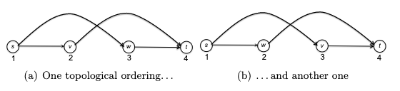
You can visualize a topological ordering by plotting the vertices in order of their f-values. In a topological ordering, all edges of the graph are directed from left to right.
Note that this means, it is impossible to topologically order the vertices of a graph that contains a directed cycle. Therefore, in general a topological order exists only for a directed graph without any directed cycles - a directed acyclic graph (DAG).
In fact
Theorem 8.6: Every DAG has a topological ordering.
To show this, first realize that
Theorem 8.7: Every DAG has a source.
- proof: if you keep following incoming edges backward out of an arbitrary vertex of a directed acyclic graph, you’re bound to eventually reach a source vertex. Otherwise, there would be a directed cycle.
- i.e.: if you DFS and is stuck in a DFS, then there is a cycle in your graph.``
where:
- A source vertex of a directed graph is a vertex with no incoming edges.
- Analogously, a sink vertex is one with no outgoing edges.
Then, we can prove Theorem 8.6 very easily. Let $G$ be a directed acyclic graph with $n$ vertices. The task is to assign $f$-values to vertices in an increasing order:
- the source vertex will be assigned 1
- obtain $G’$ by removing the source vertex and all its outgoing edges. Note that this cannot produce a directed cycle, as deleting stuff can’t create new cycles
- repeat from step 1 on $G’$
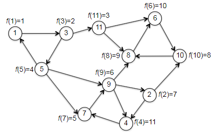
So how to do compute a topological sorting, i.e. output a topological ordering of the vertices of a DAG $G$?
- the proof above naturally leads to an algorithm: a loop ($O(n)$) over each vertex where we find the source ($O(n)$), and then deleting it to repeat. This gives us $O(n^2)$.
- next up: a slicker solution via DFS resulting in $O(n+m)$.
First we show the algorithm, the high level idea is simple: we use DFS to dive to the sink and assign the lowest ordering to it, but also assign things during backtracking!. We then mark it as explored (i.e. as if we removed the vertex from G) and repeat.
curLabel = |V|  # tracks the ordering
f = {}  # topological ordering

def topo_sort(G):
  # let G = (V, E) be the adjaceny list representation of the graph
  # let s be the starting vertex
  explored = {}  # mark all vertices as unexplored
  for each vertex v in G.vertices:
    if not explored[v]:
      dfs_topo(G, v, explored)
  return

def dfs_topo(G, s, explored):
  global curLabel, f

  explored[s] = True
  for each edge (s, w) in s outgoing adjaceny list:
    if not explored[w]:
      dfs_topo(G, w, explored)
  f[s] = curLabel  # assign the ordering
  curLabel -= 1  # decrement the ordering
  return
note that topo_sort doesn’t need to us to start at a particular vertex. We can start at any vertex, and the algorithm will still work. (Basically the algorithm dives as deep as possible, and assign that deepest vertex (regardless which starting vertex you choose) with $f(\cdot) = \vert V\vert$.)
Correctness: first of all, it is obvious to see that:
- every vertex $v$ is assigned a unique number $f(v)$, as each is called by
dfs_topoonly once. - to argue why the returned
fmust be a topological order, we need to show for any arbitrary edge $(v,w)$ such that $v\to w$, we have $f(v) < f(w)$.
Proof if there is an edge $(v,w)$, then there are two cases in running topo_sort:
- if $v$ is explored before $w$, i.e. we
dfs_topois invoked with vertex $v$ before $w$ is explored. Then as $v \to w$ is reachable, we will get a call stack of [dfs_topo(v)->dfs_topo(w)]. Since the nature of recursive call will meandfs_topo(w)will terminate first, it will be assigned a higher ordering thandfs_topo(v). Therefore $f(v) < f(w)$. - if $w$ is explored before $v$, then it means there cannot be a path from $w$ back to $v$ (because we already have $v \to w$ and we know the graph is a DAG). Therefore, the call
dfs_topo(w)will terminate without callingdfs_topo(v). Then, astopo_sortwill eventually calldfs_topo(v)later, it means $v$ will get a lower ordering. Hence $f(v) < f(w)$.
Runtime: runs in linear time $O(n+m)$, as it is just DFS with a little extra bookkeeping:
- it explores each edge only once (from its tail), only performs a constant amount of work per edge/vertex
- therefore, the runtime is $O(n+m)$
Computing Strongly Connected Components
In short, while it didn’t matter much for undirected graph, for directed graph having a connected component makes things more complicated. First, recall that a connected component for undirected graph is defined as maximal regions within which you can get from anywhere to anywhere else in the region. For directed graph, consider
Following the logic, the answer should be zero.
Strongly Connected Component (SCC) a maximal set of vertices $S \subseteq V$ such that there is a directed path from any vertex in $S$ to any other vertex in $S$.
For example
First of all, why would ucc not work? Consider evoking BFS on the following vertices

first, notice all the edges are organized to go mainly from left to right. In the case on the left, we would get a wrong result: BFS will discover every vertex and mark them as the same connected component. In the case on the right, we would get a correct result. This indicates that graph search can uncover strongly connected components, provided you start from the right place. But how? The key observation is that we want to first start from a sink SCC, i.e. the SCC with no outgoing edges to other SCCs. Then, we can go in a reverse topological order, plucking off sink SCCs one by one.
Key Lemma: the SCC Meta-Graph is directed acyclic. Visually this is simple to see:
and the argument is also simple. If two meta SCC are not acyclic, then you would have collapsed them into one, i.e., the two meta SCC were not maximal at the first place.
- this lemma is actually very important. This means that all we need to do is to find one vertex in a sink SCC, run BFS/DFS to label all vertices it can reach (and mark them as explored), and repeat
- the above works because for a directed acyclic graph + using a sink SCC, you cannot get out of that sink SCC.
On a high level, the arguments above in the lemma is pretty much what we will do, except you might be a bit confused by the graph reversing step
# sktech of Kosaraju’s algorithm
def kosaraju_idea(G):
  G_rev = reverse(G)  # reverse the graph, i.e. reverse all edges
  dfs_loop(G_rev), let f[v] = "finishing time" of DFS on a vertex v
  dfs_loop(G), using f to process vertices in decreasing order  # i.e. start from the sink vertex
  return vertices with their labels
while yes, the second relates to some kind of topological order, and third step relates to us wanting to get a reverse topological order before diving DFS to label the vertices. But there are a few caveat:
- second step did something on a reversed graph. Why?
- we thought about the
topo_sortalgorithm only in DAGs, and here we have a general directed graph. - the second and third is not equivalent to
topo_sortof a normalGand then start from the sink vertex.
So what’s going on? First we show the full algorithm, and then we will illustrate how it works, and why it is correct.
global numSCC: int

def Kosaraju(G):
  # let G = (V, E) be the adjaceny list representation of the graph
  G_rev = reverse(G)  # reverse the graph, i.e. reverse all edges
  mark all vertices in G_rev as unexplored

  # first pass of DFS
  # computes f(v), the magical ordering
  TopoSort(G_rev)

  # second pass of DFS
  # finds SCCs in reverse topological order
  mark all vertices in G as unexplored
  global numSCC = 0  # number of SCCs, global variable
  for each v in V, in increasing order of f(v):
    if not explored[v]:
      numSCC += 1
      # assign scc-values for all vertices in the SCC
      dfs_scc(G, v)

def dfs_scc(G, s):
  global numSCC
  explored[s] = True
  scc[s] = numSCC
  for each edge (s, w) in s outgoing adjaceny list:
    if not explored[w]:
      dfs_scc(G, w)
  return
So, it turns out all the concern above will be addressed after thinking about this.
Why reverse graph + topological sort?
What we want, in the end, is to find a vertex in a sink SCC of $G$. The hope with topo_sort is that, we recall, the vertex in the last position ($f(v)=\vert V\vert$) must be a sink vertex (hence inside sink SCC) of $G$. However, it was for DAGs. So are we lucky enough that this would hold for a general graph? The answer is sadly no. If we consider the following example where we started at vertex 1 (recall that topo_sort starts at random vertex):
| correct source but wrong sink | correct source and correct sink |
|---|---|
 |
 |
where basically the left is made by trying to start at vertex 1 and wind up ending at vertex 4 during the first iteration, while the right is made by starting at vertex 1 and ends at vertex 8 during the first iteration of topo_sort. Although we couldn’t consistently find a vertex in a sink, it turns out we can consistently find a vertex in the source SCC. But in fact, the statement is even stronger: tThe topological order of the SCCs will also be a topological ordering of the meta-graph, if we label each SCC with the smallest $f$ of one of its vertices, i.e. formally
Theorem 8.10: Topological Ordering of the SCCs. Let $G$ be a directed graph, with vertices ordered arbitrarily, and for each vertex $v \in V$ let $f(v)$ be the position of $v$ computed by
\[\min_{x \in S_1} f(x) < \min_{y \in S_2} f(y)\]topo_sort. Let $S_1, S_2$ denote two SCCs of $G$, and suppose $G$ has an edge $(v,w)$ with $v \in S_1$ and $w \in S_2$, then:i.e. even if
topo_sortis incorrect in this case globally for every vertex, it is still correct locally for the SCCs!.
the proof is similar to the correctness of topo_sort. If we consider the following illustration:
then there are two cases that can happen during topo_sort labeling all the vertices:
topo_sortexplored and initialized a DFS from a vertex $s \in S_1$ before any vertex in $S_2$. But because we know vertices in a SCC can reach each other, then $s \leadsto v$, and since $v \to w$, then we can reach from $s$ to any vertex in $S_2$. Therefore, becausetopo_sortis a DFS/recursive call, the calldfs_topo(s)will not terminate until all the vertices in $S_2$ terminates. Therefore, $f(v)$ must also be smaller than $f(w)$.topo_sortexplored and initialized a DFS from a vertex $s \in S_2$ before any vertex in $S_1$. Then, because the meta-graph is directed acyclic, we are stuck in $S_2$, and $S_1$ will be unscathed. Since the counter for $f$ is a global variable, this means we will get a smaller $f$ for $S_1$ than $S_2$.
The end result? We are sure that the first vertex resides in a source SCC if we do topo_sort. So to find a vertex in a sink SCC, all we need is to reverse the graph first.
Finally, an example before going to the correctness and runtime discussion. We want to check that the magical reverse graph + topo_sort will indeed help us get vertices in a sink SCC, and so that the second pass of depth-first search discovers the SCCs in reverse topological order.
| $G_{rev}$ and compute $f(v)$ | $G$ with computed $f(v)$ |
|---|---|
 |
 |
Then, given the progress above (by reversing the graph and calling topo_sort), we continue to the second pass to DFS, which checks through vertices in increasing order:
- first call to DFS-SCC is initiated at the vertex 1 with smallest $f$. (the vertex in a sink SCC!)
- then it will label all vertices $1,3,5$, and mark as done.
- the second smallest and third is with vertex 3, which is visited already.
- the third smallest is vertex 11, which is also (a vertex in) the second sink SCC.
- continues
Correctness and Runtime of Kosaraju’s Algorithm
The argument will be short as the proofs are mostly covered in the previous section.
Correctness: each time we initiates a new call to dsf_scc, the algorithm discovers exactly one new SCC - the sink SCC relative to the not-yet-explored part of the graph.
Runtime: each of the two passes of DFS does a constant number of operations per vertex or edge. Therefore, the runtime is $O(n+m)$.
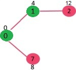
Dijkstra’s Shortest Path Algorithm
We’ve arrived at another one of computer science’s greatest hits: Dijkstra’s shortest-path algorithm.
Assumptions with Dijkstra’s Algorithm: this algorithm works in any directed graph with nonnegative edge length.
- can we extend it to undirected graph? (Yes, by changing the ‘frontier’ condition)
- can we extend it to negative edge length? (No, but Bellman-Ford can)
Problem definition: consider a directed graph $G=(V,E)$, a starting vertex $s \in V$, and a nonnegative length $l_e$ for each edge $e \in E$. The goal is to compute the length of a shortest path $D(v)$ from $s$ to every other vertex $v$ in $G$.
Why can’t we use BFS? Remember that breadth-first search computes the minimum number of edges in a path from the starting vertex to every other vertex (i.e. we continue layer by layer). This is the special case of the single-source shortest path problem in which every edge has length 1.
- but then can’t we just think of an edge with a longer length $l>1$ as a path of edges that each have length 1?
- Yes, in principle, you can solve the single-source shortest path problem by expanding + using BFS
- However, the problem with this is that it blows up the size of the graph
Dijkstra’s Algorithm
The idea of Dijkstra’s algorithm is to use a greedy approach: at each step, we will grow the frontier by one vertex. Overall it looks similar to BFS/DFS by iterating over the new vertices, but the clever part is how we choose which vertex to process next/is done.
Consider some example graph, where each edge $e$ has a length of $l_e$:
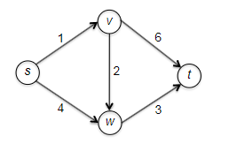
Consider the pseudo-code
def dijkstra(G, s):
  # let G = (V, E) be the adjaceny list representation of the graph
  # let s be the starting vertex
  X = {s}  # list of vertices processed so far
  dist[s] = 0 # tracks the cost of shortest path distance
  path[s] = []  # tracks the shortest path, empty for s

  while there is an edge (v,w) with v in X and w not in X:  # check edges that crossed the "frontier"
    (v*, w*) = edge minimizing dist[v] + l_vw
    X[w*] = True  # grow exactly one vertex
    dist[w*] = dist[v*] + l_vw
    path[w*] = path[v*] + [w*]

  return dist, path
Visually, this works like:
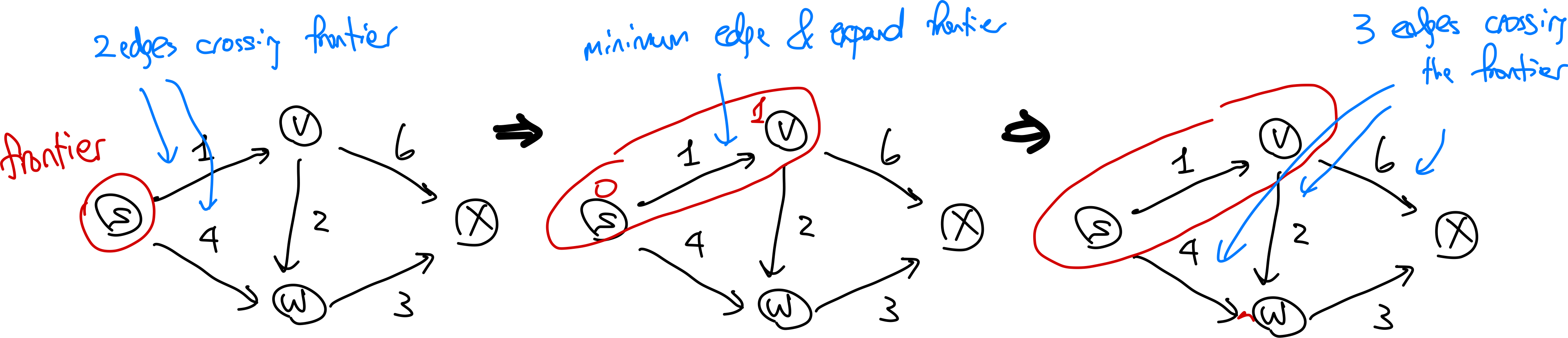
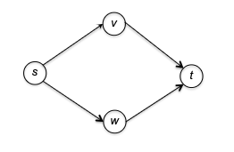
Is this algorithm correct? If you think about it, this is what Dijkstra’s algorithm is trying to say. Consider an edge $(v,w)$ with $v \in X$ and $w \notin X$. Then the shortes path from $s$ to $w$ consists of the shortest path from $s$ to $v$ (or $s \leadsto v$) with edge $(v,w)$ tacked at the end. So is this correct?
Correctness of Dijkstra’s Algorithm
Essentially Dijkstra’s algorithm iterates over the entire $V$ space, so we can consider induction on the number of vertices $n$.
Proof: Let $P(n)$ denote that “the Dijkstra algorithm correctly computes the shortest-path distance of the $n$th vertex added to the processed set $X$”. We will prove this by induction on $n$:
- Base case: $P(1)$ is trivially true, as the starting vertex $s$ is the first vertex in $X$ and the shortest path distance from $s$ to $s$ is indeed $0$.
- Inductive hypothesis: Let $P(k)$ be true for all $k=1,2,3…, n-1$. This means that we have $d(v)=\mathrm{shortest}(s,v)$ correctly computed for the first $n-1$ vertices added by Dijkstra to $X$.
-
Inductive step: now we need to show $P(n)$. Let $w^{}$ be the $n$th vertex being added, and let Dijkstra to have selected the $(v^*, w^*)$ edge for that to happen (i.e. $v^{}\to w^{*}$ is the shortest edge at the frontier). We need to show that:
\[d(v^*) + l_{v^{*}w^{*}} = \mathrm{shortest}(s, w^*)\]We can show this by:
- showing $d(v^) + l_{v^{}w^{}} \ge \mathrm{shortest}(s, w^)$, that the shortest path can only be less than or equal to the path from $s$ to $v^$ plus the edge $(v^, w^*)$. This is trivially true by definition of the shortest path.
-
showing $d(v^) + l_{v^{}w^{}} \le \mathrm{shortest}(s, w^)$, namely every competitor path $s \leadsto w^{}$ must be at least $d(v^) + l_{v^{}w^{}}$. To show this, consider a “crazily short” path:
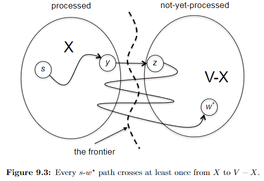
where because we know that path has to start at $s$ and ends at $w^{*}$ which is outside $X$, then it must have crossed the frontier at some point. Let’s denote the first edge from that path crossing the frontier be $(y,z)$, such that $y\in X, z \notin X$. So in essence we can considering any competitor path $P’$ taking the form:
\[P' = \underbrace{s \leadsto y}_{\text{inside X}} \to z \leadsto w^{*}\]we note that this path must has at least:
\[len(P') \ge \text{shortest}(s,y) + l_{yz} + 0 = d(y) + l_{yz}\]where we used $+0$ because we assumed no edges can be negative, and that $d(y) = \text{shortest}(s,y)$ from the inductive hypothesis. But we notice that this $d(y) + l_{yz}$ exactly represents an edge that just crossed the frontier. This means that according to Dijkstra’s algorithm that since we picked $(v^{}, w^{})$ edge:
\[d(y) + l_{yz} \ge d(v^{*}) + l_{v^{*}w^{*}}\]Therefore every competitor path $P’$ must be at least $d(v^) + l_{v^{}w^{*}}$, and we are done. (Intuitively, this is saying that *any path $P'$* going outside of $X$ will need to use the shortest path inside $X$ + something outside $X$, and while Dijkstra is minimizing exactly this, it works.)
Q: What if we are dealing with a directed graph that has negative edges, but let’s say, no negative cycles?
The main insight here is that the algorithm only looks at all directly connected edges and it takes the smallest of these edge. The algorithm does not look ahead.
Therefore, you can consider the following example (from stackoverflow)

where Dijkstra would return the shortest path from $A\leadsto D$ being at a cost of 2, but in reality it is $-4900$.
Q: is there a case where Dijkstra algorithm is still correct despite there are negative edges?
Yes. Consider a directed graph $G$ and a starting vertex $s$ with the following properties: no edges enter the starting vertex $s$; edges that leaves have arbitrary (possibly negative) lengths; and all other edge lengths are nonnegative. Dijkstra’s algorithm correctly solve the single-source shortest path problem. You can see this in two ways:
- notice that adding the same positive constant $M$ to each of s’s outgoing edges preserves all shortest paths, as the lengths of all the $s \leadsto v$ path goes up by precisely $M$
- go back to the formal correctness proof of Dijkstra, and realize that the induction step would still work.
Hash Tables and Bloom Filters
The goal of a hash table is to facilitate super-fast searches, which are also called lookups in this context. Compared to other data structures we will discuss later (e.g. heaps and search trees), hash tables do not maintain any ordering information.
A hash table keep track of an evolving set of objects with keys while supporting fast lookups (by key).
e.g. if you company manages an e-commerce site, you might use one hash table to keep track of employees (perhaps using names as keys).
Hash Table Operations: a hash table needs to support the following operations:
- insert: given a new object $x$, add it to the hash table
- lookup: given a key $k$, return a pointer to an object in the hash table with key $k$ (or null if no such object exists)
- delete: given a key $k$, remove the object with key $k$ from the hash table, if it exists
(for programming purposes you can just imagine the key a numerical representation of the object (e.g. memory address of the object), and a hash function $h$ operates on the key $h(k)$)
and to really be a hash table:
| Operation | Typical/Average Runtime |
|---|---|
| Lookup | O(1)* |
| Insert | O(1) |
| Delete | O(1)* |
where:
- the asterisk (*) indicates that the running time bound holds if and only if the hash table is implemented properly (with a good hash function and an appropriate table size) and the data is non-pathological (see later).
- insert is technically always $O(1)$, not average runtime.
Since this is really for fast lookups, example applications of hash tables include:
- 2-SUM problem: given a target $t$ and a list of integers $A$, find two distinct integers $x,y \in A$ such that $x+y=t$.
- realize that given a $x$, there is only one possible $y$ that can achieve this = just look up $t-y$!
- deduplication: given a list of $n$ items, remove all duplicates in $O(n)$ time
- first check if the hash table already has the key, if not, insert the k and store the object
Implementation: Separate Chaining
So how do we get a (near) constant lookup time? Here we discuss a very common implementation of hash tables, which is called separate chaining (and the other popular one is called open addressing). We will first discuss separate chaining.
Visually, this is very easy to understand:
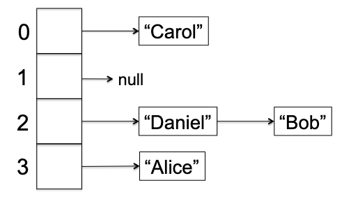
so that:>
Separate Chaining: Let there be an array $A$ of $n$ buckets, and for each bucket you have a linked list so that given a key $k$, lookup/insert/delete essentially all operate on the linked list $A[h(k)]$.
- note that this means your hash function needs to do $h: U \to {0,1,2,…,n-1}$ where $U$ is all possible objects/keys, which can be achieved by simply doing modulo n.
But now we get some problems:
- insert is surely constant time
-
but lookup and delete technically need:
\[\text{Runtime(lookup/delete)} = O(\text{length of linked list})\]
So our goal is to keep small linked list for each bucket. First of all, in what cases can we get bad performance?
- Size of $n$ is too small, so that we have too many collisions.
- This is easy to fix: just increase the size of $n$. But then you also need to rehash everything.
- Using a bad hash function (e.g. $h(k) = 0$ a constant function).
- So then what is a good hash function? One that Mimics a random function by spreading non-pathological datasets (see below) roughly evenly across the positions of the hash table
- The data is pathological, i.e. it is always possible to adversarially come up with some kind of data such that they all hash to the same bucket. i.e. for every hash function $h: U \to {0,1,2,…,n-1}$, there exists a set $S$ of keys such that $h(k_1) = h(k_2)$ for every $k_{1}, k_{2} \in S$.
- this is unfixable. The best we can do is to assume that the data is not pathological.
Takeaway: while 1 and 2 are somewhat avoidable, condition 3 means that hash tables cannot guarantee $O(1)$ for lookup or delete.
However, we can guarantee $O(1)$ is average runtime under some conditions (actually all the three will need to be addressed)
Claim: let there be a dataset $S$. If our hash table has a reasonably big size $\vert S\vert =O(n)$ (condition 1), and $h(x)$ is like a random function (condition 2), and $S$ is not pathological (condition 3), then the average runtime of lookup and delete is $O(1)$.
Proof: since we are discussing average time, the procedure will be similar to quick sort analysis. We begin by figuring out the random variable we want to analyze, then decompose it to simpler random variables, and finally use linear expectation to get the result.
Suppose you have inserted all $s \in S$ into the hash table. Consider a lookup for a new random object $x$ with key $k$, which might or might not be in $S$. Then the runtime is:
\[\mathrm{Runtime} = O(\text{list length of }A[h(k)]) = O(l)\]where $l$ is the random variable as it could be long or short. But notice that
\[O(l) = O(\# \text{of collisions $x$ is making})\]This means that:
\[\begin{align*} l \le 1 + \sum\limits_{y \in S, y \neq x} z_{y} \end{align*}\]where $z_y$ is (again) an indicator random variable indicating if there is a collision, and the one is there if there is a $y=x$ (i.e. essentially $x$ was an object $S$).
\[z_{y} = \begin{cases} 1, & \text{if $h(x)=h(y)$ } \\ 0, & \text{otherwise} \end{cases}, \quad \forall y \in S\]Now decomposition is complete, we realize that:
\[\begin{align*} \mathbb{E}[l] &\le \mathbb{E}\left[1 + \sum\limits_{y \in S, y \neq x} z_{y}\right] \\ &= 1 + \sum\limits_{y \in S, y \neq x} \mathbb{E}[z_{y}] \\ &= 1 + \sum\limits_{y \in S, y \neq x} \Pr[h(x)=h(y)] \end{align*}\]But we realize that if $h$ is a perfectly random hash function, then $\Pr[h(x)=h(y)]$ given an $x$ is like throwing the $y$ dart randomly at the $n$ buckets, and hoping that it lands on the same bucket as $x$. Therefore, the probability is $1/n$. Hence we get:
\[\begin{align*} \mathbb{E}[l] &\le 1 + \sum\limits_{y \in S, y \neq x} \Pr[h(x)=h(y)] \\ &= 1 + \sum\limits_{y \in S, y \neq x} \frac{1}{n} \\ &= 1 + \frac{|S|-1}{n} \\ &= O(1) \end{align*}\]where the last equality is because we had said $\vert S\vert =O(n)$, i.e. our hash table is reasonably big.
Implementation: Open Addressing
Why did we have a linked list version before (i.e. separate chaining)? In the end it was to resolve collision, but letting them live in the same bucket. Note that such collision is inevitable, as we have fixed size of data structure but your dataset $S$ is huge.
The idea of open addressing is, instead of letting the collision live in the same bucket, we will try to find another bucket for the colliding object, assuming $n \ge \vert S\vert$. In this implementation, each bucket stores only 0 or 1 object.
Open Addressing: given an object $x$ with key $k$ and its position to insert $h(k)$. We will use some probe sequence (i.e. a sequence of buckets to check) if $h(k)$ is occupied.
- so for insert, we continue this sequence until the first empty bucket, and insert the object there
- for lookup, we continue this sequence until we find the bucket storing $x$, or an empty bucket (return not found)
- we will not support delete.
So the trick is this “probe sequence”. One simple sequence would be a linear probing: $h(k), h(k)+1, …, \text{wrap around}, h(k)-1$.
We skip other details here, but discuss its performance compared to separate chaining.
- with chaining, the lookup time is affected by linked list length; with open addressing, its the number of probes required to either hit an empty slot or find the object.
- in both implementations, when the hash table gets increasingly full, performance degrades.
- however, with an appropriate hash table size and hash function, open addressing achieves the same running time bound as chaining.
Bloom Filters
Bloom filters have became a very popular data structure since its usage in internet routers. It has a very similar idea to hash tables, but:
- it is more space efficient
- it can only return
true/falsefor lookup (i.e. if the object is in the set or not) - it can return false negatives (i.e. even if the object is not in the set, it might return
true) - it guarantees constant-time operations for every dataset.
Blook Filter Supported Operations: a bloom filter supports the following operations:
- lookup: given a key $k$, return
trueif $k$ is in the bloom filter, andfalseif $k$ is not in the bloom filter- insert: add a new key $k$ to the bloom filter (since we are only returning
true/falsefor lookup, we don’t need to store the key/object itself)
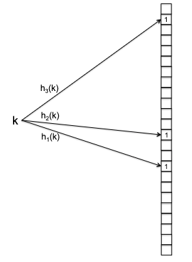
The idea of Bloom filter is simple. Consider an array of $n$ bits all initially zero. Then the data structure uses $m$ hash functions $h_1, h_{2}, …, h_m$ each mapping $h_{i} : U \to { 0,1,2, … , n-1 }$.
- you can create $m$ hash functions *using one real hash function $h_{}$*, by doing $h_{1}(k) = m \cdot h_(k), h_{2} = m \cdot h_*(k) + 1$, etc.
- typically $m$ is quite small, like $m=5$.
Then the operations is simply:
def insertion(k):
  # flip all A[h_i(k)] = 1
  for i in range(m):
    A[h_i(k)] = 1

def lookup(k):
  # check if all A[h_i(k)] == 1
  for i in range(m):
    if A[h_i(k)] == 0:
      return False
  return True
Visually:
hence it is obvious that:
- you cannot get false negative: if an object is in the set, then its bits must have been flipped to 1 (as we are not supporting deletion).
- you can get false positive: if an object is not in the set, then its bits might have been flipped to 1 by other objects.
Now, error analysis: is this really worth it? How much error will this give? The goal is to get a $n$ not too large but still have a small false positive rate.
Suppose that we have inserted all elements $x \in S$ into the bloom filter. Consider a lookup for a new random object $x$ with key $k$, which is a false positive. For this to happen, we need:
\[\Pr[\text{false positive}] = \Pr[\text{all $m$ bits are flipped for $x$}] = \Pr[ \text{one bit is flipped} ]^{m}\]What’s the probability that one bit is flipped?
\[\Pr[ \text{one bit is flipped} ] = 1 - \Pr[ \text{all data missed that bit} ] = 1 - {\underbrace{\left( 1 - \frac{1}{n}\right)}_{\text{one hash function missed}}}^{m |S|}\]where its raised to the power of $m \vert S\vert$ since there are $\vert S\vert$ objects we inserted, and for each object we had $m$ “dart shots” (recall that we assume $h$ is a perfectly random function). This form approximates that of an exponential function:
\[\Pr[ \text{one bit is flipped} ] = 1 - {\left( 1 - \frac{1}{n}\right)}^{m |S|} \approx 1 - e^{- m|S| / {n}}\]finally:
\[\Pr[\text{false positive}] \approx \left( 1 - e^{- m|S| / {n}} \right)^{m}\]Notice that this is a function of $n,m, \vert S\vert$. Therefore, depending on the application, we can optimize for the error rate (using calculus), if we fix $n / \vert S\vert$ representing the number of bits per object:
\[m^{*} = \frac{n}{|S|} \ln 2\]this means that if we are having an array for about 8 bits per object, then we should use $m=5 \sim 6$ hash functions which gives an error rate of about 2%.
Introduction to Greedy Algorithms
This is another class of algorithm, where compared to the divide and conquer algorithm:
| Divide and Conquer | Greedy Algorithms |
|---|---|
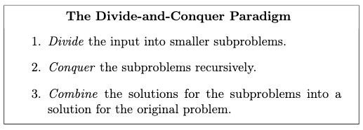 |
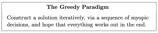 |
| relatively easy to prove correct (e.g. induction) | usually hard correctness proof |
| harder to analyze runtime | usually straightforward sorting + single pass |
While it is myoptic and simple to implement, it is often hard to come up with a correct greedy algorithm (e.g. Dijkstra was one), and for many problems there might not exist a correct greedy algorithm. More specifically, you shall see that correctness proofs for greedy algorithms are more art than science, though there will be a useful trick, called the exchange argument, which we will show next.
Scheduling Problem
Consider the scheduling task in OS, where given some set of jobs $J$ with each job $j$ having known length $l_j$ (i.e. how long it takes to complete), and a weight $w_j$ (e.g. priority). We want to have a scheduling algorithm that can find the “best” sequence of jobs to complete $\sigma$. What is a “best” schedule?
-
first of all, how many posisble schedules are there? $n!$.
- completion time $C_j(\sigma)$ of a job $j$ is the sum of lengths of the jobs preceding $j$ in $\sigma$, plus the length of $j$ itself. i.e. time elapsed when $j$ is completed.
- e.g. consider three jobs with length $l_1=1, l_{2}=2, l_3=3$, weight $w_1=3, w_2=2, w_{3} = 1$. Suppose we scheduled them to be in the order of $j_1, j_2, j_3$. Then this means the completion time is $C_{1} = 1, C_{2} = 3, C_{3} = 6$. Visually
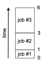
-
sum of weighted completion times. This is our objective function:
\[\min_\sigma \sum\limits_{j =1}^{n} w_j C_j(\sigma)\]i.e. we want shorter/more important jobs to be completed earlier.
Scheduling Task: given a set of $n$ jobs with positive lengths $l_j$ and positive weights $w_j$, find a schedule $\sigma$ that minimizes the sum of weighted completion times.
To solve this problem, let us first posit that there actually is a correct greedy algorithm for the problem. Then, we need to consider some intuitions by thinking about some "special cases".
Intuition:
- if all job lengths are equal, then we should schedule jobs with a higher weight first.
- if all job weights are equal, then we should schedule shorter jobs first. (Why? Realize that in general, the job scheduled first contributes to the completion times of all the jobs, as all jobs must wait for the first one to finish.)
These two rules of thumbs make sense, but in reality we can have a job with high weight but long length, and vice versa. So how do we combine these two rules of thumbs? Consider a simple greedy idea where we 1) use a formula to compile each job’s length and weight into a single number, and 2) schedule the jobs greedily using that score. So what is the formula?
From our intuition above, we know that the formula must have two properties:
- holding length constant, the score should increase with weight (assuming we want to schedule higher score first)
- holding weight constant, the score should decrease with length (longer length smaller score)
So we can guess two candidates:
- score 1: $w_{j} - l_{j}$. The GreedyDiff algorithm.
- score 2: $w_{j} / l_{j}$. The GreedyRatio algorithm.
Obviously if they propose different schedules, then one of them must be wrong (or in general, both are wrong). In this case, we can rule out the first by considering the following example:
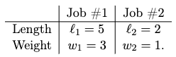
where the first job would have a larger ratio, so GreedyRatio would schedule it first, but GreedyDiff would schedule the second job first. But we realize that the weighted completion time:
- for GreedyRatio is $3 \cdot 5 + 1 \cdot 7 = 22$
- for GreedyDiff is $1 \cdot 2 + 3 \cdot 7 = 23$ is worse!
So we can rule out GreedyDiff, and we are left with GreedyRatio. But is GreedyRatio correct? Luckily in this case it is!
Theorem: Correctness of GreedyRatio. For every set of positive job weights $w_1, w_2, …, w_n$ and positive job length $l_1, l_2, … , l_n$, the GreedyRatio algorithm outputs a schedule with the minimum possible sum of weighted completion times.
Proof: we will use exchange arguments. The key idea is prove that every feasible/alternative solution can be improved by modifying it to look more like the output of the greedy algorithm $\implies$ the greedy algorithm is optimal.
Without loss of generality, let us compute the ratio for every job $j$ and renumber the jobs such that:
\[\frac{w_1}{l_1} \ge \frac{w_2}{l_2} \ge ... \ge \frac{w_n}{l_n}\]so that $\sigma$ is the sequence $[1,2, … , n]$. Suppose by contradiction that we have some competitor $\sigma^{}$ that is better, and $\sigma^{} \neq \sigma$. For the greedy output we get essentially:
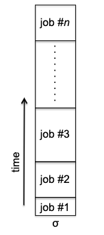
but note that for any other schedule, we will have a consecutive inversion: a pair of job $i > j$ (so $j$ has a higher score) such that job $i$ is processed immediately before job $j$. For instance $\sigma^{‘}$ has a consecutive inversion:
| $\sigma^{*}$ | $\sigma^{‘}$ |
|---|---|
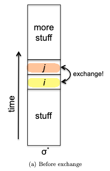 |
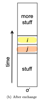 |
Lemma: Non-Greedy Schedules Have Inversions. Every schedule $\hat{\sigma}$ different from the greedy schedule $\sigma$ has at least one consecutive inversion.
- proof: if $\hat{\sigma}$ has no consecutive inversion, then the index of each job is at least 1 larger than the job that came before. Since there are only $n$ jobs and the maximum index is $n$, the jump between two consecutive job must be 1. Then $\hat{\sigma}$ must be the same as $\sigma$.
Now, the key idea is to perform an exchange from $\sigma^{*}$ (to reach $\sigma^{‘}$) and realize it can only perform at least as good. After the swap above of job $i,j$, we realize that:
- the objective does not change for the jobs before $i$ and after $j$
- for job $i$ in $\sigma^{*}$, it went up in $\sigma^{‘}$ so the cost increased by $l_{j} \cdot w_i$
- for job $j$ in $\sigma^{*}$, it went down in $\sigma^{‘}$ so the cost decreased by $l_{i} \cdot w_j$
But since $i > j$ by construction ($j$ had a higher score), it means:
\[\frac{w_i}{l_i} \le \frac{w_j}{l_j} \implies l_{j} \cdot w_i \le l_{i} \cdot w_j\]So $\sigma^{‘}$ is at least as good as $\sigma^{}$, with $\sigma^{‘}$ being more ordered = more similar to $\sigma$! More precisely, we can show that $\sigma^{‘}$ has exactly one less inversion than $\sigma^{}$. To see this, define an inversion to be a pair $k,m$ of job such that $k < m$ (so $k$ has a higher score) but $m$ is schedules before $k$, AND that they need not be consecutive. Then, realize that swapping one consecutive inversion does not change the relative order of $k,m$ relative to each other or $k,m$ relative to $i,j$:
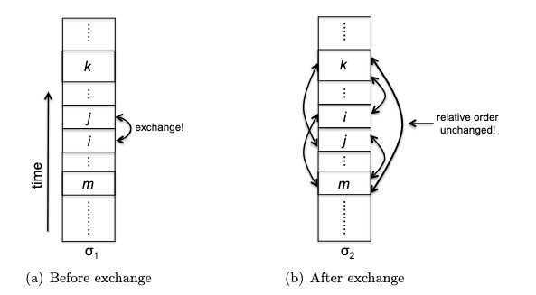
In other words, restoring consecutive inversion doesn’t affect any other inversions (if any). Therefore, this means:
- having one less consecutive inversion produces a schedule at least as good!
- having one less consecutive inversion also decreases the total number of inversion by one
Therefore, we can repeatedly swap jobs to remove consecutive inversions until we get $\sigma$, which has no inversions. During the process, the objective function can not increase ($\le$). Hence $\sigma$ is at least as good as any $\sigma^{*}$ along the way. This means that $\sigma$ is optimal, and we are done.
Huffman Codes
Huffman coding is a widely-used method for lossless compression. For example, every time you import or export an MP3 audio file, your computer uses Huffman codes. This section will cover the optimality of Huffman codes, and a fast algorithm for computing them.
Compression Task: consider an input “string” that consists of symbols from an alphabet $\Sigma$ (e.g. a set of 64 symbols including all 26 letters plus punctuations and some special characters). Your goal is to represent this string to a binary code, i.e. a sequence of 0s and 1s, so that the code is as short as possible while still being able to recover the original string.
Note that there are two different tasks here:
- encoding: find a mapping that maps each symbol to a binary code
- decoding: given a binary code, can recover the original string without ambiguity
For instance, consider the following alphabet to encode:
\[\Sigma = \{ A,B,C,D \}\]and consider the following two encoding schemes:
| fixed-length code | variable-length code |
|---|---|
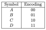 |
 |
While variable code in general can be shorter if designed correctly (so we will focus on this), but in this case what would the string “001” decode to? Note that this issue does not arise with fixed-length codes since we know where to start and end for each symbol. With variable-length codes, we must impose a constraint to prevent ambiguity.
Prefix-Free Codes
We can eliminate all ambiguity by insisting that a code is prefix-free. This means that given any two pair of distinct symbols $a,b \in \Sigma$, the encoding of $a$ is not a prefix of that of $b$, and vice versa.
With a prefix-free code, encodings are unambiguous
Why? If, say, the first 5 bits of a sequence match the encoding of a symbol $a$, then $a$ was definitely the first symbol encoded. Because the code is prefix-free, there’s no way these 5 bits could correspond to (a prefix of) the encoding of any other symbol.
An example of prefix-free code would be fixed length code, or the following variable-length code:
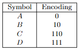
But how do we find a variable-length code that is also prefix-free? Crucial to reasoning about the problem is a method of associating codes with labeled binary trees. This is most easy to see with examples:
| Encoding | Tree |
|---|---|
 |
 |
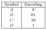 |
 |
 |
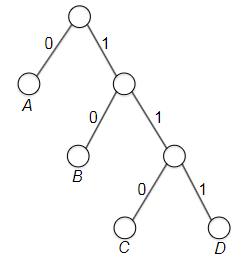 |
where essentially edges are the encoding, and vertices are potential symbols. Notice that
- every binary code can be represented as a binary tree with left and right child edges labeled with “0” and “1,” respectively, and with each symbol of the alphabet used as the label for exactly one node
- the number of edges in a path/depth equals the number of bits used to encode the corresponding symbol
But more importantly:
- In general, the encoding of a symbol $a$ is a prefix of that of another symbol $b$ if and only if the node labeled $a$ is an ancestor of the node labeled $b$.
- therefore, because no leaf can be the ancestor of another, a tree with labels only at the leaves defines a prefix-free code (i.e., no label will be parent)
Finally, we can visualize decoding as traversing the tree until we hit a leaf, and restarting from the root. For example, given the input string “010111” and the tree below, we would decode it as “ABD”:
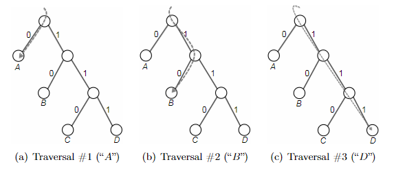
Huffman’s Greedy Algorithm
Now that we have a way to represent a prefix-free code as a binary tree, we can formulate the problem as follows:
Task: Optimal prefix-free code. Given a string to encode, with each symbol $a \in \Sigma$ having a frequency $p_a$, our objective is to minimize:
\[\min_T \sum\limits_{a \in \Sigma} p_a \cdot \text{depth}(a)\]where $T$ is a binary tree with labels only at the leaves, which would define any prefix-free code.
Now since we can have symbols of different frequency, it becomes apparent that variable length prefix-code is what we are looking for: associate the most frequent symbols with the shortest codes/number of bits.
The overall idea is to consider a bottom-up algorithm. We start with every symbol $a \in \Sigma$ as a leaf, and then we will repeatedly merge some symbols until we get a tree. But what do we choose which ones to merge in order to minimize the objective?
Intuition: labels with high frequency are costly so they should be at the top of the tree. Hence, we should keep small frequency labels at the deeper levels.
So, the idea for greediness is to consider merging ‘‘symbols’’ with the smallest frequencies first (bottom-up). i.e. every iteration of Huffman’s greedy algorithm myopically performs the merge that least increases this objective function.
Why could it possibly be a good idea? Realize that each merge increments the depths of all the leaves in the two participating trees and, hence, the encoding lengths of the corresponding symbols:
| Before Merge | After Merge |
|---|---|
 |
 |
where technically you are merging two trees (or two root nodes) each time, and specifically for every leaf/symbol in the two trees after merging, the depth increases by 1. This causes the objective function to increase by:
\[\sum\limits_{a \in T_1} p_{a} + \sum\limits_{a \in T_2} p_{a}\]because for symbol has increased one more bit, but as it appears $p_a$ times,the total cost increases $p_a$ for each leaf. Huffman’s greedy criterion thus dictates that we merge the pair of trees for which the sum above is as small as possible.
The pseudo code thus look like:
def huffman(S):
  # S is a set of symbols with frequencies p_a
  # initialize a forest of trees, one for each symbol
  F = { Tree(a, p_a) for a in S }

  while len(F) > 1:
    T_1, T_2 = two_trees_with_smallest_freq(F)
    # merge them into a new tree
    T_3 = merge(T_1, T_2)  # root of T1, T2 become the children of a new internal node
    T_3.p_a = T_1.p_a + T_2.p_a  # invariant: for every internal node, its p_a is the sum of its children

    F.remove(T_1)
    F.remove(T_2)
    F.add(T_3)
  return the only tree in F
Before proof of correctness, consider a quick example. Given input of
and each iteration of the algorithm looks like:
- initialize with 4 trees, each with a single symbol
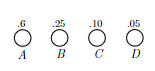
- smallest is node C and D:
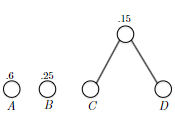 merge and obtain a new subtree with root CD at cost of $0.10+0.05=0.15$
 - smallest two are $0.15$ and $0.25$, so merge the subtree CD with B:
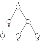 and obtain a new subtree with cost $0.4$
 - Finally
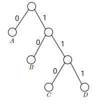 where if we take the left edge to represent 0 and the right 1, this returns a variable length prefix-free code of A=0, B=10, C=110, D=111.
Correctness of Huffman’s Algorithm
Now we want to show that the encoding returned by the above greedy algorithm is correct. In general greedy algorithm is not easy to prove, and here we will use induction + exchange argument to prove it.
Before the proof, we first notice that the algorithm is iteratively committing two smallest $p_a$ symbols $a,b$ to be siblings in the final tree. Therefore the plan is to show that:
- Huffman’s tree is the best (minimizes the average leaf depth) amongst all possible trees in which $a$ and $b$ are siblings
- there is an optimal tree in which $a$ and $b$ are siblings
Visually, each iteration of the algorithm is like:

and to prove that the output tree is optimal (combining claim 1 and 2) we need to show that:
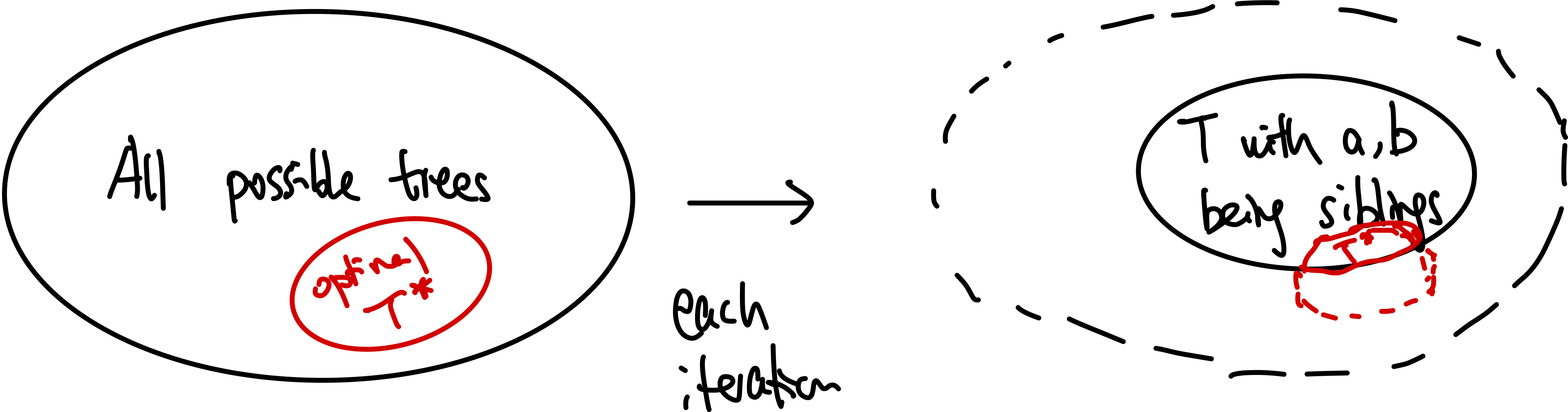
If we can prove both of the above, then we are basically done (by induction).
Proof by induction. Let us denote $P(k)$ be the statement that Huffman’s tree output the best with an alphabet size at most $k$.
- base case: when $k=2$, there is only a tree with one root and two leaves. So Huffman’s tree is optimal.
- inductive hypothesis: assume $P(k’)$ is true for $k’ < k$.
-
inductive step: we need to show that $P(k)$ is true. Since each step of the algorithm we are merging two least frequent “symbols” (the root of the subtree), we want to show claim 1 and claim 2 to hold in order to prove that the output tree at this stage is optimal.
Proof for claim 2: we begin by first showing that there is an optimal tree in which $a$ and $b$ are siblings. To prove this, we will use the exchange argument again. Consider some arbitrary tree $T$, and without loss of generality, denote a sibling at the lowest level of the tree as $x,y$. Let $a,b$ the nodes with the smallest frequency $p_a$. We want to show that the objective function/cost is at least as good as the one with $a,b$ as siblings.
Consider changing the $a,b$ and $x,y$ pair:
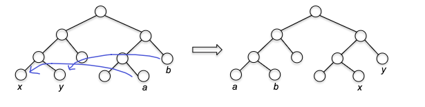
Then notice that the new tree $T’$ changed cost function by:
\[\begin{align*} \Delta L &= \underbrace{p_{a} (\mathrm{depth}(x) - \mathrm{depth}(a)) + p_{b} (\mathrm{depth}(y) - \mathrm{depth}(b))}_{\text{cost}} \\ &+ \underbrace{p_{x} (\mathrm{depth}(a) - \mathrm{depth}(x)) + p_{y} (\mathrm{depth}(b) - \mathrm{depth}(y))}_{\text{benefit}} \\ \end{align*}\]which we can simplify to
\[\Delta L = (p_{a} - p_{x}) \cdot (\Delta(x,a)) + (p_{b} - p_{y}) \cdot (\Delta(y,b))\]where by definition of $x,y$ being the deepest we know that $\Delta(x,a) \ge 0$ and $\Delta(y,b) \ge 0$. Additionally, since by construction $p_a, p_{b} \le p_x, p_y$, we know that $\Delta L \le 0$ after the exchange, so the cost is at least as good $\implies$ there exists an optimal tree with $a,b$ being siblings.
Proof of Claim 1: We will use induction to show that Huffman’s tree is the best amongst the sibling trees $T_{ab}$ where $a,b$ being the least frequent symbol are siblings. The trick is that we can do induction proof on $\Sigma’$-tree, where each step of the algorithm we “rename” the symbols instead of denoting them as subtree (e.g. merging $a,b$ gives the new symbol $ab$). Then note that the tree constructed in this notation is essentially the same as tree constructed in the original notation with $\Sigma$:
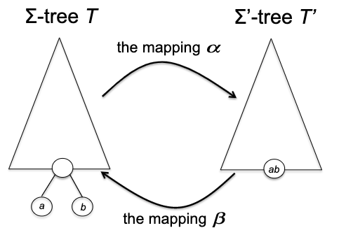
with the only difference being $p_{ab} = p_a + p_b$, and the average leaf depth is the same up to a constant that is independent of the choice of the tree:
\[L(T) = L(T') + p_a + p_b\]because the expanded tree has node $a,b$ being one level deeper. Now, we can very easily show that running Huffman on $\Sigma’$ (replacing $a,b$ with $ab$ and $p_{ab} = p_{a} + p_{b}$) using the induction hypothesis we left off earlier. Since now $\vert \Sigma’\vert < \vert \Sigma\vert = k$, Huffman algorithm returns the optimal tree $T’_{ab}$ for $\Sigma’$-tree.
Then, because each $\Sigma’$-tree correspond to $\Sigma$-tree (with $a,b$ being siblings) and the average leaf depth is preserved (up to a constant), then knowing an optimal tree in $\Sigma’$-tree, is knowing an optimal in $\Sigma$-tree with $a,b$ being siblings.
where RHS is what we just proved, and LHS is claim 1.
Combining claim 1 and claim 2, the induction step is complete because by claim 1, Huffman outputs the best-possible tree from the restricted $T_{ab}$ set and by claim 2, such a tree $T_{ab}$ must be optimal.
Running Time of Huffman Algorithm
The simple implementation would run in $O(n^{2})$, because we will merge in total $n-1$ times for $n = \left\vert \Sigma\right\vert$ , and each iteration needs to identify the two smallest trees in the forest, which takes $O(2n)$ time by simple scan. There, however, is a small change we can make it run a bit faster:
Heap: a special Tree-based data structure in which the tree is a complete binary tree.
- Min-Heap: the key present at the root node must be minimum among the keys present at all of it’s children. The same property must be recursively true for all sub-trees in that Binary Tree.
- Max-Heap: the key present at the root node must be maximum among the keys present at all of it’s children. The same property must be recursively true for all sub-trees in that Binary Tree.
and the key usage is that deleting the top element of the heap or the highest priority element, and then re-balancing the tree only takes $O(\log N)$. (Actually it is $O(H)$ for $H$ being the height of the tree, which is $\log N$ if it is a complete binary tree). Therefore each find min/find max operation takes $O(\log N)$ time.
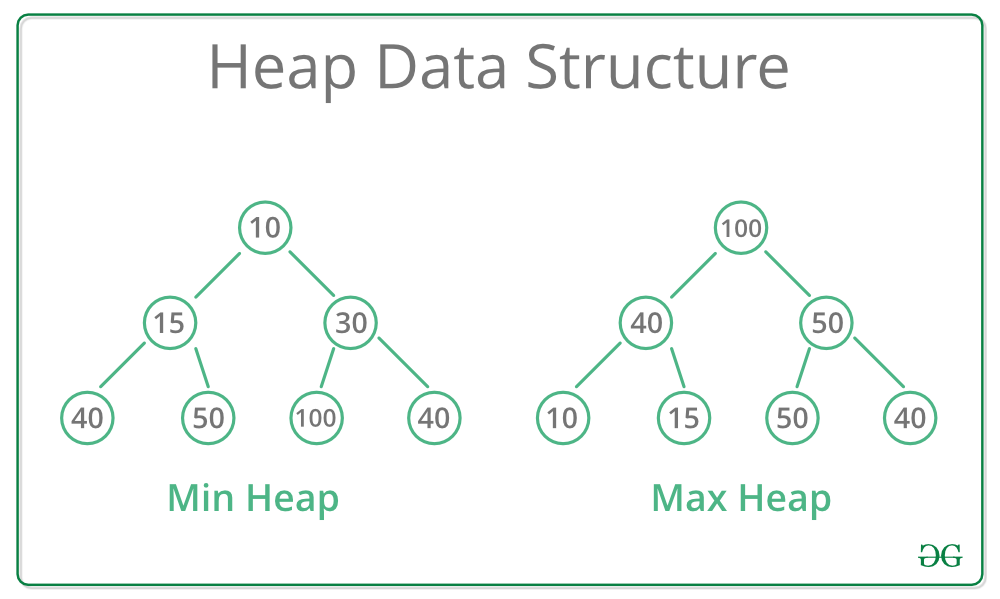
Therefore, since we are repeatedly finding the minimum, we can use a min-heap to store the nodes/symbols, and then each iteration we can delete the top two elements and insert the new node, which takes $O(\log n)$ time. Therefore, the overall running time is $O(n \log n)$.
Minimum Spanning Trees
The MST problem is a uniquely great playground for the study of greedy algorithms, in which almost any greedy algorithm that you can think of turns out to be correct. The goal is to find, in a given graph $G= (V,E)$ with weight $w$ on edges, what is the best subset of edges $T \subseteq E$ such that the resulting graph with $T$ will:
- spanning: connect every vertex in $V$ (i.e. one connected component)
- tree: it is a spanning tree: there are no cycles.
- minium: it has the minimum total weight
Minimum Spanning Tree Problem. Input undirected graph $G=(V,E)$ in which each edge $e$ has a real-valued cost $c_e$, and the goal is to output a minimum spanning tree $T \subseteq E$ of $G$.
- note that it would only make sense if $G$ is a connected graph, otherwise there is no spanning tree.
For example, the red highlighted is a MST with cost $7$:
Prim’s Algorithm
The algorithm closely resembles Dijkstra’s shortest-path algorithm, except that we have no ‘‘source vertex’’ and we are trying to find a spanning tree rather than a shortest-path. The idea is to greedily pick the cheapest edge that cross the frontier until done (starting from any random vertex).
So an example before we going to the pseudo code:
| iteration 1 | iteration 2 | iteration 3 |
|---|---|---|
 |
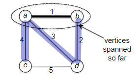 |
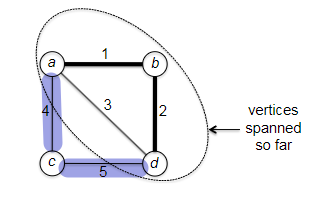 |
where we started from vertex $b$, and at each iteration we checked the all edge that cross the “frontier” and picked the cheapest one. The pseudo code is:
def prim(G):
  # G is a connected graph with edge weights w
  # initialization
  X = {s}  # s is an arbitrary vertex
  T = []  # output and also an INVARIANT: edges that span X

  while X != V:
    # find the cheapest edge (u,v) with u in X, v not in X
    e = (u,v) = cheapest edge with u in X, v not in X
    T.add(e)
    X.add(v)
  return T
where :
- one obvious implementation could give $O (mn)$ since you are looping over all vertices once (n times) and finding the cheapest edge (m times) for loop.
- we will first show that this indeed outputs a MST
- and then we will also see that the algorithm is correct no matter which vertex it chooses to start from
Correctness of Prim’s Algorithm
Proving the correctness of Prim’s algorithm is a bit easier when all the edge costs are distinct (this is to just make the proof easier, the algorithm is still correct without it), and let us take that as an assumption for now.
To prove this, we consider showing two things:
- Prim outputs a tree (with no cycles)
- The tree is spanning and minimal.
- first show that every edge picked by Prim satisfies the “minimum bottleneck property”
- then we show that a spanning tree with only MBP edges is a MST
Proof for claim 1: consider a generic graph $G$ that can have multiple connected components. Then consider adding one edge $(u,v)$:
- Type 1: if $u,v$ already in the same CC:
- this will create a cycle (because there was already path from $u$ to $v$)
- number of CC remains the same
- Type 2: if $u,v$ in different CC:
- this will not create a cycle
- number of CC decreases by 1
to visualize this:
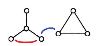
where having the red edge will create a cycle, and the blue will not. Now, notice that in Prim’s algorithm, we will 1) start with $n$ distinct CCs, 2) add $n-1$ edges to the graph, and 3) finish with one CC. Therefore, every edge added must be type 2, and hence the output is a tree (graph with no cycle).
Note that the above also proved the statement: if $T \subseteq E$ has only $n-1$ edges AND the resulting graph is connected, then $T$ must be a tree.
Proof for claim 2: we need to first define the MBP property, prove that Prim’s algorithm only picks MBP, and finally prove that a tree with only MBP edges is a MST.
Minimum Bottleneck Property: an edge $(u,v) \in E$ with cost $c_{uv}$ satisfies the MBP if and only if there is no $u \overset{p}{\leadsto} v$ path that consists solely of edges with cost less than $c_{uv}$.
- i.e. for any other path you can think of, there is at least one edge that is more expensive than $(u,v)$
For example, in the following graph, edge $(a,d)$ does not satisfy MBP, but edge $(a,c)$ does:
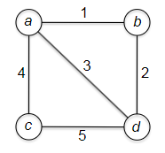
Now, we prove that Prim’s algorithm only picks MBP edges. The trick is to realize that any path (see below) $v^{} \leadsto w^{}$ will have at least one edge that crosses the frontier. Since Prim picks the cheapest such edge, all other path must have at least one edge that is more expensive than the one picked by Prim.
To see this more concretely, consider the same argument as from Dijkstra’s proof. Consider an edge $(v^{}, w^{})$ chosen in an iteration of Prim’s algorithm, with $v^{} \in X$ and $w \notin X$. Now, consider any arbitrary path $v^{} \overset{p}{\leadsto} w^{*}$:

Note that since $w^{*} \notin X$, at some point the path will go inside the frontier to the outside. Let that happen with edge $(x,y)$ crossing the frontier in that path. However, since Prim guaranteed:
\[c_{v^{*}w^{*}} \le c_{xy}\]for every edge $(x,y)$ that crosses the frontier. Now, since this means there is at least one edge on any other path that will exceeded $c_{v^{}w^{}}$, we know that $(v^{}, w^{})$ satisfies the MBP.
Finally, we need to show that a tree with only MBP edges is a MST. To show this, we consider by contradiction that there is a MST $T^{*}$ that does not have the MBP property all the way but still has the minimum cost.(shown in solid lines):
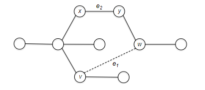
Let Prim’s tree be $T$. Since $T \neq T^{}$, there is at least one MBP edge, e.g. $e_1=(u,v)$, that is not in $T^{}$. Since $T^{}$ is a tree, there exists a path $u \overset{p}{\leadsto} v$. But since $e_1$ is an MBP edge, this means there exists an edge $e_2$ on $u \overset{p}{\leadsto} v$ that has cost *higher than $e_1$. Now, consider an exchange argument that:
- we add $e_1$ to $T^{*}$. This is a type 1 edge and will create a cycle and does not increase the number of CC (still one)
- Remove $e_2$ from $T^{*}$. Since you are removing an edge from the cycle, this is undoing type 1 edge and also does not increase the number of CC (still one)
Now, we obtain $T’$:
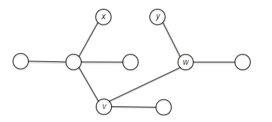
where by the above argument, $T’$ has also just $n-1$ edges and is connected $\implies$ $T’$ is a valid spanning tree. However, since $\mathrm{cost}(e_1) \le \mathrm{cost}(e_2)$ by MBP, then cost of $T’$ is less than $T^{}$, which is a contradiction. Therefore, every edge in $T^{}$ must satisfy MBP to be MST, and hence Prim’s $T$ is a MST.
Note: from HW 5, you can also show that the converse is true: every edge on a MST must satisfy MBP.
- this does not imply your MST will include every $(u,v)$ edge that is MBP, because having $u,v$ being connected in your MST may not even require having a $u\to v$ edge).
Running Time of Prim’s Algorithm
The obvious runtime we discussed is $O(nm)$, but notice that it was repeatedly doing extract min. This hints at using a heap data structure.
Recall: (min-)Heap: a special Tree-based data structure in which the tree is a complete binary tree, such that you can
inserta new node with (key, value) pair into the tree,extract_minto get the node with the smallest key and rebalance the tree, anddeleteto remove a node from the tree and rebalance the tree. The treeordersnodes by the keys, and all of these operations take $O(\log n)$ time.
- how? a short peek into the implementation is that you either percolate up or percolate down the tree to rebalance it
- e.g. fo insert, you add the new node at the bottom, and then percolate up (swap with parent if this is smaller until done). Since the height of the tree is $O(\log n)$, this takes $O(\log n)$ time.
To use heap for Prim, since we are repeatedly picking the minimum cost edge that crossed the frontier, we want the heap to:
- Invariant 1: only store edges that cross the frontier
- Invariant 2: for each $v \notin X$, we will always keep $\mathrm{key}(v)=$ cheapest edge $(u,v)$ that crosses the frontier with $u \in X$. If no such edge exist for a node, store $\infty$.
For example, invariant 2 would look like:
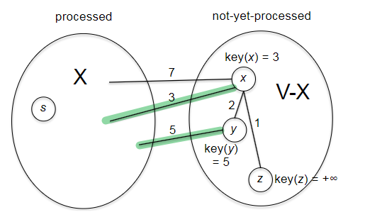
If the above two invariant hold for every iteration of our implementation, then it is obvious that taking the minimum from such heap $\implies$ cheapest edge amongst the cheapest for each nod $\notin X$ $\implies$ the cheapest edge that crosses the frontier.
How to we keep the two invariants? Invariant 1 hold easily because after we extract_min we removed the $(u,v)$ from the heap $\iff$ that $v$ was outside $X$ is now inside the frontier. So it is automatically satisfied. But after extract_min, e.g. we took vertex $x$ from the above image to $X$, some of the $\mathrm{key}(v)$ might need to be updated (e.g. that of vertex $z$). But note that since our frontier only changed by that newly added vertex, we only need to update keys related to that vertex! Specifically, we need to:
# w* is just extracted

# for every edge from w* that crossed the frontier
for every edge (w*, y) with y not in X:
    # update the new min cost for y = key(y)
    if c_w*y < key(y):
      delete y from heap
      key(y) = c_w*y
      best_edge(y) = (w*, y)
      insert y into heap
Now, the full algorithm looks like:
def prim_w_heap(G):
  X = {s}  # s is an arbitrary vertex
  T = []  # output and also an INVARIANT: edges that span X
  H = heap()  # heap of edges that cross the frontier

  # initialization
  for v in V and v != s:
    # for every edge that crosses the frontier s
    if (s,v) in E:
      key(v) = c_s*v
      best_edge(v) = (s,v)
      insert v into H
    else:
      key(v) = inf
      best_edge(v) = None

  # main loop
  # if H is empty, then there is no vertex NOT in X = we are done!
  while H is not empty:
    # extract the cheapest edge that crosses the frontier
    w* = extract_min(H)
    T.add(best_edge(w*))  ##### greedy choice
    X.add(w*)

    # update the keys for every edge from w* that crossed the frontier
    for every edge (w*, y) with y not in X:
      # update the new min cost for y = key(y)
      if c_w*y < key(y):
        delete y from heap
        key(y) = c_w*y
        best_edge(y) = (w*, y)
        insert y into heap
  return T
So what is the runtime of this?
- initialization phase performs does $n-1$ heap insert (i.e. once for every vertex not $s$), and $O(m)$ additional work as it checks the edges. So this takes $O(n \log n + m)$ time.
- the main while loop goes for $n-1$ iterations, and inside it at least does extract mins. This is already $O(n \log n)$. But additionally, notice there is also a for loop. However, realize that each edge of $G$ will enter this for loop exactly once, at the time when first of its endpoints get sucked into $X$. Therefore, since there are $m$ edges, this will give in total for the entire algrithm $O(m \log n)$.
Hence adding up we get:
\[O((n+m) \log n) = O(m \log n)\]since for a connected graph $G$, the least number of edges is $m \ge n-1$. Therefore, you can simplify the above to $O(m \log n)$.
Kruskal’s Algorithm
Why this in addition to Prim?
- provides an opportunity to study a new and useful data structure, the disjoint-set or union-find data structure.
- there are some very cool connections between Kruskal’s algorithm and widely-used clustering algorithms
Similar to Prim, this algorithm is greedy. Different from Prim’s algorithm which grows a single tree from a starting vertex, Kruskal can grow multiple trees in parallel, and coalesce into a single tree only at the end of the algorithm.
Idea: repeatedly (greedily) pick the cheapest edge that does not create a cycle, until done.
For example:
| iteration 1 | iteration 2 | iteration 3 | iteration 4 |
|---|---|---|---|
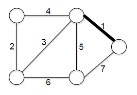 |
 |
 |
 |
where we started with $T$ being empty, and at each iteration we picked the cheapest edge that does not create a cycle. The pseudo code is:
def kruskal(G):
  # G=(V,E) with costs c_e for each e in E
  T = []  # output
  sorted_edges = sort(E)  # sort edges by increasing cost
  for e in sorted_edges:
    if adding e to T does not create a cycle:
      T.add(e)
  return T
note that similar to Prim, it requires a connected undirected graph $G=(V,E)$ with edge weights $c_e$ for each $e \in E$.
A straight-forward runtime for this algorithm is:
\[O(m \log m) + O(m n) = \log(m \log n) + O(mn) = O(mn)\]where:
- $O(m \log m) = O(m \log n)$ because we know $m \le n^{2}$, hence $O(\log m) = O(2 \log n)$. This equality will be used later as well
- $O(mn)$ because you can search for cycles in $O(m)$ time using DFS/BFS (this is equivalent to checking if the new edge $e=(u,v)$ are already reachable).
Before we discuss how to make this faster using union-find, we need to first prove that this algorithm is correct. Without prior context, it is hard to see why this produces a tree that spans all vertices.
Correctness of Kruskal’s Algorithm
This section proves Kruskal’s algorithm is correct, under the simlar assumption that all edge costs are distinct (this is to just make the proof easier, and does not affect the algorithm’s correctness).
It is obvious that Kruskal produces no cycles, but we need to show that:
- the output is connected
- the output is a spanning tree
- the output is minimal (by achieving MBP)
Proof for Claim 1: Consider $T$ be the set of edges chosen by Kruskal so far, and that in this iteration Kruskal just finished examining an edge $e = (v,w)$. Then in the algorithm:
- if $v,w$ are already in the same CC, then adding $e$ will create a cycle, so this is skipped
- otherwise, $(v,w)$ is added to $T$, fusing their CCs into one
Therefore, just after this $(v,w)$ will be in the same CC. Since this is true for every iteration, we know that at the end of the algorithm, all vertices (since it will check all edges and the input graph is connected) will be in the same CC, and hence the output is connected.
Proof for Claim 2: since the algorithm explicitly ensures that the output is acyclic, and we just showed that all its vertices belong to the same CC, then it is a tree.
Proof for Claim 3: We prove by contrapositive, that Kruskal never includes an edge that is NOT MBP. To show this, consier an edge not being a MBP, and we want to show that Kruskal’s algorithm will never include it.
Let $e=(v,w)$ be not a MBP. Then there exists a path $v \overset{p}{\leadsto} w$ that consists solely of edges with cost less than $c_{vw}$. Because Kruskal scans through (greedily) the edges in non-decreasing cost, all edge of $P$ will be checked before $e$. From claim 1, we know that once an edge $e’=(x,y)$ is checked, both $x,y$ are in the same CC. Therefore, when we reached $e=(v,w)$, we know that $v,w$ are already in the same CC, and hence adding $e$ will create a cycle. Therefore, Kruskal will never include $e$.
Visually, by the time we are checking the black $e$ edge, we would have checked all the blue edges:
Speeding up Kruskal with Union-Find
Prim’s algorithm is sped up using a genric data structure called heap, and Kruskal can also be sped up using a data structure called union-find.
Union-Find Data Structure: the goal is to maintain a partition of a static set of objects. This is often used to efficiently track and manipulate connected components or disjoint sets. It supports the following operations:
Initialization: create a new union-find data structure with $n$ objects ($O(n)$)Union: given two objects form a (different) union, merge the two sets into a single setFind: determine which set a given object belongs to
note that (though not used by Kruskal), with a good implementation the Union and Find operations both take time logarithmic in the number of objects. Since Kruskal itreatively checks connected components (if there is a cycle) and grow them, we can visualize the process as:
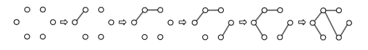
such that finding if two vertices are in the same CC is just checking if they have the same root in a union. So instead of a DFS/BFS, we could just have done it in $O(1)$ by comparing if the two vertices have the same root! But how does union-find work?
Quick-and-Dirty Implementation of Union-Find.
The datastructure can be implemented by an array, where each index position represent a vertex $v \in V$, and stores the parent vertex (e.g., a root vertex representing the CC).
| Implementation | Visualization |
|---|---|
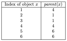 |
 |
where in the drawing, the green vertices and edges are the original graph. The black circle highlights the ‘‘leader’’ representing this CC, and the red edges represent which vertex is the parent of which. This red graph is sometimes also called the parent graph.
With the notion that it stores the parent graph, the rest is easy:
initialize: for each $i=1,2,3, … , n$, initialize $parent[i] = i$ (i.e. each vertex is its own parent)- therefore, this takes $O(n)$ cost
find: given a vertex $v$, repeatedly check $parent[v]$, until $parent[v] = v$ (i.e. $v$ is its own parent).- therefore, this takes $O(\mathrm{depth})$ of the parent tree
unionpick the union $x$ that has a larger size (with the parent keep a fieldsize), and let the other union be $y$. Find the root of both unions, let them be $i,j$. Then set $parent[j] = i$ and update thesize.- if we don’t merge the smaller one with the larger one so that our size at least doubles, we cannot get the logarithmic runtime
- if we don’t merge with the root node, then the depth of vertices in $y$ will increase by more than one, impacting runtime. Visually for
unionif done o non-root node:
Now, we can implement Kruskal’s algorithm in $O((m+n) \log n)$ time. The idea is to:
- the parent pointer all point to the root of a CC, so that finding the root is $O(1)$. This means checking if two vertices are in the same CC is $O(1)$.
- to maintain the above invariant, when an edge $e=(u,v)$ is picked, merge all members of the smaller union into the larger union. Note that this is not $O(n)$ for each merge:
- each vertex can only be called to be merged/updated $\log_{2}$ times since each merge at least double the size.
- since there are in total $n$ vertices, the total cost in the entire algorithm is $n \log n$.
So finally we get preprocessing $O(m \log n)$, cycle check $O(m)$, and union update $O(n \log n)$, which gives $O((m+n) \log n)$.
Clustering
We will show that one application of Kruskal’s algorithm is to solve a problem called clustering. The goal is to partition a set of objects into a collection of clusters, such that given $n$ data points, they are classified into a coherent group:
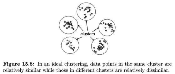
to do this, we assume that we are given:
- a distance measure $d(p,q)$ between each pair of data points
- a distance measure being symmetric
- we’ve decided to get to $k$ clusters
There are many ways to do this (e.g. bottom-up, top-down, k-means). Here we discuss bottom-up or agglomerative clustering is to begin with every data point in its own cluster, and then successively merge pairs of clusters until exactly $k$ remain.
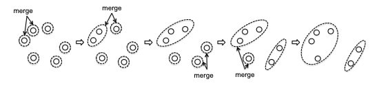
so the key part is how to decide which two clusters to merge at each step.
Here we discuss one way to do it: single-link clusering, where we are optimistic such that we consider two clusters to be similar if their closest points are close. Formally, let the similarity measure between two clusters being $F$, then:
\[F(S_1, S_2) = \min_{p \in S_1, q \in S_2} d(p,q)\]Therefore our single-link bottom up clustering algorithm is:
def bottom_up():
  while C contains more than k clusters:
    C1, C2 = closest pair of clusters in C
    remove C1 and C2 from C
    add C1 union C2 to C
  return C
note that one advantage of bottom-up algorithm is that during the process of running this, you also get the result for all $k' < k$!
Connection to Kruskal’s Algorithm: recall that in kruskal we “merge” two vertices if they are the smallest edge and are in different CC. This has great similarilty to merging two clusters if the simialrlity function checks the best pair of points from each cluster. In fact, the two are exactly the same except that in Kruskal does not stop at $k$
- define a complete undirected graph $G=(X,E)$ from the dataset $X$, such that $E$ represent every pair of points in $X$, and the edge costs are $d(p,q)$
- run kruskal on $G$ until $k$ connected components, return the tree $(X,T)$
- compute the connected components of $(X,T)$, which is the clustering result
Introduction to Dynamic Programming
Most people initially find dynamic programming difficult and counterintuitive. However, this is relatively formulaic hence can be learned with practice. In this section, we are getting warmed up with some simple examples.
Weighted Independent Set
First, some terminologies
Independent Set: a subset of vertices $S \subseteq V$ such that no two vertices in $S$ are adjacent. More formally, every $v,w \in S$ has $(v,w)\notin E$.
For example, in the two graphs below
| Graph 1 | Graph 2 |
|---|---|
 |
 |
- the first graph has six independent sets: $\emptyset$ and five singletons
- the second has the same six independent sets that the complete graph does, plus some (five) independent sets of size two. In total eleven.
Weighted Independent Set Problem: given an undirected grpah $G=(V,E)$ and a non-negative weight $w_v$ for each vertex $v \in V$, find an independent set $S \subseteq V$ of maximum total weight (of the vertices).
- the solution is also called a maximum-weight independent set (MWIS)
- e.g., if vertices represent courses, vertex weights represent units, and edges represent conflicts between courses, the MWIS corresponds to the feasible course schedule with the heaviest load (in units)
This is quite a difficult problem even if we just consider path graphs to be $G$
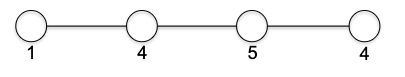
where by looking at it we can see the solution is $8$.
- if we do exhaustive search, notice that there are 8 independent sets. This will grow exponentially (consider adding one more vertex to the path graph, and think about how many more independent sets you will have).
- if we do greedy, maybe consider simply start picking from the largest vertex (i.e., with weight 5). Immediately you got the wrong answer.
- if we do divide-and-conquer is natural if we can break this into smaller subproblems. So we can consider maybe recursively computing MIS of the left half, the right half, and merge? But the problem is how do we merge to keep the independence?
Linear-Time Algorithm for WIS in Path Graph
Insight: the trick for DP is to consider how an optimal solution must be constructed in a prescribed way from optimal solutions to smaller subproblems, and vice versa
This feels very similar to divide-and-conquer, so here I hightlight the difference (from stackoverflow):
- DnC:
- dividing the problem into sub-problems, conquer each sub-problem independently and combine these solutions.
- Most of the canonical applications of the divide-and-conquer paradigm replace a straightforward polynomial-time algorithm
- DP:
- solving problems with overlapping subproblems. Each sub-problem is solved only once and the result of each sub-problem is usually stored in a table (generally implemented as an array or a hash table) for future references.
- The killer applications of dynamic programming are polynomial-time algorithms for optimization problems for which straightforward solutions (like exhaustive search) require an exponential amount of time.
WIS in Path Graph Problem. Consider $G=(V,E)$ being a $n$-vertex path graph with edges $(v_1, v_2), (v_2, v_3), …, (v_{n-1}, v_n)$ and a non-negative weight $w_i$ for each vertex $v_{i} \in V$. Find an independent set $S \subseteq V$ of maximum total weight (of the vertices).
Suppose we are given an optimal solution MWIS $S \subseteq V$ with total weight $W$. What can we say about $S$? What can we say about the solution to a smaller subproblem given $S$?
The trick to this problem is that $S$ either contains the last vertex $v_n$ or doesn’t. We have two cases:
- $v_n \notin S$. Then let $G’ = G$ without $v_n$. This would mean that:
- the set $S$ is also an independent set in $G’$, and since $S$ is the MWIS in $G$, then $S$ is also the MWIS in $G’$.
- we can show the above (MWIS for $G’$) by contradiction: if there is $S^{}$ that is MWIS for $G’$ with weight larger than $S$, then this means $S^{}$ would also be an independent set with larger weight than $S$ in $G$, which is a contradiction.
in other words, if you know MWIS for $G’$ and you know $v_n \notin S$, then you can just use the MWIS for $G’$ as the MWIS for $G$.
- $v_{n} \in S$. Then since $S$ is an indepednt set, we know that the penultimate vertex is not there.
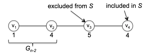 Therefore, we can consider $G’’$ to be $G$ without $v_n$ and $v_{n-1}$. Then we can show that:
- $S - {v_n}$ is an independent set for $G’’$, and since $S$ is the MWIS in $G$, then $S - {v_n}$ is also the MWIS in $G’’$.
- again can be proven by contradiction using a simlar logic as above.
in other words, if you know MWIS for $G’’$ and you know $v_n \in S$, then you can just use the MWIS for $G’’$ as the MWIS for $G$.
The upshot of the above analysis is that now you have a recipe for building UP a solution from subproblems: Let $S$ be an MWIS for $G$ with at least two vertices, and the nwe can find $S$ must be either
- an MWIS for $G’=G_{n-1}$ (i.e. without $v_n$)
- an MWIS for $G’‘=G_{n-2}$ plus $v_n$
where $G_i$ denote the subgraph comprising its first $i$ vertices.
So all we need to do is to solve small problem, and then build up. Now how do we implement this?
Naive Recursive Approach from divide-and-conquer. Since the best solution is either of the two, we can just try both and return the max!
def recursive_mwis(G):
  if G has no vertices:
    return 0
  elif G has one vertex:
    return {v1}
  else:
    # case 1: MWIS for G' without v_n
    mwis1 = recursive_mwis(G without v_n)
    # case 2: MWIS for G'' without v_n and v_{n-1}
    mwis2 = recursive_mwis(G without v_n and v_{n-1}) + v_n
    return max_weight(mwis1, mwis2)
This is guaranteed to be correct using proof by induction and the property of $S$ we just proved. But what is the runtime? Exponential!
- each recursive call only throws away one or two vertices, so there are $O(n)$ height in the recursion tree (compared to the ‘correct’ DnC ones, there were only logarithmic height)
- since the branching factor is 2, this gives $O(2^{n})$ number of leaves!
The key difference now, between DP and DnC is that DP could avoid a lot of computation by memoizing the results of subproblems. Why is this related in this context? Consider how many distinct subproblem did the recursive algorithm solve?
- since each subproblem is defined by the input graph, this is equivalent to how many distinct graphs we are solving
- the answer is $n+1$ since each time we are removing graphs from the tail! (empty graph, $G_1$, …, $G_n$).
Therefore, we could cache the results of each subproblem, and then we can just look it up when we need it. This is called memoization. Implementation-wise, we can just use an array, where $A[i]$ represent the MWIS of $G_i$. However to really see the runtime speed up, the more direct way is to build from bottom up.
def wis(G):
  A = [] * (n+1) # solutions for n+1 subproblems
  A[0] = 0
  A[1] = w1
  for i in range(2, n+1):
    A[i] = max(A[i-1], A[i-2] + wi)
  return A[n]
note that now:
- this is DP
- this is clearly linear time
- but it only returns the maximum weight, not the vertices themselves. Therefore a common step after DP is a postprocessing *reconstruction algorithm*
- though you can hack this
wisto also let $A$ store the vertices of an MWIS of $G_i$, the reconstruction algorithm is more genreally memory and time efficient
- though you can hack this
Reconstruction Algorithm (MIS)
Typically when you have a DP, you would have a reconstruction algorithm easily defined based on the same principle as the algorithm you came up with.
Consider back to the question: is $v_{n}$ included in the solution? Since we know $A$, we can actually answer this question immediately by looking at $A[n-1]$ and $A[n-2]$:
- if $A[n-1] \ge A[n-2] + w_n$, then $v_n$ is not in the solution. Continue the process with thinking about $v_{n-1}$
- otherwise, $v_n$ is in the solution. Continue the process with thinking about $v_{n-2}$
therefore the reconstruction algorithm is:
def wis_reconstruction(G, A):
  # A is the array we computed from `wis`
  S = [] # the solution
  i = n
  while i >= 2:
    if A[i-1] >= A[i-2] + wi:
      i -= 1
    else:
      S.add(v_i)
      i -= 2
  if i == 1:
    S.add(v_1)
  return S
wich is like doing a single backward pass, which runs in $O(n)$ to get us the real solution.
Note: the full MWIS problem on arbitrary graph is NP-complete. Even though we know that from HW 6, the following relation hold for arbirary graph:
\[W_{G} = \max\{W_H, W_K + w_v\}\]where $G$ is the
'originalgraph, $H$ is the graph without $v$, $K$ is the graph without $v$ and $v$’s neighbor, and $w_v$ is the weight of $v$. So why does not NOT lead to linear time algorithm? The number of times you will need to lookup a subproblem’s solution is NOT constant!
Principles of Dynamic Programming
The above example showcase a paradigm in DP:
DP Paradigm: we begin by thinking about the optimal solution if we are given the optimal solution of smaller problems (and vice versa). Then:
- identify a relatively small number of subproblems (otherwise the runtime will be exponential)
- show how to quickly and correctly solve a larger problem using the solutions to a small number of subproblems
- quickly and correctly infer the final solution from the computed subproblem solutions (e.g. reconstruction algorithm)
More specifcally, DP under this paradigm would be fast if we consider the runtimes:
\[\underbrace{f(n)}_{\text{\# subproblems}} \times \underbrace{g(n)}_{\text{time/subproblem}} + \underbrace{h(n)}_{\text{postprocessing}}\]where $f(n),g(n), h(n)$ would come from point 1,2,3 mentioned above, respectively. In the case of WIS, we have:
- $f(n) = n$ since there are $n+1$ subproblems
- $g(n) = O(1)$ since each subproblem is just a constant time comparison
- $h(n)=O(n)$ is the backward reconstruction cost
so the total runtime is $O(n)$ for our WIS example.
The Knapsack Problem
The next example is the Knapsack problem, which follows closely to the paradigm we just discussed.
Knapsack Problem: consider $n$ items with value $v_1, …, v_n$ and sizes $s_1, …, s_n$, all being positive integers. Consider you have a knapsack with capacity $C$, and you want to maximize the total value of items you can put in the knapsack.
For example, given the following configuration, the maximum value you can stuff in is 8 for a capacity of 6:
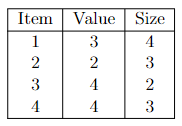
Now we can kind of just copy over the idea for WIS we had. Again, suppose someone gave you the optimal solution $S \subset {1,2,3 ,…,n }$ telling you the best items to put in the knapsack. We can we say about $S$ and problems of smaller size? Either $S$ includes the last item $n$ or it doesn’t.
- $n \notin S$. Since the the optimal solution $S$ excluded it, the solution $S$ must also be feasible and optimal for the knapsack of size $C$ and items $1,2,3,…,n-1$.
- $n \in S$. First of all, this only happens if $s_{n} \le C$. Then what happens if we remove $n$? The solution $S - { n}$ is an optimal solution for the knapsack of size $C - s_n$ and items $1,2,3,…,n-1$. Notice the difference with
wis:- both case in
wisconsider both subproblems by knocking out vertices. - here, we need to change both size and items
- both case in
But regardless, this gives us a recipe of how to build up a solution from subproblems. Again writing down the recurrence: let $V_{i,x}$ denote the maximum total value for a subset of the first $i$ items with total size at most $c$. Then:
\[V_{i,c} = \max \begin{cases} V_{i-1, c} \\ V_{i-1, c-s_i} + v_i, & \text{only if } c \ge s_i. \text{ otherwise it will be $V_{i-1, c}$} \end{cases}\]So what are the subproblems we need to solve in this case? $V_{i,c}$ for all $i \in {0,1,2, …, n}$ and $c \in { 0,1,2, …, C }$. Another way to see this is that now we have two parameters to specify input for each subproblem. Therefore it is natural that now we are filling up a 2D array
def knapsack(V,S,C):
  A = (n+1) * (C+1) array  # 2D array for solutions to subproblems
  for c in range(0, C+1):
    A[0,c] = 0  # base case

  for i in range(1, n+1):
    for c in range(0, C+1):
      if c >= s_i:
        A[i,c] = max(A[i-1, c], A[i-1, c-s_i] + v_i)
      else:
        A[i,c] = A[i-1, c]

  return A[n,C]
Runtime? Obviously $O(nC)$ since we are filling up a 2D array.
Reconstruction? Again, a backward pass to figure out from $A[n][C]$ which case (whether $n$-th item is included) it is:
- if $A[n-1][C] = A[n][C]$, then obviously $n$ is not included and we continue to $A[n-1][C]$
- otherwise, then $n$ is included and we continue to $A[n-1][C-s_n]$
def knapsack_reconstruct(A, C):
  S = [] # the solution
  c = C
  for i in range(n, 1, -1):
    if A[i-1][c] != A[i][c]:
      S.add(i)
      c -= s_i
    # else we are skipping i, capactiy is the same
  return S
which runs in $O(n)$. Visually it is doing this:
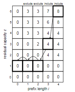
Finally, correctness. In general this will be proven by induction + the property we used to come up with the DP algorithm/recurrence itself. Hence, we omit the proof here.
Advanced Dynamic Programming
In this section we will discuss some more advanced DP problems, where the structure of optimal solution is more complex than that of the last section.
Sequence Alignment
This problem is both used in computational genomics and in NLP (e.g. to compute the edit distance). Consider the input consist of strings (e.g. representing portions of genomes) over some alphabet:
\[\text{Input: AGGGCT},\qquad \text{Output: AGGCA}\]and the goal is to say “how similar the two strings are”. How do we measure similarity?
Alignment: a way of inserting gaps such that the two strings have the same length. For example:
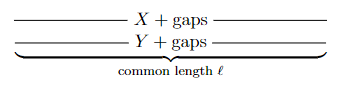
so that then we can define the similarity of the two strings as the quality of the best alignment, for example
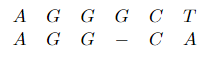
Finding Optimal Sequence Alignment then is used to answer the question “how similar the two strings are”. Formally, consider two strings $X,Y$ over the alphabet $\Sigma$. And let there be a penalty $\alpha_{xy}$ for swapping $x$ with $y$, and $\alpha_{\mathrm{gap}}$ be the cost of inserting a gap. The goal is to find an optimal alignment of $X,Y$ that minimizes the total penalty.
- intuitively, is saying “how similar are the two strings” = “most plausible explanation” of how one of the strings might have evolved into the other.
- the minimum penalty of an aligmment is famous enough as a concept that it has a name: Needleman-Wunsch or NW score.
So how do we solve it? Consider some alternative, e.g. greedy algorithm. If you give enough thought, you will realize that it is impossible because you really need to think ahead to avoid bad choices early on, which is the opposite of greedy.
The savior is again dynamic programming. Similar to prior approaches, we begin by reasoning about how optimal solution relates to optimal solutions of subproblems, and vice versa. Consider we are already given the optimal solution, and similar to previous problems, consider the subproblem is having one less character to align:
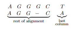
This naturally becomes similar to WIS and Knapsack, but here we could have more cases. Let the optimal alignment for $X= x_1, x_2, …, x_m$ and $Y= y_1, y_2, …, y_n$ be given above. Denote $X’ = x_1, x_2, …, x_{m-1}$ and $Y’ = y_1, y_2, …, y_{n-1}$ both with last one removed:
-
Case 1: $x_m$ is aligned with $y_n$, two actual characters (may or may not be the same). Then you can peel them off and the rest of the alignment should also be optimal:
\[P' + \alpha_{x_m y_n} < P + \alpha_{x_m y_n}\]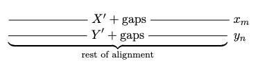 note that this alignment between $X’$ and $Y’$ will also be the optimal aligmnent. (Proof by contradiction: suppose that the penalty for this induced alignment of $X’, Y’$ is $P$, but there is another better competitor $P’ < P$. Then appending $x_m, y_n$ to the competitor alignment gives back $X,Y$, with new cost:
which is a contradiction that $P + \alpha_{x_m y_n}$ was the optimal alignment.) Note that $\alpha_{x_m y_n}$ could be zero.
- Case 2: $x_m$ is aligned with a gap. Then the induced alignment of $X’,Y$ is optimal.
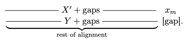
- Case 3: $y_n$ is aligned with a gap. Then the induced alignment of $X,Y’$ is optimal.
- Case 4: a gap with a gap. Note that this is not a scenario, as we could have removed both gaps. Therefore, in general, any column/pairing in an alignment will be either of the three cases above.
Now we can build a recurrence relation: since the optimal solution must be either one of the three cases, and each case either removes a character from $X$ or $Y$, we can write the recurrence as:
\[P_{m,n} = \min \begin{cases} P_{m-1, n-1} + \alpha_{x_m y_n} \\ P_{m-1, n} + \alpha_{\mathrm{gap}} \\ P_{m, n-1} + \alpha_{\mathrm{gap}} \end{cases}\]since this must be true for every $n=1,2, …$ and $m=1,2, …$ we get more generally from bottom-up:
\[P_{i,j} = \min \begin{cases} P_{i-1, j-1} + \alpha_{x_i y_j} \\ P_{i-1, j} + \alpha_{\mathrm{gap}} \\ P_{i, j-1} + \alpha_{\mathrm{gap}} \end{cases}\]for every $i=1,2, …$ and $j=1,2, …$ representing the subproblem of aligning first $i$ symbols in $X$ with first $i$ symbols in $Y$. Finally, what if one of $i,j$ is zero? This is the base case: imagine $X$ of the $X,Y$ is empty, then the alignment cost will be $\alpha_{\mathrm{gap}} \vert X \vert$. So we obtained:
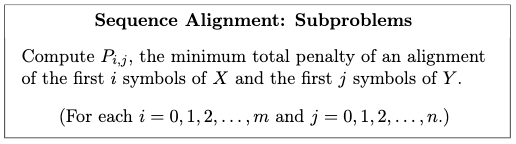
which means our algorithm would be progresively filling in a 2D array:
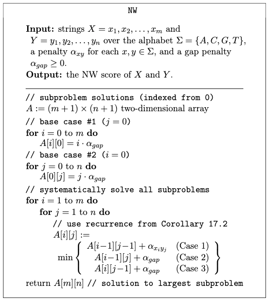
which obviously has a runtime of $O(nm)$.
Proof of correctness? Induction on $i+j$ (the subproblem size), with the recurrence relationship justifying the inductive step.
How do we reconstruct it? Start from the top $A[m][n]$ and figure out which of the three cases it went into. This can be done by checking A[i-1][j-1], A[i-1][j], A[i][j-1] and see which one it is. Then we can continue to that case and repeat. Details omitted here but this will be $O(n+m)$ since each time you are decreasing at least one of the two numbers $i,j$ by one.
Optimal Binary Search Trees
Goal: compute the best-on-average search tree given stastistics about the frequencies of different searches. Recall that the defining property of search tree is
Search Tree Property: for every object $x$
- object in $x$’s left subtree must have keys smaller than $x$
- object in $x$’s right subtree must have keys larger than $x$ (assuming no duplicate keys for simplicity)
This means that visually we are dealing with a fast search datastructure that looks like:
for every subtree in the search tree. An example would be:
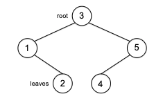
Average Search Time
Normally, when we consider a binary search tree, we measure the search time for a key $k$ to be the nunmber o nodes it need to visit while searching for $k$ (including $k$ itself). For exmaple in the following tree:
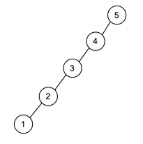
key “1” wold have a search time 5. Therefore, without weights, the ideal search tree would be a balanced one
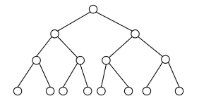
because this would minimize the length of the longest root-leaf path, or equivalently, the maximum search time. Minimzing the maximum search time makes sense since you don’t have knowledge about which searches are more likely than others.
However, here we consider the problem
Optimal Binary Search Trees: A sorted list of keys $k_{1} < k_{2} < … < k_n$ and nonnegative frequency $p_i$ for each key $k_i$. We want to minimize the weighted search time:
\[\sum_{i=1}^n p_i \times \text{search time for } k_i = \sum_{i=1}^n p_i \times (1 + \mathrm{depth}_T(k_i) )\]where $\mathrm{depth}_T(k_i)$ represent the depth of $k_i$ in the tree $T$. (The root will be considered as depth zero.)
This looks very similar to the optimal prefix-tree code problem, where the goal is to also related to find a tree to minimize the average (weighted) depth. However, the challenge here is that, in the prefix-free code problem, the only restriction is that symbols appear at leaves, but here we have the search tree property. This makes greedy algorithm not work in this problem. Similarly divide-and-conquer algorithm would also struggle (imagining recursively choosing a root node to be the median, and continue). Fundamentally this is because the choice of root has unpredictable repercussions further down the tree if you chose too early.
So how do we do it? Different from other previous problems, there is no clear notion of the rightmost/last object to pluck off and obtain optimal thing for subproblem. But the intuition is that we can imagine building the tree from bottom up, and imagine the last decision we have to make = determing the root node!. Consider, if we know the optimal solution is the following
Then we (intuitively) also
- know the optimal solution for keys $1, ..., r-1$ and $r+1,. .., n$ will be $T_1, T_2$. (see proof below)
- the key is IF we know "what $r$ is"
- recall that in WIS, we know the rest of the solution if we know “whether the last vertex is included or not”
- recall that in Knapsack, we know the rest of the solution if we know “whether last item is included or not”
- therefore, the smaller subproblem is the trees $T_1, T_2$, and the case analysis will be all the possible roots.
Proof: Let the root of $T$ have key $r$ (same as figure above). We want to show that the residents of $T_1$ with $p_1, …, p_{r-1}$ is optimal, and similarly for $T_2$ with $p_{r+1}, …, p_n$.
Suppose by contradiction that one of the subtrees, e.g. $T_1$ is NOT an optimal solution, so that we have a search tree $T_1^*$ that achieves a better search time with the same keys:
\[\sum\limits_{k=1}^{r-1} p_{k} \cdot (k\text{'s search time in $T_1^{*}$}) < \sum\limits_{k=1}^{r-1} p_{k} \cdot (k\text{'s search time in $T_1$})\]Then intuitively, we want to show that we can cut and paste this tree into $T$ and the obtain a cost better than $T$:
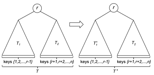
where RHS is the one we cut and pasted. The weighted search time of the original tree $T$ is:
\[\begin{align*} & p_{r} + \sum\limits_{i=1}^{r-1} (1 + 1 + \mathrm{depth}_{T_1}(k_i) ) + \sum\limits_{j=r+1}^{n} (1 + 1 + \mathrm{depth}_{T_2}(k_j) ) \\ &= \sum\limits_{i=1}^{n} p_i + \sum\limits_{i=1}^{r-1} (1 + \mathrm{depth}_{T_1}(k_i) ) + \sum\limits_{j=r+1}^{n} (1 + \mathrm{depth}_{T_2}(k_j) ) \\ &= \sum\limits_{i=1}^{n} p_i + \text{weighted search time of $T_1$} + \text{weighted search time of $T_2$} \end{align*}\]since the first and third term is the same for the weight time in $T^{}$, and we know that $T_1^{}$ is better than $T_1$, this is a contradiction to the statement that $T$ was optimal.
From the above observation, we obtain the recurrence relationship that, llet $W_{i,j}$ denote the weighted search time for keys ${i, i+1, …, j}$, then:
\[W_{1,n} = \sum\limits_{k=1}^{n} p_{k} + \min\limits_{r \in \{1,2, ..., n\}} \left( W_{1,r-1} + W_{r+1,n} \right)\]where $W_{1,n}$ is the full problem, and $W_{1,r-1}, W_{r+1,n}$ are the subproblems. Notice that this also implies solving the subproblems (recursively) must be a dealing with a contiguous chunk of keys = a subtree. Since for the search tree property to hold, the above must be true for every subtree:
\[W_{i,j} = \sum\limits_{k=i}^{j} p_{k} + \min\limits_{r \in \{i,i+1, ..., j\}} \left( W_{i,r-1} + W_{r+1,j} \right)\]where intutively, $W_{i, i}$ would representing you building a search tree with just the root node $r=i$. Then, the algorithm would just iteratively grow this tree like this:
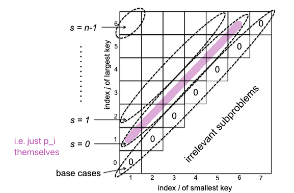
Alternatively you can also just start with the purple diagonal as base case in your algorithm, and go to the top left. And you will fill each new diagional from bottmo left to top right (think about why by looking at the recurrence relation).
and the detailed algorithm would be:
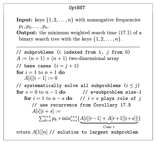
where the runtime would be:
- there are $O(n^2)$ subproblems
- each subproblem does a min over $O(n)$ choices
so the total runtime is $O(n^3)$ (though with some optimization, you can get to $O(n^{2})$)
Shortest Path Revisited
This chapter considers a DP approach for computing the shortest path in a graph. Both are slower than Dijkstra or Prim’s algorithm, but:
- Bellman-Ford can deal with negative edge weights and can be done in a distributed manner
- Floyd-Warshall can also deal with negative edge weights and can compute shortest-path distance between any pair of vertices
Shortest Path with Negative Edge Length
As mentioned before, Dijkstra algorithm ca nfail with graphs that has negative edges (but not negative cycles). The reason is the greedy decision it makes now doesn’t work. Consider:
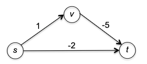
where the shortest path from $s \leadsto t$ will be $s \to t$ in the first iteration of Dijkstra, which is wrong.
In general (for any graph that may have negative edges or cycles):
- if you have a negative cycle, then any shortest distance doesn’t make sense as its $- \infty$
- What if in the presence of a negative cycle you forbidden that option for your optimal path? This version where no repeat vertices is allowed of the single-source shortest path problem is actually a NP-hard problem.
Therefore, in this section we will consider the revised problem
Shortest Path Revised: given a directed graph $G=(V,E)$ with edge lengths $l_e$ for each edge $e \in E$, and a source vertex $s \in V$, either:
- If there is a negative cycle, then the algorithm should report it and done.
- Otherwise, compute the shortest path distance $d_v$ from $s$ to every other vertex $v \in V$.
However, if there is no negative cycle, then there are a few properties we can exploit to help us reach a solution quickly:
If a graph has no negative cycle, the optimal path $s \leadsto v$ must contain at most $n-1$ edges/cannot contain repeated vertices.
Proof: consider an optimal path $P’$ that has at least $n$ edges. This means it visits at least $n+1$ vertices, meaning some vertex $w$ is visited twice. This means we can splice the repeated part out from $P’$ while keeping thee same endpoints but with fewer edges now:
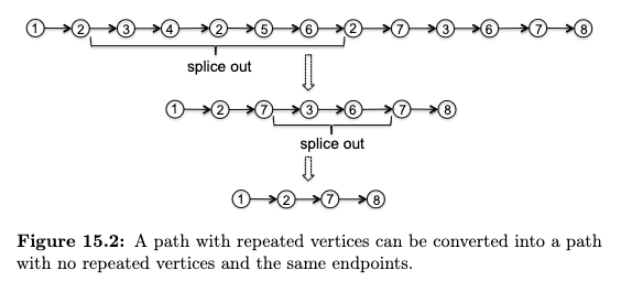
But because there is no negative cycle, this spliced out (path) cycle must have nonnegative length. Therefore, the new path $P’’$ is shorter than $P’$, which is a contradiction.
Bellman-Ford Algorithm
Again, the most important step is to reason about the optimal solution: what are the different ways that an optimal solution might be built up from optimal solutions to smaller subproblems?
Naively, you may think of subproblems being something based on a subset of the $G$ we need to solve (e.g., similar to how we solve WIS, where input graph is a path graph and we just pluck the last vertex out). However, the problem now is that where is the “last vertex” in a generic graph? Bellman-Ford thus considers a different approach. Although there is no sequentiality in input graph, there is sequentialality in output graph, i.e., the optimal path:
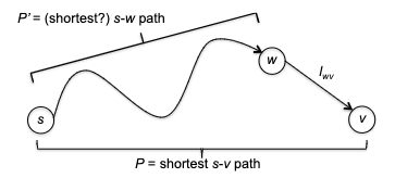
which we will show that $P’$ must also be shortest (even if $w \to v$ can ve negative). This is great, but what is the subproblem?
Bellman-Ford Subproblem: we only consider (optimal) paths that use less than $i$ edges each time. More formally, let the input graph be $G=(V,E)$ with a given source vertex $s \in V$. Consider finding the optimal $P$ bewteen $(s,v)$ that includes at most $i$ edges.
- note that different from previous DP, each subproblem here still work on the full input
How does this help construct an optimal solution to a larger problem? Consider the following:
- that optimal $P$ for $s \leadsto v$ has at most $i-1$ edges (already a pretty good path using a budget $i-1$). Then $P$ must also be the optimal solution with edge budget $i-1$ for $s \leadsto v$. (Proof by contradiction: if not, then that shorter path would also be shorter for the original subproblem of at most $i$ edges.)
- that optimal $P$ uses exactly $i$ edges. Consider visually that optimal path and $P’$ being the last edge plucked (say $(w,v)$):
 then that $P’$ is an $s \leadsto w$ optimal path with at most $i-1$ edges (a smaller subproblem BUT with different destination). This can be easily shown by contradiction as well, because if there exists a better path with at most $i-1$ edges from $s \leadsto w$, then we can swap that out and obtain a better $P$ to the original problem.
Therefore:
- we can construct an optimal $P$ for the budget of $i$ using the “two” cases above
- but how many subsoluions will the original subproblem need to look at? Consider computing the optimal path $s \leadsto v$ with cost $i$. Then “case 1” is one candidate, and “case 2” would have $\text{in-degree}(v)$ candidates. So in total it will scan through $1+\text{in-degree}(v)$ candidates.
Anyway, this gives use the recurrence relationship. Let $L_{i,v}$ denote the minimum length of an $s\leadsto v$ path with at most $i$ edges, cycles allowed (since we have an edge budget, even negative cycles could be fine in this definition for now). Then for every $i \ge 1, v \in V$:
\[L_{i,v} = \min \begin{cases} L_{i-1, v} \\ \min\limits_{(w,v) \in E} \left( L_{i-1, w} + l_{wv} \right) \end{cases}\]if no such path exist, then $L_{i,v} = \infty$. But when should we stop $i$?
Bellman-Ford Convergence: interestingly, we can show that $L_{i,v}$ will converge if for some $k \ge 0$:
\[L_{k+1,v} = L_{k,v} \qquad \forall v \in V\]then this would mean:
- $L_{k’,v} = L_{k,v}$ for every $k’ \ge k$ and any destination $v$
- for every destination $v$, then $L_{k,v}$ must be the $\mathrm{shortest}(s,v)$ in $G$
Proof for statement 1: Because $L_{k+1,v} = L_{k,v}$, then this means the subproblem of $L_{k+2}$ is doing
\[L_{k+2,v} = \min \begin{cases} L_{k+1, v} \\ \min\limits_{(w,v) \in E} \left( L_{k+1, w} + l_{wv} \right) \end{cases} = \min \begin{cases} L_{k, v} \\ \min\limits_{(w,v) \in E} \left( L_{k, w} + l_{wv} \right) \end{cases} = L_{k+1,v}\]Thus, any future subproblem will be the same as $L_{k+1,v}$, which is the same as $L_{k,v}$ by assumption.
Proof for statement 2: if $L_{k,v}$ is NOT the shortest path for subproblem with at most $k$ edges. Then the shortest path must be beyond $k$ edges. This is a contradiction since we know that $L_{k’,v} = L_{k,v}$ for any $k’ \ge k$ if the assumption holds.
Bellman-Ford Stops with No Negative Cycles: if there ARE negatiev cycles in the graph, then the condition $L_{k+1,v} = L_{k,v}, \forall v \in V$ in general will not even happen. But if there are no negative cycles, then it will converge exactly when reached $n-1$ edge budget (i.e., every vertex used in the path):
\[L_{n,v} = L_{n-1,v} \qquad \forall v \in V\]the contrapositive statement of this is also powerful:
\[\text{no neg cycle means convergence} \implies \text{not converging means has neg cycle}\]so this algorithm can also detect negative cycles.
Why? Remeber we showed that in Section Shortest Path with Negative Edge Length, the optimal $s \leadsto v$ path in a graph with no negative cycle must at most visited every vertex once (otherwise we could remove the cycle and get a shorter path). Therefore, this is the only place where we need the no-negative cycle condition, such that Bellman-Ford’s algorithm will stop/converge at $n-1$ iterations. If not, then there is a negative cycle:
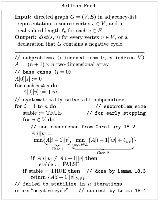
where again, we needed to fill up a 2D array because we have two parameters, $i,v$ for the subproblem.
Proof of Correctness: induction on $i$, with our recurrence relationship justifying the inductive step.
Runtime: Superficially it looks like $O(n^{2})$ loops with $O(n)$ to compute the recurrence relation in the inner most loop. However, realize that during the “for $v\in V$” loop we actually just did:
\[\sum_{v \in V} \text{in-degree}(v) = m\]abd in the outer for loop over $n$ iterations, we thus only need $O(nm)$ time! (if the graph is dense, then $m=O(n^{2})$ so we get the same solution as our naive analysis).
Floyd-Warshall Algorithm
Now we can deal with all-pairs shortest path:
All-Pairs Shortest Path Problem: consider a directed graph $G=(V,E)$ with a real-valued length $l_e$ for each edge. The goal is to:
- find the shortest path distance $\mathrm{shortest}(u,v)$ from every vertex $u$ to every other vertex $v$.
- if there is a negative cycle, then the algorithm should report it and done.
Technically, we could solve this using Bellman-Ford by treating every vertex as source vertex. This will give us $O(n^{2}m)$ runtime, with potentially $m=O(n^{2})$. We show that we can do better than this by finishing in $O(n^{3})$.
The trick here is to still look at the output paths, and also puts some contraint on length. However, we further restrict the identity of the vertices that can go into the solution.
Floyd-Warshall Subproblem: First we label each vertex $v\in V$ with names ${1,2,3, …, n}$. Then, consider the shortest path from $v$ to $w$ that only uses vertices in ${1,2, …, k}$ as intermediate vertices. i.e. this minimum path
- begins at $v$ and ends at $w$
- the path (excluding $v,w$) only includes vertices in ${1,2, …, k}$
- does not contain a directed cycle (by assuming there is no negative cycle so that we can splice out any cycle out of a path and end up with a lower cost.)
- We shall also see how negative cycles can be detected later
Let $L_{k, u, v}$ denote the length of this path. If no such path exists, then $L_{k, u, v} = \infty$. Note that you can therefore imaging subproblem size defined by $k$: for a fixed origin-destination pair $v,w$, the set of allowable path will grow by $k$ and the minimum cost will only decrease.
For example:
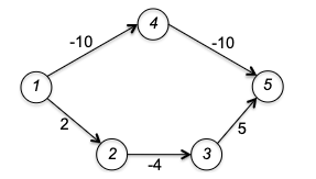
In this graph, if we had source and vertex being $1,5$, then if $k=0,1,2$ there is no feasible path so $L_{k,1,5}=\infty$. However, when $k=3$, then the path $1 \to 2 \to 3 \to 5$ is eligible (and being the only one) with cost $L_{3,1,5} = 3$.
This we will soon see will make the optimal solution naturally break down into only two smaller subproblems. Suppose $P$ is a $v \leadsto w$ with no cycles and only uses vertices in ${1,2, …, k}$ as intermediate vertices. Then realize that that $P$ can either use the lastly added vertex $k$ or not:
- Case 1: optimal $P$ for $v \leadsto w$ did NOT use $k$ as an intermediate vertex. Then $P$ must be an optimal path with at most $k-1$ intermediate vertices as well. (Proof by contradiction)
-
Case 2: optimal $P$ for $v \leadsto w$ did use $k$. Then we can split the path into two by removing $k$ to be uneligible:

because $k$ could have only appeared in $P$ once (by assumption of cycle-free optimal path), then $P_1$ is optimal with origin $v$ and destination $k$, and $P_2$ is optimal with origin $k$ and destination $w$, both with a smaller subproblem using only ${1,2, …, k-1}$ vertices.
- to prove that $P_1, P_2$ is also optimal is slightly tricky here. Suppose there is a better $P_1^{}$ for $v \leadsto k$. To concatenate $P_1$ with $P_2$ we want to have a lower cost than $P$ to get a contradiiction.
- If $P_1^{*}$ with $P_2$ will have no cycle, proof done.
- If $P_1^{}$ with $P_2$, denote $P^{}$, now has a cycle, we need to invoke the assumption that there is no negative cycle in $G$. Therefore we can splice up the cycle in $P^{}$ such that we still hhave the same origin $u$ and destination $v$ in now a cycle free path $\hat{P}$, which can only be shorter than $P^{}$.
- to prove that $P_1, P_2$ is also optimal is slightly tricky here. Suppose there is a better $P_1^{}$ for $v \leadsto k$. To concatenate $P_1$ with $P_2$ we want to have a lower cost than $P$ to get a contradiiction.
In sum, we broke the large problem into “two” subproblems: case 1 is reducing the problem size by one, and case 2 is reducing the problem size by one AND changing the source/destination pairs.
Therefore, suppose (for now) $G$ has no negative cycles. Then the recurrence relation is deinfed by letting $L_{k,v,w}$ be the minimum length of a cycle-free path from $v$ to $w$ that only uses vertices in ${1,2, …, k}$ as intermediate vertices. Then:
\[L_{k,v,w} = \min \begin{cases} L_{k-1, v, w} \\ L_{k-1, v, k} + L_{k-1, k, w} \end{cases}\]which has to be true for every $k \in {1,2, …, n}$ and every $v,w \in V$.
Finally this gives the algorithm:
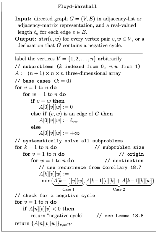
where note that:
- since we are viewing subproblems defined by size $k$, the base cases are $L_{0,v,w}$. This can result in three cases:
- if $v=w$, then $L_{0,v,w}=0$
- if $(v,w) \in E$, then $L_{0,v,w}=l_{vw}$
- otherwise $L_{0,v,w}=\infty$
- since the subproblems grows by $k$, the outermost loop will start with $k$
- this algorithm can detect negatiev cycles as well (see below why)
Proof of Correctness: induction on $k$, with our recurrence relationship justifying the inductive step.
Runtime: $O(n^{3})$ since we are filling in a 3D array, and each subproblem takes $O(1)$ time to compute.
Detecting Negative Cycles
What if the input graph has a negative cycle?
Lemma 18.8: the graph $G$ has a negative cycle if and only if, at the conclusion of the algorithm, there is a vertex $v$ such that $L_{n,v,v} < 0$.
Proof: if there is no negative cycle, then obviously $L_{n,v,v} = 0$ for every $v$ since every shortest path will also be cycle free. But if there is a negative cycle, then this means $G$ has a negative cycle with no repeated vertices other than its start and end (e.g. $v$). The trick is to think about two paths to form such a cycle, and argue how a repeated vertex can be spliced out.
Let $C$ denote such a cycle, and let $k$ be the largest labeled vertex of $C$ with $k \neq v$:
then we know:
- $P_1, P_2$ are cycle-free $v \leadsto k$ and $k \leadsto v$ paths respectively (since this cycle has no repeated vertex other than source) with vertices restricted to ${1,2, …, k-1}$
- then Floyd-Warshall would found $L_{k-1, v, k}$ and $L_{k-1, k, v}$ to be at least smaller or equal to the actual length of $P_1, P_2$ (being cycle-free)
- therefore, $L_{k,v,v}$, which is at most the length $L_{k-1, v, k} + L_{k-1, k, v}$, will also be smaller or equal $C$, which is negative.
Therefore, if there is a negative cycle, $L_{k,v,v}$ will at least once become negative. This means $L_{n,v,v}$ will be negative since for each iteration $k’ > k$ the minimum length only decreases.
Max Flows and Min Cuts
Before we dive into the algorithms, its sometimes enlightening to see how those seemingly “unrelated/unpractical” algorithms can be very useful in practice. Here we will see two examples.
Minimum Cut Problem
Minimum Cut Problem: consider a flow nertwork consisting of a directed graph $G=(V,E)$ with a source vertex $s$ and a sink vertex $t$. Each edge $e \in E$ has a capacity $c_e$. The goal is to find a $(s,t)$ cut into two sets $A,B$ such that it minimizes the total capacity of edges sticking out from set $A$ into $B$.
\[\min \sum_{e =(u,v); u \in A, v \in B} c_e\]
- basically think of those source and sink as water flows, and the capacity is the pipe
- the cut is basically coming up with two groups of vertices but one needs to include $s$ and the other needs to include $t$.
Visually, a cut below would be optimal with a total capcity of 3:
where:
- the purple edge would not count as it is not flowing from $A$ to $B$
- the green edge will count
- the blue edge would not count as it is flowing from $B$ to $A$
Notice that since this is just choosing which vertex goes where, there are $2^{n-2}$ possible cuts (excluding source and sink). We will not see an algorithm here, but we will see how this can be solved in linear time in the next section.
Minimum Cut Application: Image Segmentation
We will see how this minimum cut problem relates to how we can do image segmentation. First we formalize the “version” of image segmentation we are considering:
Image Segmentation with Fore/background: Consider the task of classifying pixels of an image to be either foreground or background. Let us be given some prior (e.g. heuristics, non-negative) that each pixel could be in foreground with $a_v$ and background with $b_v$. Additionally, we are given non-negative $p_e$ for each undirected edge between each pixel, which represents the fact that we want neighboring pixels to be close together, i.e. smooth.
Then, we can define the segmentation as an undirected graph with all those costs/rewards assigned to the vertices and edges:
where the first value of the nertex denotes $a_v$ and second denotes $b_v$ in this example. We want to maximize the objective:
\[\max_{(X,Y)}\quad \sum_{v \in X} a_v + \sum_{v \in Y} b_v - \sum_{e \in \delta(X)} p_e\]which represents an “MLE” objective of wanting all the foreground-likely pixels in $A$, and all the background-likely pixels in $B$, while also wanting to minimize the cost of the “incongruity” between $A$ and $B$. $\delta(X)$ denotes the cut edges between $A$ and $B$.
The claim is that this problem reduces to the minimum cut problem. First we note a few similarlities and differences to motivate the reduction:
| Similarities | Differences |
|---|---|
| both problem needs a partition | here we consider undirected edges |
| both want to minimize the cut across partitions | missing a source and sink vertex |
| additional $a_v, b_v,p_e$ costs | |
| maximization instead of minimization |
Our overall reduction approach will be intuitive for this class:
- transform the problem into the problem that can be solved by (e.g. min cut algorithm)
- transform the solution of that problem back to the original problem
- finally show that the transformed solution is optimal to the original problem
So how do we convert from the two different graph problems? A few are easy fixes. Let the original segmentation graph be $G$, we consider building a new graph $G’$:
-
max problem to a min problem? Multiply by negative one:
\[\max_{(X,Y)} \sum_{v \in X} a_v + \sum_{v \in Y} b_v - \sum_{e \in \delta(X)} p_e \implies \min_{(X,Y)} -\sum_{v \in X} a_v - \sum_{v \in Y} b_v + \sum_{e \in \delta(X)} p_e\]and we can “remove the negative sign” by adding the constant $\sum\limits_{v \in V}a_{v} + \sum\limits_{v \in V}b_{v}$ to every edge, which gives:
\[\implies \min_{(X,Y)} +\sum_{v \in X} b_v +\sum_{v \in Y} a_v + \sum_{e \in \delta(X)} p_e\]which (unlike the case of shortest path problem) does not change the optimal solution.
-
undirected edges to directed? add both and give both a penalty of $p_e$ to mimic $c_e$:
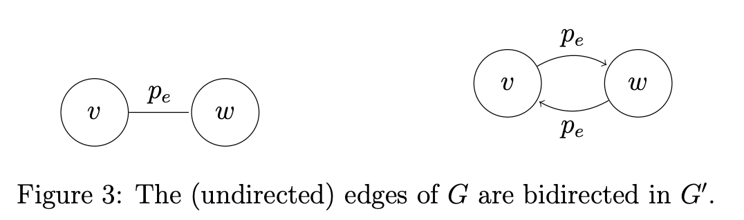
-
missing source and sink? Add them to the new graph $G’$ so that $V’ = V \cup {s,t}$
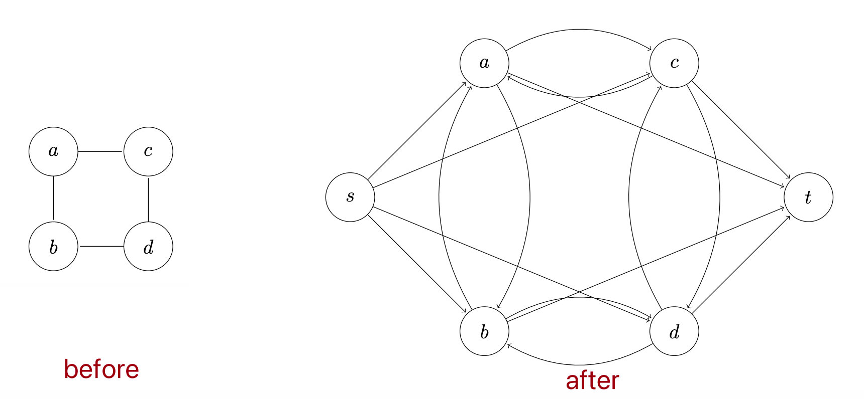
where we can make $s$ the source by adding a directed edge from $s$ to every edge in $V$ but not $t$, and similarlity make $t$ the sink by adding a directed edge from every edge in $V$ but not $s$ to $t$:
-
additional $a_v, b_v$ costs? Since now we have an edge from $s$ to every vertex $v \in V$, we can just assign $a_v$ to the capacity of that edge, and similarly for $b_v$.
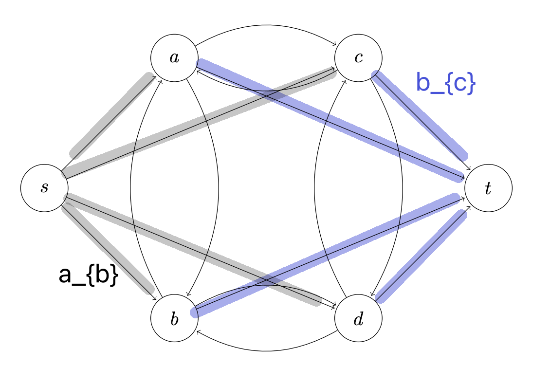
Now, compare the two graphs we get $G$ and $G’$:
-
there is a bijection where every parition $X,Y$ of $V$ will correspond to a cut $A,B$ in $G’$. This is basically because we can just have $A \iff X \cup {s}$ and $B \iff Y \cup {t}$.
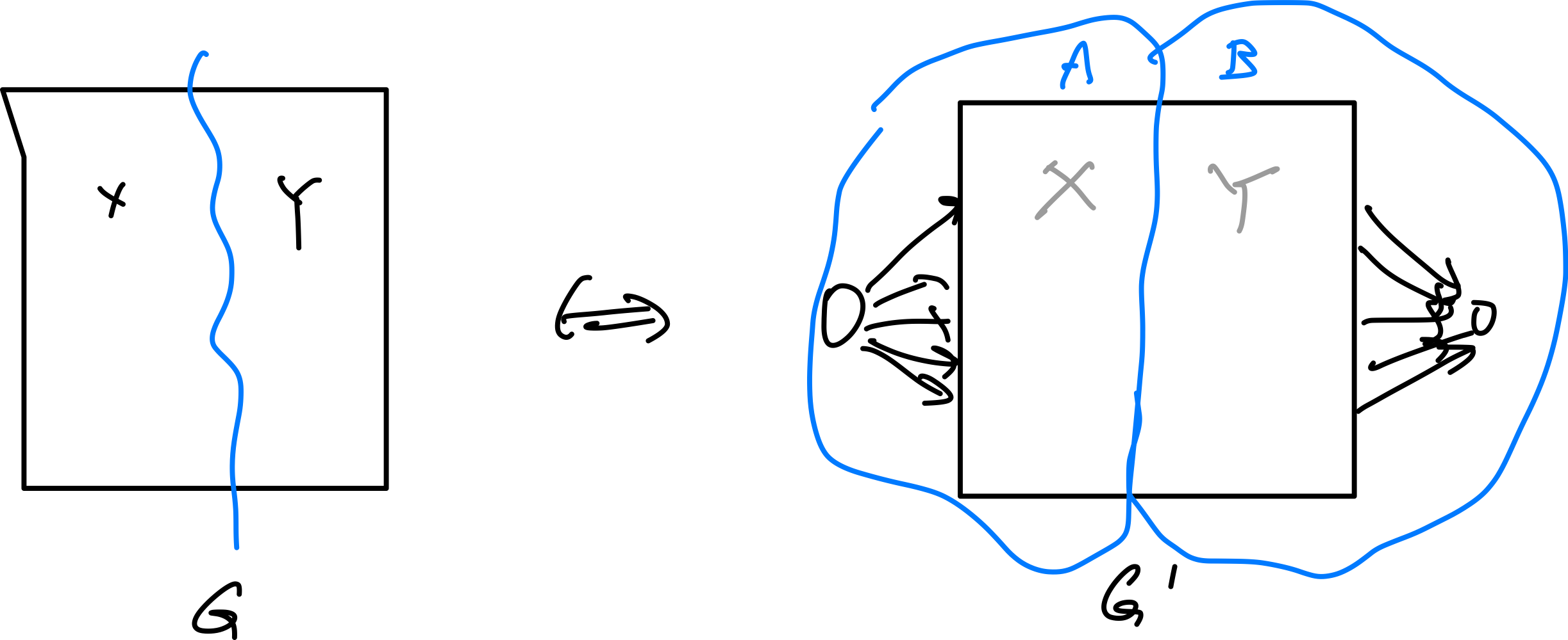
-
then we argue that computing the capacity $\sum_{e =(u,v); u \in A, v \in B} c_e$ of such cut in $G’$ is the same as computing the objective function of $\sum_{v \in X} b_v +\sum_{v \in Y} a_v + \sum_{e \in \delta(X)} p_e$. How?
Consider computing the capacity of the cut $A,B$ in $G’$. You see that the edges that going across $A,B$ would be:
- for every $v \in Y$, we pay $a_v$ for edges $(s,v)$ which crosses the boundary (left to right)
- for every $v \in X$, we pay $b_v$ for edges $(v,t)$ which crosses the boundary (left to right)
- finally we pay $p_e$ for all the edge that starst in $A$ and ends in $B$ (which is exactly $\sum_{e \in \delta(X)} p_e$)
adding all the above up we get exactly $\sum_{v \in X} b_v +\sum_{v \in Y} a_v + \sum_{e \in \delta(X)} p_e$ for $G$.
-
since we can minimize the capacity in $G’$, we can minimze $\sum_{v \in X} b_v +\sum_{v \in Y} a_v + \sum_{e \in \delta(X)} p_e$, which maximizes the original objective function.
-
finally to reconstruct the partition $X,Y$ from the cut $A,B$, we just remove $s$ from $A$ and $t$ from $B$.
Maximum Flow Algorithm
Similar to minimum flow, we start with a flow graph $G=(V,E)$ wth directed edges, a source vertex $s$ and a sink $t$. Each edge $e \in E$ has a capacity $c_e$. The goal is to find a “flow” $f$ that maximizes the total flow from $s$ to $t$.
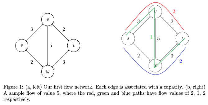
where in the right flow, we made “three streams of water flow”:
- path $s \to v \to t$ with flow 2, because the $v\to t$ bottlenecks at 2
- path $s \to w \to t$ with flow 2, because the $s\to w$ bottlenecks at 2
- path $s \to v \to w \to t$ with flow 1, because the $s \to v$ only has 1 capacity left
But how do we formalize this into a problem (and find an algorithm to solve it)? First, we need to redefine what it means to be a valid flow:
| View 1 | View 2 |
|---|---|
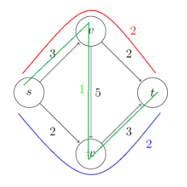 |
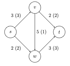 |
and notice that these two are equivalent: specifying a configuation of valid flow is the same as obeying the conservation principle. If each edge is spending $\le$ its full capacity and for each vertex (except for $s,t$) the total outflow equals total inflow, then it is a valid flow. (Note that this understanding is critical to figure out why the algorithm works.)
Therefore, this gives us the formal definition:
Maximum Flow Problem: given a flow graph, assign a flow amount $f_e \ge 0$ to every edge such that:
- for every edge $e \in E$, $f_e \le c_e$ (i.e. you cannot exceed the capacity)
- for every vertex $v \in V \setminus {s,t}$, the total inflow equals total outflow
the goal is to maximize the total flow from $s$ to $t$ = total flow out of $s$ = total flow into $t$.
The intuition of solving this is to first try a intuitive greedy approach, figure out what went wrong, and attempt to fix that (magically reach the correct algorithm in this case).
Naive Greedy Maximum Flow Algorithm
Idea: start with the all-zero flow (i.e. all edges assigned $f_e = 0$) and greedily produce flows with ever-higher value:
- find a viable path $s \overset{P}{\leadsto} t$ in the graph (i.e. can send flow through) using BFS/DFS while checking $f_{e} \le u_e$ does not exceed capacity
- if none exist, then we are done
- if found, find how much we can send through on that path $\Delta = \min_{e \in P} (u_e - f_e)$ where $f_e$ represents the current flow we assigned on that edge
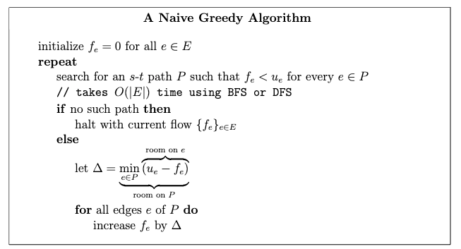
Technically this is already greedy, to make it “greedier” consider step 1 to always pick the path that has highest $\Delta$. Either way, we show that this algorithm is incorrect:
| Greedy Output | Optimal Output |
|---|---|
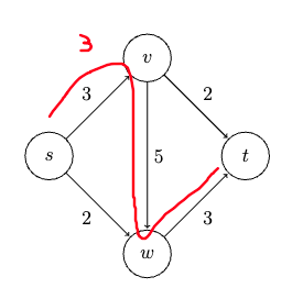 |
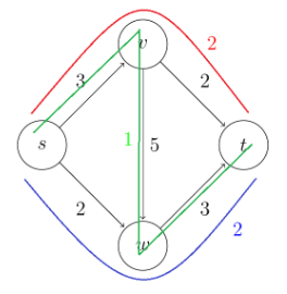 |
where the greedy algorithm can be “unlucky” in that if it picked the zig-zag path in the first iteration, then it has to terminate with flow 3. But the optimal solution is flow 5.
Residual Graph and the Ford-Fulkerson Algorithm
The key idea is to imagine to be able to send flow backward along the edge. How does this work? Essentially it relies on the equivalent view that all we need is conservation of flow at each vertex. For example considering the blue path:
| Sending Flow Backward | Optimal Solution |
|---|---|
 |
 |
Now notice that these are the same! Because we are sending flow in the opposite direction, we can just subtract that from the existing flow we assigned (alike thinking about Kirchoff’s law in circuits). This is the idea of the residual graph:
Residual Graph: given a flow graph $G=(V,E)$ with a flow $f$ assigned to each edge, the residual graph $G_f$ is defined as:
- the same set of vertics
- but with two directed edges for each edge in $G$ an edge $e = (v,w)$ that carries flow $f_e$ spawns into a forward edge of $G_f$ with capacity $u_e - f_e$, and a backward edge with capacity $f_e$.
Visually:
and as a result, any feasible flow in $G$ must still be feasible in $G_f$, because the remaining flow is kept by the forward edge. But since we now also have backward edges, the “search space” for possible flows is now larger. Though how is this useful?
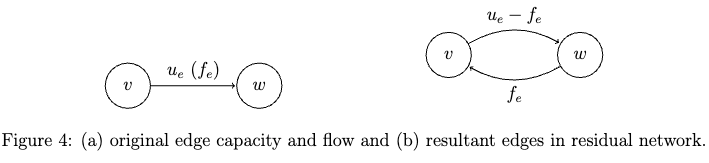
First a concrete example of what a redidual graph looks like:
| Given a flow $f$ graph | Resdiual $G_f$ verbose | Residual $G_f$ simplified |
|---|---|---|
|
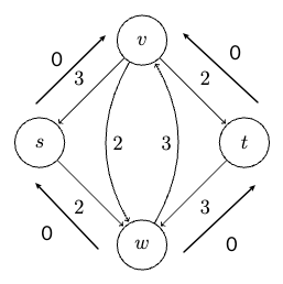 |
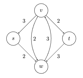 |
where essentially now:
- the forward edge in residual graph means how much flow can you still send out
- the backward edge is how much you can undo, i.e. from the flow you already sent out
We now show that the Ford-Fulkerson algorithm just needs to use that residual graph to be correct:
def ford_fulkerson():
  initialize {f_e} to be all zero
  G_f = residual_graph(G, {f_e})  # a residual graph is defined with a flow
  while True:
    # simple modified DFS/BFS can do this in O(m)
    P = find_path(G_f, s, t)  # find a path in RESIDUAL graph s.t. every edge has positive capacity
    if P is None:
      return {f_e}
    else:
      Delta = min(capacity of e in G_f in that path P)  # find the bottleneck capacity

      # increase the flow from what we found
      for e in P:
        if e is forward edge in G:  # flow in the real graph
          f_e += Delta
        else:
          f_e -= Delta
    G_f = residual_graph(G, {f_e})  # update the residual graph
where the only difference is that now we are searching for path in the residua graph (which has more options). But why it this correct?
Correctness of Ford-Fulkerson Algorithm
The plan is similar to proving Prim’s Algorithm where we show correctness by:
- FF algorithm outputs a viable flow
- There is some property that gives rises to the maximum flow
- FF output satisfies that property
Proof of Claim 1: The intuition is that every iteration of the algorithm we are maintainining the invariance that ${f_e}_{e \in E}$ is a flow. This is essentially because
- we chose $\Delta$ such that no $f_e$ in the real graph $G$ to become negative or exceeds $u_e$
- every edge still preserves “flow in equals flow out”. Why? Consider a vertex $v \in P$ for a $P$ in $G_f$ we picked at the current iteration of the algorithm. Then there is an edge $(x,v)$ and $(v,w)$ with some flow we assigned. Since this flow assigned is in the residual graph:
- if $(x,v)$ corresponded to the forward edge in $G$, vertex $v$ increased incoming flow by $\Delta$. If $(v,w)$ corresponds also to forward edge, then it increased outgoing flow by $\Delta$. Therefore, the net flow in/out $v$ stayed the same.
- if $(x,v)$ corresponded to the forward edge in $G$, vertex $v$ increased incoming flow by $\Delta$. If $(v,w)$ corresponds also to backward edge, then it decreased incoming flow by $\Delta$. Therefore, the net flow in/out $v$ stayed the same.
- … in total four cases, and all of them preserve the flow in/out $v$.
Therefore, if the algorithm halted, the flow ${f_e}_{e \in E}$ is a viable flow. Finally, since every iteration of the algorithm increases the value of the current flow by $\Delta > 0$, and since there is only a finite amount of flow that can come out of $s$ source, the algorithm will terminate eventually.
Proof of Claim 2: Recall that in a directed graph $G$ with a source $s$ and sink $t$, an $s-t$ cut is a partition of $V$ into $A,B$ such that $s \in A$ and $t \in B$. The capacity of the cut is the sum of the capacities of edges crossing from $A$ to $B$. We claim that
Optimality Condition for Max Flow: let $f$ be a valid flow in graph $G$, then:
- $f$ is a maixmum flow
- $\iff$ there is an $s-t$ cut with capacity equal to the value of $f$
- $\iff$ there is no $s \leadsto t$ path with positive capacity in the residual graph $G_f$
where condition 3 is basically when FF algorithm terminates, so if we can prove this then we are done.
(note that condition 3 is quite “strong”, it means all you need to do is to somehow come up with a flow $f$ such that the residual network has no more viable $s \leadsto t$ path.)
First we show that condition (2) implies condition (1)
The intuition is that for ean $s-t$ cut we do, that cost will include all the edge costs that flows out of $A$. Therefore, for any flow configuration $f$, it will consist of path that goes out from $A$ to $B$. Since the maximum/best case scenraio is the flow configuration exhausts all out-flowing capacity, therefore:
\[\text{value of any }f \le \text{capacity of any }s-t \text{ cut}\]To prove this inequality a bit more formally, the value $f$ of any flow can be considered as
\[\text{value of }f = \sum\limits_{e \in \delta^{+}(s)} f_{e} = \sum\limits_{e \in \delta^{+}(s)} f_{e} - \underbrace{\sum\limits_{e \in \delta^{-}(s)} f_{e}}_{\mathrm{zero}}\]since $\delta^{-}(s) = \empty$ as source has no incoming edges. Then, consider any $A,B$ cut in residual graph $G_f$. Since the conservation property hold, all other vertices will have the two terms zero:
\[\text{value of }f = \sum\limits_{v \in A} \left( \sum\limits_{e \in \delta^{+}(v)} f_{e} - \sum\limits_{e \in \delta^{-}(v)} f_{e} \right)\]which is essentially to count every edge’s contribution in $A$. But then that is essentially treating $A$ as a giant “source” vertex, so that:
\[\text{value of }f = \sum\limits_{e \in \delta^{+}(A)} f_{e} - \sum\limits_{e \in \delta^{-}(A)} f_{e}\]Then the rest is obvious: all the flow coming out of $A$ cannot be larger than the capacity $u_e$, and all $f_e$ back into $A$ are non-negative, so:
\[\begin{align*} \text{value of }f &= \sum\limits_{e \in \delta^{+}(A)} f_{e} - \sum\limits_{e \in \delta^{-}(A)} f_{e} \\ &\le \sum\limits_{e \in \delta^{+}(A)} u_e - \sum\limits_{e \in \delta^{-}(A)} 0 \\ &= \sum\limits_{e \in \delta^{+}(A)} u_e \\ \end{align*}\]therefore, visually this inequality means:
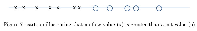
so if value of one of $s-t$ cut overlapped with the cross in the figuer above (condition 2), then that cross has to be the maximum $f$ you can have due to the inequality above $\implies$ condition (1).
Next we show that (1) implies (3)
This is obvious. If by contrapositive that we still find a s-t path in $G_f$, then we can just increase the flow by $\Delta$ and still have a viable flow. But this contradicts the fact that (1) is a maximum flow.
Finally we show (3) implies (2).
If (3) is true (no $s \leadsto t$ path possible in $G_f$), then we can obtain a partition $A$ by just doing a BFS/DFS from $s$ until we get stuck:
\[A = \{ v \in V: \text{ther is an $s \leadsto v$ path in $G_f$} \}\]then the other partition $V-A$ will contain $t$. Additionally, such a cut must look like this:
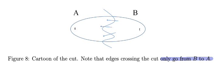
where no (positive) edges would be sticking out of $A$, as otherwise we would have expanded $A$. But what does this cut mean for the original graph $G$?
-
Every edge sticking out of $A$ in $G$ must had assigned $f_e = u_e$ saturated the capacity. If not, then the residual graph $G_f$ would have a positive capacity edge forward edge (representing how much capacity you can still send) sticking out of $A$.
-
Every edge going into $A$ in $G$ must have an assigned $f_{e} = 0$. This corresponds to the residual graph $G_f$ having an edge of $0$ sticking out of $A$ to $B$ (recall that the corresponding backward edge in $G_f$ represents the flow you have already sent out).
Now recall that we had the inequality before, it now becomes equality
\[\begin{align*} \text{value of }f &= \sum\limits_{e \in \delta^{+}(A)} f_{e} - \sum\limits_{e \in \delta^{-}(A)} f_{e} \\ &= \sum\limits_{e \in \delta^{+}(A)} u_e - \sum\limits_{e \in \delta^{-}(A)} 0 \\ &= \sum\limits_{e \in \delta^{+}(A)} u_e \\ &= \text{capcity of }(A, V-A) \end{align*}\]this completes the proof.
Reduction to Min Cut
This now becomes trivial, as you recall this figure
The recall that in the third part of Correctness of Ford-Fulkerson Algorithm proof we said
\[\text{value of }f = \text{capcity of }(A, V-A), \quad \text{for $f$ is a max flow}\]therefore the correspdong $(A, V-A)$ parition must be a minimum cut (based on Figure 7 above, corresponding to an overlap of cross and circle).
Runtime of Ford-Fulkerson Algorithm
So what about the runtime? The worst case is $f$ many iterations, where $f$ is the value of the maximum flow in the graph (because we are increasing the flow by $\Delta$ each time). But note that:
Ford-Fulkerson Algorithm always terminates for networks whose edge capacities are integral (or, equivalently, rational). On the other hand, it might fail to terminate if networks have an edge with an irrational capacity.
However, we can make it polynomial time by using BFS to find an augmentation path, which is called Edmonds-Karp algorithm, which we will not cover here.
Reduction to Bipartite Matching
Bipartite Matching Problem: consdier an undirected bipartite graph $G=(V \cup W \cup E)$ (see image below), with every edge of $E$ having one endpoint in each of $V$ and $W$. That is, no edges internal to $V$ or $W$ are allowed. The feasible solutions are the matchings of the graph, meaning we can only pick $S \subset E$ of edges that share no endpoints. The goal is to pair up as many vertices as possible (using edges of $S$)
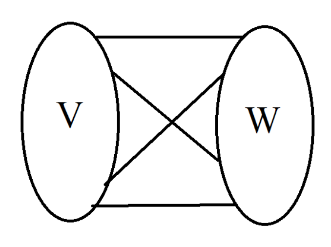
For example, in the following graph, the maximum matching is 1 (pair of vertex):
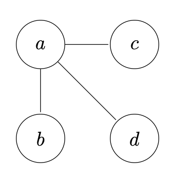
Claim: maximum-cardinality matching reduces in linear time to maximum flow.
The trick is to consider transformation of the bipartite graph $G$ to the following:
where given a bipartite graph $G=(V \cup W \cup E)$, we construct a flow graph $G’$ with:
- add $s$ source with edges to all vertices in $V$ with outgoing capacity exactly 1
- add $t$ sink with edges from all vertices in $W$ with incoming capacity exactly 1
- all other edges from a vertex in $V$ to $W$ can have any capacity greater than 1. Here we use infinity to illustrate this.
Notice that this construction gives any flow in $G’$ to
- use each vertex in $x \in V$ at most once, since there is only one edge that can flow to $x$ and has the bottleneck capacity of 1
- use each vertex in $y \in W$ at most once, since there is only one edge that can flow from $y$ and has the bottleneck capacity of 1
Therefore:
- $\implies$ a bijection between a bipartite matching in $G$ with an integer-valued flow in $G’$
- $\implies$ the bijection also gives the same cost: the size of flow you assigned is th same as the cardinality of the matching
- $\implies$ the maximum flow in $G’$ is the same as the maximum cardinality matching in $G$
Additional Proporties of Flow in Graphs
This section all considers a flow graph $G$ being a directed graph with a source $s$ and sink $t$, and each edge $e \in E$ has a positive, interger capacity $c_e$.
Acyclic Flow: a flow is acyclic if, for every cycle in the flow graph $C \subset G$:
\[C = \{ x_1 \to x_2, x_2 \to x_3, ... , x_n \to x_1 \}\]have at least one edge $e = (x_i, x_{i+1}) \in C$ having a flow of zero $f(e) = 0$. (otherwise we have a cycle flow)
Partitionable Flow: a flow is partitionable if there is a collection of $s,t$ paths flows $P_1, P_2, …, P_{\vert f\vert }$ with paths can be duplicates, $\vert f\vert$ is the value of the flow (i.e. total out of source $s$), and every path just consumes flow of $1$, so that:
\[f(e) = \mathrm{size}( \{ i | e \in P_i \} ), \quad \forall e \in E\]i.e. the flow on an edge $e$ is the number of paths that use that edge.
Then some properties of flow include:
- For every flow, there exists an acyclic flow with the same value.
- every acyclic flow is partitionable
Proof sketch for 1: realize that edges from a source vertex or the sink cannot be involved in any cycle. Therefore, for every cycle in the graph, we can decrement the flow on every edge until one of the edges hit zero. This will result in:
- no change in flow value (since source/sink aren’t affected)
- still a valid flow since for every vertex, the total inflow equals total outflow (since we decremented the same amount into each vertex and out of each vertex)
Proof sketch for 2: We can decompose the flow in the network as follows:
- Identify a path from the source to the sink that carries a positive flow. This can be done by starting at the source and following edges with positive flow until the sink is reached.
- The minimum flow in an edge along this path is the bottleneck of the path. We can consider this as a single unit of flow and subtract this flow value from every edge along this path.
- This process does not violate the flow conservation principle at any node since that path will also be acyclic = i.e. every vertex on the graph is entered and exited exactly once.
- if the original path is cyclic, then this does not work: we may find a cyclic path where a vertex is exited, entered (a cycle), and exited again = net flow in/out is not conserved on that path.
- this will decrease the original flow value of the network by the bottleneck value of the path
- Because the conservation principle holds, the remaining flow is still valid. This means that by definition, if the remaining flow $> 0$, then there must still exists flow paths from the source to the sink with positive flow (i.e. the water is still running).
Repeat the above step until no more paths with positive flow from the source to the sink can be found in the residual network. Each time a path is found, it is distinct and non-overlapping with previously found paths because:
- The flow in an edge cannot be counted more than once since each path uses the minimum flow on its route (the bottleneck), which is then subtracted from the network.
- Once the flow on an edge is reduced to zero, that edge cannot be used in subsequent paths.
Linear Programming
Linear programming is a method to solve optimization problems where the objective function and constraints are linear. It is special in that:
- Linear programming is a remarkable sweet spot between generality and computational efficiency (too general a problem becomes NP-Hard)
- exists many commercial solvers (i.e. algorithm implementations) that can solve those problems within polynomial time
- many problems we have seen in the later part of this course can be formulated as linear programming problems
We will mostly focus on how to reduce problems into a linear programming problem, and not so much on the algorithmic details of solving it.
Ingredients of a Linear Program
So what kind of problems can linear programming solve? The answer is to formulate questions in the following form:
Ingredients of a Linear Program: basically you can specify what variables to solve/be returned, what constraints you have, and what is the objective.
- Decision Variables: the variables you want to solve for, denoted as $x_1, x_2, …, x_{n} \in \R$.
Linear Constraints: you can have as many as you want, but each needs to be in the form of:
\[\sum_{j=1}^n a_j x_j \{* \} b_i\]where $*$ can be $\le, \ge, =$. (Really all you need is $\le$, because to get $\ge$ you can multiply by $-1$ and to get $=$ you can do both $\le$ and $\ge$.)
Linear Objective Function: one objective function to maximize or minimize, in the form of:
\[\max \sum_{j=1}^n c_j x_j\]or the minimum (again, you can just multiply by $-1$ to get the other one).
note that you can specify the $a_j,b_i,c_j$, and the algorithm will solve for the $x_j$.
A starter example is to consider finding the solution to:
\[\max x_1 + x_2\]subject to the following (four) linear constraints:
\[\begin{align*} x_1 \ge 0 \\ x_{2} \ge 0 \\ 2x_1 + x_2 \le 4 \\ x_1 + 2 x_2 \le 1 \end{align*}\]then obviously this fits directly with the linear programming formulation, where $x_1, x_2$ are the decision variables. Visually, this linear problem does:
where the
- dimension of space we are working with is specified by the number of decision variables
- constraints specify the feasible region (the shaded area)
- objective specifies the direction of optimization (the green arrow)
To be more general:
Geometric Interpretation of Linear Programs:
- A linear constraint in $n$ dimensions corresponds to a halfspace in $\R^{n}$. Thus a feasible region is an intersection of halfspaces (i.e. many constraints), the higher-dimensional analog of a polygon.
- The objective function specifies parallel $(n-1)$ dimensional hyperplans, with a direction vector specified by the vector $\vec{c} = [c_1, …, c_n]$. (in the previous example, $\vec{c} = [1,1]$)
- The optimal solution is the point in the feasible region that is furthest in the direction of $\vec{c}$.
- When there is a unique optimal solution, it is vertex (i.e. a corner) of the feasible region.
besides the above, also note that for any given linear programming problem:
- There might be no feasible solutions at all
- optimal objective function value might be unbounded, which the linear programming algorithms should detect if this is the case
- there might be multiple optimal solutions. Whenever the feasible region is bounded, however, there always exists an optimal solution
Example Applications of Linear Programming
Zillions of problems reduce to linear programming. Here we cover a few interesting ones.
Linear Programming for Maximum Flow
The problem of maximum literally translates directly to a linear program (though Ford-Fulkerson algorithm is more efficient).
Proof: in maximum flow we wanted to find a flow for each edge $f_e$, such that the sum of flow is maximum, subjective to conservation constraints. This sounds exactly like linear programming:
- Decision Variables: the flows for each edge ${ f_e }_{e \in E}$
-
Constraints: We needed the conservation contraints, and the capacity constraints
\[\sum\limits_{e \in \delta^{+}(v)} f_e - \sum\limits_{e \in \delta^{-}(v)} f_e = 0, \quad \forall v \in V \setminus \{s,t\}\]which gives $n-2$ constraint equations, where $e \in \delta^{+}(v)$ means edges going out of $v$ and $e \in \delta^{-}(v)$ means edges going into $v$. Then we additionally have for each edge:
\[f_{e} \le u_e\]and finally
\[f_e \ge 0\]So in total this is $n-2+2m$ contraints. Note that these are all linear (each decision variable $f_e$ only appears by itself with some constant)!
- Objective Function: simply:
which you can do by specifing a weight $c_j$ to be one only for edges from the source and zero otherwise.
Linear Programming for Minimum-Cost Flow
Problem: in addition to maximum flow, consider two changes:
- there is a cost $c_e$ associated with each unit of flow spent
the flow is required to be exactly $d$
\[\sum_{e \in \delta^{+}(s)} f_e = d\]so the objective function is to minimize routing over “expensive pipes”:
\[\min \sum_{e \in E} c_e f_e\]
Notice that this can be reduced to the same linear program in the previous section, but with:
- an additional constraint: $\sum_{e \in \delta^{+}(s)} f_e = d$
- objective function changed to $\min \sum_{e \in E} c_e f_e$ (which is linear since $c_e$ are constants)
Linear Programming for Regression
We now consider two less obvious applications of linear programming, to basic problems in machine learning.
Regression: consider inputs of labeled data ${ \vec{p}^{1}, \vec{p}^{2}, …, \vec{p}^{m} }$ consisting of $m$ data points in $\R^{d}$, and their corresponding labels ${ y^{1}, y^{2}, …, y^{m} }$, where $y^{i} \in \R$.
- for example, a dataset of features of $m$ undergraduate students, and $y^{i}$ are their GPAs.
The goal is to find a linear function $h(\vec{z}) = \vec{w} \cdot \vec{z} + b= \sum_{i=1}^{d} w_i z_i + b$ that fits this data as well as possible.
We now show that computing the best line under the definition of minimizing absolute error can be formulated as a linear program (for the more common one, mean squared error, check the ML notes).
First recall that for a $d$-dimensional space, a linear function $h : \R^{d} \to \R$ has the form:
\[h(\vec{z}) = \vec{w} \cdot \vec{z} + b = \sum_{i=1}^{d} w_i z_i + b\]where the coefficients $w_i$’s and $b$ are unknown. The absolute error for one data point is defined as:
\[E_i ( \vec{w} ,b) = \left| \underbrace{\left( \sum\limits_{j=1}^{d} w_j p_j^{i} +b\right)}_{\text{prediction}} - y^{i} \right|\]and so the total loss over the entire dataset is:
\[\min_{\vec{w} ,b} \sum\limits_{i=1}^{m} E_i(\vec{w} ,b)\]note that up to this point, this problem had:
- $d+1$ decision variables: $\vec{w} ,b$
- no constraints for the weights and bias
- a nonlinear objective function (because it used absolute value)
So how is this linear programmable? The trick is we can convert the absolute value in objective function to become constraints. Consider introducing $m$ new decision variables $e_1, e_2, … , e_m$ which would represent $E_i ( \vec{w} ,b)$. We make it look like it can choose $e_i$, but in fact not because we know:
\[| x| = \max \{ x, -x \}\]so we can get inequalities to represent absolute values:
\[e_{i} \ge \left( \sum\limits_{j=1}^{d} w_j p_j^{i} +b \right) - y^{i} \\ e_{i} \ge - \left( \sum\limits_{j=1}^{d} w_j p_j^{i} +b \right) + y^{i}\]and the objective function is:
\[\min \sum\limits_{i=1}^{m} e_i\]so that now we consider
- $d+1+m$ decision variables: $\vec{w} ,b, e_1, e_2, … , e_m$
- $2m$ constraints for the weights and bias
- a linear objective function where obtaining the best $e_i$’s becomes obtaining the best absolute error (think about obtaining a better $e_i$ subject to this contraint is the same as obtaining $\vec{w},b$ with a lower loss )
note that the $e_i$ under the hood aren't ''free'' variables:
- After the program found out about $w_j$ and $b$, the $e_i$’s are determined by picking to be as close as possible to the inequality (i.e. represents the absolute error) because of the objective function being a minimizer
- then, the objective function also correctly represents the total absolute error
Linear Programming for Linear Classifier
Linear Classifier: consider inputs of binary classification, where you get $m$ positive data points $\vec{p}^{1}, …, \vec{p}^{m} \in \R^{d}$ and $m’$ negative data points $\vec{q}^{1}, …, \vec{q}^{m’} \in \R^{d}$.
The goal is to compute a linear function $h(\vec{z}) = \vec{w} \cdot \vec{z} + b= \sum_{i=1}^{d} w_i z_i + b$ that separates the positive and negative data points as well as possible. In other words:
\[h(\vec{p}^{i}) > 0, \quad \forall i \in [m] \\\]and for negative points:
\[h(\vec{p}^{i}) < 0, \quad \forall i \in [m'] \\\]
Visually, it looks likes:
Assuming there exists such a classifier, the problem almost looks exactly like a linear program, except that we have strict inequalities here. Again, the simple trick of adding an extra decision variable solves the problem.
To encode this strict inequality, we introduce a new decision variable $\delta$ representing the margin by which the nearest data point is on the correct side of the decision boundary. Then we have a new constraint with inequality:
\[\sum\limits_{j=1}^{d} w_j p_j^{i} +b \ge \delta, \quad \forall i \in [m] \\ \sum\limits_{j=1}^{d} w_j q_j^{i} +b \le -\delta, \quad \forall i \in [m']\]with the objective of maximzing the margin $\delta$:
\[\max \delta\]so that we have a linear program with:
- $d+2$ decision variables: $\vec{w} ,b, \delta$
- $m + m’$ constraints for the weights and bias
- a linear objective function
(note that this looks awfully like SVM)
However, what if the points aren’t perfectly separable? In SVM we had slack varittlables, but here we can consider another extension: allow for errors, but penalize them.
More specifically, let’s say that in a perfect world, we would like a linear function $h$ such that:
\[h(\vec{p}^{i}) > 1, \quad \forall i \in [m] \\\]and
\[h(\vec{q}^{i}) < -1, \quad \forall i \in [m'] \\\]where the constant $1$ is a bit arbitrary here. Though the goal is to consider a hinge loss such that it penalizes on incorrect classifications, but gives zero loss as long as you have a correct classification with a margin of at least $1$:
\[\mathrm{loss} = \begin{cases} \max \{1 - h(\vec{p}^{i}), 0 \}, \quad \text{for positive points}\\ \max \{1 + h(\vec{q}^{i}), 0 \}, \quad \text{for negative points} \end{cases}\]so then our task is to find a linear function that minimizes total hinge loss. While hinge loss looks non-linear, it really is just the maximum of two linear functions. We claim that this can be formulated as a linear program with constraints:
\[\begin{align*} e_i &\ge 1 - \left( \sum\limits_{j=1}^{d} w_{j} p_j^{i} +b \right), \quad \text{for every positive point $\vec{p}^i$ }\\ e_i &\ge 1 + \left( \sum\limits_{j=1}^{d} w_{j} q_j^{i} +b \right), \quad \text{for every negative point $\vec{q}^i$ }\\ e_i &\ge 0, \quad \text{for every point} \end{align*}\]which is basically the hinge-loss, and then the objective is:
\[\min \sum\limits_{i=1}^{m} e_i\]so again, we introduced $m$ new decision variables $e_i$ which aren't real ''free'' variables:
- After the program found out about $w_j$ and $b$, the $e_i$’s under the hood are determined by picking to be as close as possible to the inequality (i.e. represents the hinge loss) because of the objective function being a minimizer
- then, the objective function also correctly represents the total hinge lossa