NP-Hard Problems

Beyond the collection of efficient algorithms we have talked about? In the first part of the notes, we have seen problems such as sorting, graph search, shortest path, MST, etc being solved in almost linear time. Here, we essentially discuss the class of problems for which NO fast algorithms are KNOWN (notice the distinction between “no fast algorithms exist” and “no fast algorithms are known”).

The Traveling Salesman Problem

By definition, this looks very alike MST:

Traveling Salesman Problem Definition: given a complete undirected graph $G=(V,E)$ and a real-valued cost $c_e$ for each edge $e\in E$, find a minimum-cost tour that visits each vertex exactly once.

difference from MST: MST is a spanning tree while TSP is a tour.

technically MST had only needed “connected” graph, which is actually more general (as you can mimic non-complete graphs by having some edges cost $\infty$)

How many distinct tours are there? Since each tour is a cycle, we have $n! / (2n)$ because for each vertex, it is repeated twice (once as start, once as end).

Despite significant effort, until today (2023) there is no known fast algorithm for the TSP.

Conjecture: maybe no fast algorithm exists for TSP.

But how do we even attempt to “prove” this? (Spoiler: we kind of don’t. We just try to show TSP is NP-hard $\implies$ solving it efficiently would prove $\mathcal{P} = \mathcal{NP}$, and until today no-one has done it.)

Introduction to P and NP

Polynomial-Time Algorithms

So what does it mean to be $\mathcal{P}$?

Polynomial-Time Solvable Problems A problem is in $\mathcal{P}$ if there is a polynomial-time algorithm to solve it.

polynomial-time algorithm: one that correctly solves the problem with worst-case running time $O(n^k)$ for some constant $k$.

here $n$ denotes the input size, which you can image as “the number of bits needed to represent the entire input” for a generic problem.

NP-hard Problems

Going back to our original problem: the goal is to gather evidences to show that “there exists no polynomial-time algorithm for TSP”. Just to be clear, no one has proven this yet, but we have some evidence to support this conjecture: to show that TSP is relatively speaking, hard.

Strong Evidence of A Problem being Hard: A polynomial-time algorithm for the TSP would solve thousands of problems (i.e. by reduction), that have resisted the efforts of tens (if not hundreds) of thousands of brilliant minds over many decades.

basically TSP must be “at least as hard as” any of those other problems.

More formally, here comes the notion of NP-hardness.

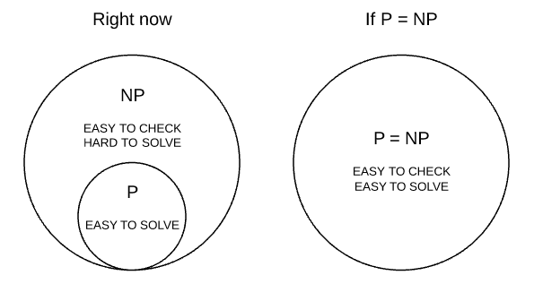
Complexity Class $\mathcal{NP}$: a problem is in $\mathcal{NP}$ if

for every instance of the problem, every candidate solution can be described (e.g. in bits) by using, bounded above, a polynomial function of the input size.

for any of the candidate solutions, we can verify in polynomial time whether it is indeed a valid solution.

Notice that by this definition, almost all the search problems that you’ve seen qualify for $\mathcal{\mathcal{NP}}$. But additionally, let every candidate solution be described in $O(n^{d})$ bits, for an instance of the problem having input size $n$. Then, an exhaustive search algorithm over all solutions is:

\[O(2^{O(n^{d})}) \times O(n^{k}) = O(2^{O(n^{d})})\]

where:

since every solution can be described/encoded in $O(n^{d})$ bits, there are $2^{O(n^{d})}$ possible solutions.
the exhaustive search would basically loop over all possible solutions, and for each solution, it would take $O(n^{k})$ time to verify whether it is indeed a valid solution.
this therefore is exponential runtime (but of course, many problems have smart algorithms to solve them)

NP-hard Problems: a problem is $\mathcal{NP}\text{-}\mathcal{hard}$ if every problem in $\mathcal{NP}$ can be reduced to it in polynomial time.

recall if A reduces to B, then it means we can use B as a black-box to solve A.

so the consequence is that if you can solve one $\mathcal{NP}\text{-}\mathcal{hard}$ problem in polynomial time, you can solve all $\mathcal{NP}$ problems in polynomial time.

then $\mathcal{P} = \mathcal{NP}$

notice that a problem can be $\mathcal{NP}\text{-}\mathcal{hard}$ without being in $\mathcal{NP}$ (see figure at the end of this section)

We will see a bit later that TSP is $\mathcal{NP}\text{-}\mathcal{hard}$ being a strong evidence that we think there exists no polynomial-time algorithm for TSP (basically by reducing the 3-SAT problem to it, and somebody has already done the hardest work showing that 3-SAT is $\mathcal{NP}\text{-}\mathcal{hard}$)!

But visually this means that there is a bunch of $\mathcal{NP}$ problems $A_i$’s such that:

In addition, since no-one so far has solved in polynomial time any $\mathcal{NP}\text{-}\mathcal{hard}$ problem, we have:

Conjecture: $\mathcal{P} \neq \mathcal{NP}$. Motivation why it may be true?

empirical: all you need is one polynomial time algorithm for one $\mathcal{NP}\text{-}\mathcal{hard}$ problem to prove $\mathcal{P} = \mathcal{NP}$, but no one has found it yet.

philosophical: if $\mathcal{P} \neq \mathcal{NP}$, then it means “solving a problem is as hard as checking a solution of a problem”. Then life is too easy.

mathematical: as of today, absent of evidence.

A “surprising” example of $\mathcal{NP}$ problem: Knapsack:

recall that there is an $O(nC)$-time dynamic programming algorithm for the problem
but this is NOT polynomial in the size of input. this is a polynomial-time algorithm in the special case in which $C$ is bounded by a polynomial function of $n$.
think of the number of keystrokes to type $C=10$, which is $2$, to $C=100$, which is $3$. The input size increased by $1.5$, but runtime increased by a factor of $10$.

Finally, a more complete picture of P, NP, and NP-hard:

Simple Reductions for NP-Hardness

Recall that we have used reductions before. For instance, to compute the Image Segmentation problem we used a minimum s-t cut algorithm as a black-box (i.e. Image segmentation reduces to minimum s-t cut):

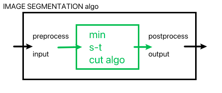
where we:

assumed that minimum s-t cut is polynomial-time solvable (it is)
created the image segmentation problem by preprocessing the input (convert to flow graph) and postprocessing the output (convert back)

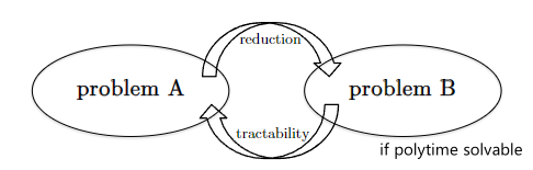
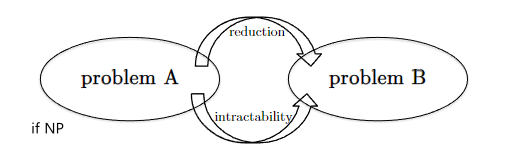
Reductions will also be used here, but for the purpose of spreading intractibiliy or tractibiliy (i.e. polynomial-time solvability) of a problem.

Tractibility	Intractibility

so that more formally:

Reductions Spread Tractability: if $A$ reduces to $B$ and $B$ is solvable in polynomial time, then $A$ is solvable in polynomial time.

Reductions Spread Intractability: if $A$ reduces to $B$ and $A$ is not solvable in polynomial time, then $B$ is not solvable in polynomial time.

think of it as a contrapositive of the previous statement

We have seen many nice examples of the first part: “spreading tractability”, in addition to the image segmentation problem:

Finding the median of an array of integers reduces to the problem of sorting the array
The all-pairs shortest path problem reduces to the single-source shortest path problem (iterating over all vertices is still polynomial time)

But the latter part: “spreading intractability” is like the dark-side of the force, where we use in this case to show many problems are $\mathcal{NP}\text{-}\mathcal{hard}$.

if we know a problem $A$ is $\mathcal{NP}\text{-}\mathcal{hard}$, and we can reduce $A$ to $B$, then $B$ is also $\mathcal{NP}\text{-}\mathcal{hard}$. Why?
because if $B$ is solvable in polynomial time (the green box in the image segmentation example), then $A$ is also solvable in polynomial time.
This would imply all other $\mathcal{NP}$ problems are solvable in polynomial time (since $A$ is $\mathcal{NP}\text{-}\mathcal{hard}$). Then $\mathcal{P}=\mathcal{NP}$!

Some examples of $\mathcal{NP}\text{-}\mathcal{hard}$ problems?

This also highlights a template for proving if a problem is $\mathcal{NP}\text{-}\mathcal{hard}$:

Proving $\mathcal{NP}\text{-}\mathcal{hard}$: to prove a problem $B$ is $\mathcal{NP}\text{-}\mathcal{hard}$, we can:

find/choose an existing $\mathcal{NP}\text{-}\mathcal{hard}$ problem $A$.

Prove that $A$ reduce to $B$ in polynomial time. (i.e. can use $B$ to solve $A$)

NP-Hardness of Cycle-Free Shortest Paths

Here we discuss an example of known $\mathcal{NP}\text{-}\mathcal{hard}$ problems, and how we can use reduction to show that another problem we discussed in the first part of the notes is also $\mathcal{NP}\text{-}\mathcal{hard}$.

Recall that we had this problem:

Cycle-Free Shortest Path (CFSP): given a directed graph $G=(V,E)$ with real-valued edge costs $c_{e} \in \R$ and a source vertex $s$, find a shortest cycle-free path from $s$ to every other vertex in $G$. If there is no $s-v$ path for some $v$, report $+\infty$ for them.

why did we want cycle free? The problem is that if we had negative cycles, then the shortest path would be $-\infty$

in the first part of the notes, we have seen Bellman-Ford algorithm which find shortest path and “detect negative cycles” in $O(mn)$ time, i.e. break when there is a negative cycle.

We want to prove that this version of the problem is $\mathcal{NP}\text{-}\mathcal{hard}$

Directed Hamiltonian Path (DHP): given a directed graph $G=(V,E)$, output “yes” if there exists a directed path that visits each vertex exactly once, and “no” otherwise.

This is a famous $\mathcal{NP}\text{-}\mathcal{hard}$ problem in computer science.

Now we want to show that DHP reduces to CFSP. Therefore since DHP is $\mathcal{NP}\text{-}\mathcal{hard}$, CFSP is also $\mathcal{NP}\text{-}\mathcal{hard}$.

Proof: The key question to think is: how do we use a subroutine for the cycle-free shortest path problem to solve the directed Hamiltonian path problem? In the former it will find shortest cycle-free path, whereas the latter needs a path that visits each vertex exactly once. Some key insights would be:

trick the CFSP into thinking that long paths (like an s-t Hamiltonian path) are actually short
to achieve this, we can assign $c_{e} = -1$ for every edge $e$ in the graph

Therefore, consider the following reduction for DHP:

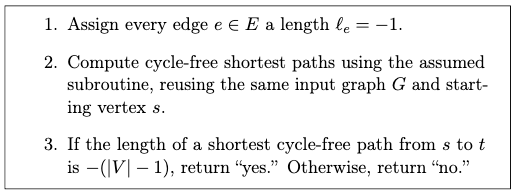
Why can this algorithm (embedded with CFSP subroutine) solve DHP, i.e. is correct? To show this, we need to prove that this algorithm will output “yes” if and only if there is a Hamiltonian path in the graph. Notice that:

in the constructed cycle-free shortest paths instance, the minimum length of a cycle-free s-t path equals $-1$ times the maximum number of hops
given a $s,t$, how do we get maximum hops in this case? Visit as many vertices as possible.
therefore, a cycle-free shortest path uses $\vert V\vert - 1$ hops at most, in which case it is a Hamiltonian path.

Hence, we just need to check if the shortest path from $s$ to $t$ is of length $-(\vert V\vert - 1)$. This would correctly solve DHP problem.

Rookie Mistakes and Acceptable Inaccuracies

Here are a few common misunderstandings about the notion of $\mathcal{NP}\text{-}\mathcal{hard}$.

Rookie Mistakes: (plain wrong)

thinking $\mathcal{NP}$ stands for “not polynomial time solvable”
using $\mathcal{NP}$ and $\mathcal{NP}\text{-}\mathcal{hard}$ interchangeably.
- this is because in $\mathcal{NP}$ is actually a “good thing”. as it tells us a problem can be verified in polynomial time (but says nothing about how quickly we can solve it)

Acceptable Inaccuracies:

Assuming $\mathcal{P} \neq \mathcal{NP}$ is true
Using the terms $\mathcal{NP}\text{-}\mathcal{hard}$ and $\mathcal{NP}\text{-}\mathcal{complete}$ interchangeably.
- $\mathcal{NP}\text{-}\mathcal{complete}$ is a subset of $\mathcal{NP}\text{-}\mathcal{hard}$, and the practical implications is the same as $\mathcal{NP}\text{-}\mathcal{hard}$.
- assuming $\mathcal{P} \neq \mathcal{NP}$ is true, then both $\mathcal{NP}\text{-}\mathcal{hard}$ and $\mathcal{NP}\text{-}\mathcal{complete}$ are not solvable in polynomial time.
Conflating $\mathcal{NP}\text{-}\mathcal{hard}$ with requiring exponential time in the worst case

Compromising on Correctness: Efficient Inexact Algorithms

At the end of the day, you still have to come up with some algorithms to solve NP-hard problems. Because it’s NP-hard, you (probably) are confident that your algorithm can only achieve two out of the three properties:

fully general
always correct
fast

In fact, we have already seen algorithms that compromises on generality over this course. For instance:

Dijkstra’s algorithm assumes non-negative edge costs
Bellman-Ford algorithm assumes graphs without negative cycles
Maximum Weighted Independent Set assumes path graphs
a polytime Knapsack algorithm assumes $C$ is bounded by a polynomial function of $O(n^{k})$

Therefore, instead of compromising on generality, in this section we will discuss algorithms that compromise on correctness, i.e. they are NOT always correct, but often we can quantify an upper-bound of how much error they can make.

Note: this makes greedy algorithms particularly suitable for this purpose, as they are often fast and general, but not always correct.

Makespan Minimization

This is another scheduling problem like the one we have seen in the first part of the notes, but we have a few changes:

Makespan Minimization: given $n$ jobs with processing times $l_{i}$, and $m$ machines, find an assignment of jobs to machines that minimizes the makespan, i.e. the maximum completion time of all jobs.

basically a “multi-processing” version of the scheduling problem we have seen before

goal is to minimize the “latest” finishing job

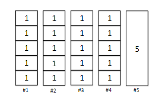
For example, consider four jobs with processing time $l_1=2, l_2=2, l_3=1, l_4=3$, and two schedules:

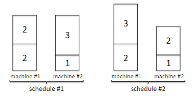
the first one will have makespan $4$, and the second one will have makespan $5$ due to the jobs on the first machine. So intuitively, we an ideal schedule would have a perfectly balanced-load on every machine. But unfortunately:

Makespan Minimization is NP-Hard: there is (currently) no polynomial-time algorithm for makespan minimization

So what kind of algorithm can solve this in a general case, is fast, but may not always give us the best answer?

Graham’s Algorithm

The intuition is that our goal is create a balanced load on every machine, so that the makespan is minimized. Therefore, we can just have a greedy algorithm that iteratively assigns the next job to the machine with the smallest load.

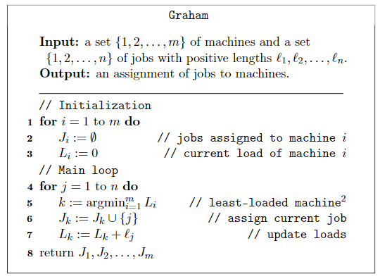
where for a fast argmin implementation, we can use a min-heap to keep track of the smallest load machine. But why this algorithm specifically? It turns out that this is not only fast (with min-heap) giving $O(n \log m)$, but also guarantees a rather good error bound.

Graham’s Algorithm Error Bound

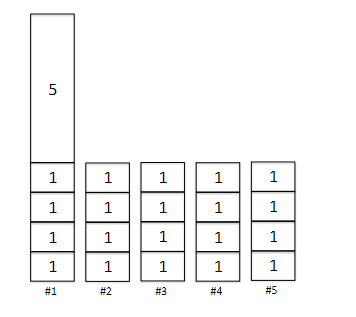
First, let’s demonstrate one example where Graham’s algorithm is not optimal. Consider having 20 jobs with processing time $l_i = 1$ for all $i$, and one last job with processing time $l_{21} = 5$. Suppose we have $m=5$ machines. Then:

Graham’s Algorithm	Optimal Solution

where Graham would output a makespan of $9$, whereas the optimal solution would be $5$. This is quite bad, but can it be worse? The answer is actually no, that this is as bad as it can get.

Graham’s Algorithm Error Bound: Graham’s algorithm is guaranteed to produce a schedule with makespan $\le 2$ times the optimal makespan.

with some algorithmic modifications, we can actually get the error bound to $4/3$ times the optimal makespan.

technically, it is $2 - 1/m$, where $m$ is the number of machines

technically, it is $\le 2$ any possible optimal makespan

in practice, Graham’s (often) does much better than this error bound.

But how can we even go about proving it if we don’t even know what the optimal solution is (as it is NP-hard)? The key idea is to compare with the lower bound of what any optimal solution can achieve, i.e., a perfect load balance.

Proof: First, we need to consider the lower bound of this problem. Let the minimum possible makespan schedule be $M^{*}$. Then:

Lower Bound #1: every job needs to be processed, so the best completion time must be at least as big than any of the processing time:
\[M \ge l_{j}\quad \forall j \in \{1, \ldots, n\}\]
or alternatively $M^{*} \ge \max l_j$.
Lower Bound #2: as the best case scenario is to have a perfectly balanced load (why? If not, one machine will have a larger load and another smaller. But since the objective is the maximum makespan, it is strictly worse):
\[M^{*} \ge \frac{1}{m} \sum_{j=1}^{n} l_{j}\]

Now we consider the lower bound of Graham’s algorithm. Let $M$ be the makespan of the schedule produced by Graham’s algorithm. Consider the “worst” machine that contributed to this load $M$, i.e. the machine with largest load $L_i$ such that $L_{i} = M$. Rewind the algorithm to the point where that machine was assigned its last job $j$, and let $\hat{L}_i$ denote that machine’s load at that point. So that obviously:

\[M = L_{i} = \hat{L}_{i} + l_{j}\]

But how big was $\hat{L}_{i}$? By the greedy criterion of the algorithm, it must have looked like this (if that machine is #1):

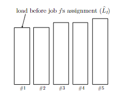
i.e. it must be the lightest loaded before $j$ is assigned. How light can that be?:

\[\hat{L}_{i} \le \frac{1}{m} \sum_{k=1}^{j-1} l_{k}\]

since the lightest load you can get at that point in time is a perfectly balanced load. Now since the comparison we need to make is:

\[M = \hat{L}_i + l_{j} \le l_{j} + \frac{1}{m} \sum_{k=1}^{j-1} l_{k} \le \text{something }M^{*}\]

we consider the following “tricks”:

transform the above expression:
\[M \le l_{j} + \frac{1}{m} \sum_{k=1}^{j-1} l_{k} \le l_{j} + \frac{1}{m} \sum_{k \neq j} l_{k}\]
where we basically added a bunch of terms ($l_{j+1} / m, l_{j+2} / m, …$ ) so that RHS is of course larger or equal to LHS
the second term above is almost comparable with $M^{*}$, so we do some minor arithmetic operations:
\[l_{j} + \frac{1}{m} \sum_{k \neq j} l_{k} = l_{j} - \frac{l_j}{m} + \frac{1}{m} \sum\limits_{k=1}^{n}l_{k} = \left( 1- \frac{1}{m} \right) l_{j} + \frac{1}{m} \sum\limits_{k=1}^{n}l_{k}\]

Now we can use the lower bound we found above

\[M \le \left( 1- \frac{1}{m} \right) l_{j} + \frac{1}{m} \sum\limits_{k=1}^{n}l_{k} \le \left( 2 - \frac{1}{m} \right) M^{*}\]

because using lower bound #1 we know $\left( 1- \frac{1}{m} \right) l_{j} \le \left( 1- \frac{1}{m} \right) M^{}$ and lower bound #2 tells us $\frac{1}{m} \sum\limits_{k=1}^{n}l_{k} \le M^{}$. This completes the proof.

Longest Processing Time First

Here we discuss a modification of Graham’s algorithm that can achieve a better error bound of $4/3$ times the optimal makespan. The observation is that:

in the contrieved example where we showed Graham’s algorithm is not optimal (given 20 jobs with processing time $l_i = 1$ for all $i$ …), if only the algorithm considered the longest processing time job first, then it would have been optimal.
in the error bound proof, we see that it advocates for making the last job assigned to the least loaded machine as small as possible.

This gives the longest processing time first algorithm, which saves those small jobs for the end:

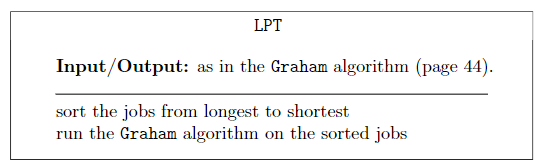
again, this algorithm is not always correct, but it is guaranteed to produce a schedule with makespan $\le 3/2$ times the optimal makespan. How?

Proof: similar to the original Graham algorithm, we start with some lower bounds. Consider we have sorted the jobs from longest to shortest, so that the $j$-th job is longer than the $j+1$-th job.

Modified Lower bound #1: if $M^{}$ denotes the minimum possible makespan, and say we have scheduled the first $m$ jobs (i.e. one for each machine). Let $j$ be *any job after the first $m$ jobs. Then:
\[M^{*} \ge 2l_j\]
which is evident by the pigeon-hole principle: the new job $j$ means we have now ay least $m+1$ jobs to schedule $\implies$ at least one machine had two jobs on it $\implies$ that machine has at least twice the time of $l_j$ since $l_j$ is the shortest amongst those $m+1$ jobs, by construction.

Now, the trick to prove this $3 / 2$ bound is to realize that we can improve the final inequality in the previous proof by having $\left( 1- \frac{1}{m} \right) l_{j} \le \left( 1- \frac{1}{m} \right) (M^{*} / 2)$! Why?

in the same analysis as before, we consider $M$ with the “worst machine” that just got assigned the final job $j$.
there needs to be at least one job assigned to that machine prior to $j$ (otherwise it means there are in total $\le m$ jobs to assign $\implies$ Graham will return the optimal schedule with one job per machine)
this means that job $j$ is after the sorted first $m$ jobs, hence the inequality in modified lower bound applies.

Plugging this in our previous last step:

\[M \le \left( 1- \frac{1}{m} \right) l_{j} + \frac{1}{m} \sum\limits_{k=1}^{n}l_{k} \le \left( 1 - \frac{1}{m} \right) \frac{M^{*}}{2} + M^{*} = \left( \frac{3}{2} - \frac{1}{2m} \right) M^{*}\]

which has a better error bound as the original Graham.

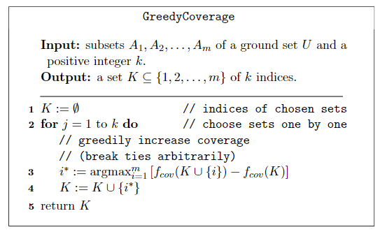
Maximum Coverage Problem

Maximum Coverage Problem: given a collection of subsets $A_1, …, A_{m} \subseteq U$ and a universal ground set $U$, and a number $k$, pick $k$ subsets that reaches the most coverage, i.e. the most number of elements in $U$.

e.g. $A_i$ could represent the programming languages candidate $i$ is familiar with, and $U$ is the set of all programming languages in the world

e.g. the goal is to assemble $k$ candidates such that they cover the most number of programming languages in the world

a bit more formally, pick a choice $K$:
\[K \subseteq \{1, ..., m\}, \quad |K| = k\]
such that $f_{\mathrm{cov}}(K)$ is maximized:
\[f_{\mathrm{cov}}(K) = \left|\bigcup_{i \in K} A_{i}\right|\]

Again, this problem is NP-hard, so we want to come up with an algorithm that is almost always correct. Consider the case when $k=1$: just pick $A_i$ with the largest size. But what about $k=2$? So the intuition is to maybe pick the second subset that increases coverage the most:

This looks good, but when does it break? What is its error bound?

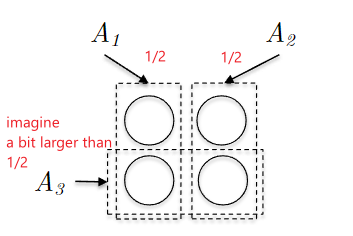
Consider the following example of three subsets with a budget $k=2$:

Input	Greedy Output

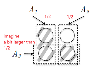where you can achieve all elements by picking $A_1, A_2$. But if $A_3$ is a bit larger than $1 / 2$, then the algorithm would pick $A_3$ and you are immediately screwed: you would only cover about 75% of the elements. Similarly, consider this with budget $k=3$:

Input	Greedy Output

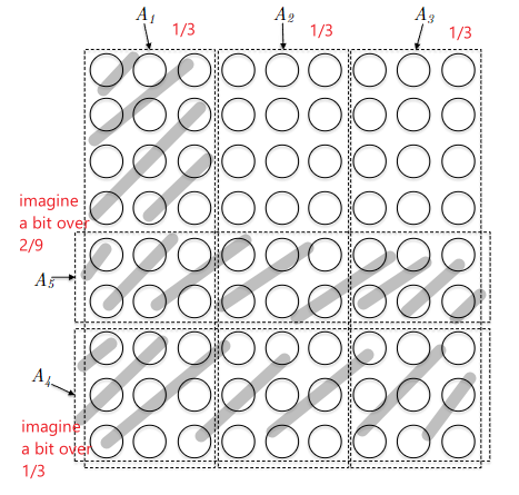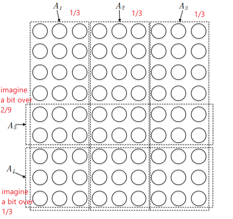
where again, we can trick the greedy algorithm to pick $A_5$ first. Then, this would decrease the contribution of picking $A_1, A_2, A_3$ as they would only roughly contribute $(1 / 3)(2 / 3) = 2 / 9$ portions. Therefore, we can then trick the algorithm to pick $A_4$. Finally, choosing either one of $A_1, A_2, A_3$ would only result in $1 - 2 \times (1 / 3) (4 / 9) = 19 /27 \approx 70\%$ of the total size. But obviously the optimal solution would be to pick $A_1, A_2, A_3$.

Interestingly, before we go into the error bound, we already observe that (if you extend this example to arbitrary $k$):

Bad Examples of GreedyCoverage: for every positive interger $k$, we can come up with an instance such that:

there exists $k$ subsets that reaches $100\%$ coverage

the greedy algorithm picks $k$ subsets might only cover $1 - (1 - 1/k)^{k}$ fraction of the elements.

But since by definition:
\[e = \lim _{n \rightarrow \infty}\left(1+\frac{1}{n}\right)^{n}\]
this is approximately, as $k \to \infty$:
\[\lim _{k \rightarrow \infty} 1 - \left(1 - \frac{1}{k}\right)^{k} \approx 1 - \frac{1}{e} \approx 63\%\]

So in those particular constructions, GreedyCoverage may cover only upto $63\%$ of the elements. But what about the general case? Is this generic enough?

GreedyCoverage Error Bound

It turns out this expression is general for GreedyCoverage, and in fact, it was proven (in other ways) that the number $1 - \frac{1}{e}$ is intrinsic to the maximum coverage problem.

GreedyCoverage Error Bound: the coverage of the greedy algorithm is guaranteed to cover at least $1 - (1 - \frac{1}{k})^{k}$ fraction of the maximum-possible coverage (i.e.. worst-case scenario) for any instance of the problem.

note that guaranteeing to cover $100\%$ would, of course, become an algorithm that is always correct.

To prove this, we need to consider some key lemmas:

Lemma 20.8: consider pausing the algorithm when it has picked $j$ subsets, and let $C_j$ denote the coverage achieved at that point. For each such $j = {1,2, …, k}$, the $j$-th subset we just picked must cover at least $\frac{1}{k}(C^{*} - C_{j-1})$ new elements so that:
\[C_j - C_{j-1} \ge \frac{1}{k}(C^{*} - C_{j-1})\]
where $C^{*}$ is the maximum possible coverage with $k$ subsets.

Proof: let $K_{j-1}$ denote the indices of the $j-1$ subsets picked so far, and $C_{j-1}$ its coverage. Any potential $\hat{K}$ (may or may not be optimal) that contains $k$ indices, and $W$ be the set of elements covered by $\hat{K}$ but not by $K_{j-1}$:

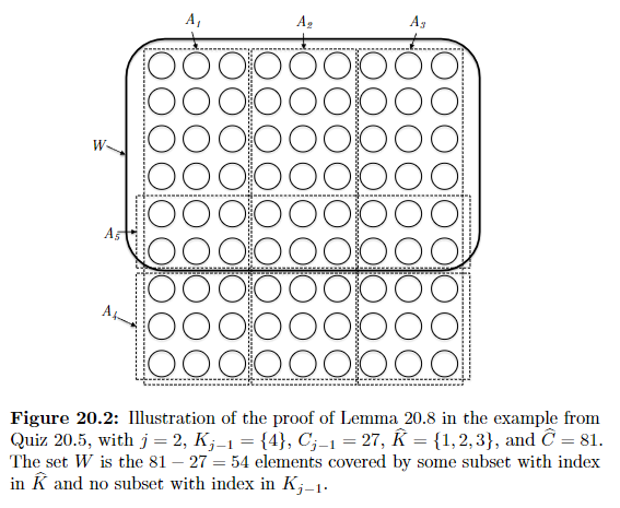
where in the above example, basically $K_{j-1} = {4,5}$ and the alterative $\hat{K}=K^{*}$. Then this means:

\[\sum\limits_{i \in \hat{K}} \left[ \underbrace{f_{\mathrm{cov}}(K_{j-1} \cup \{i\} - C_{j-1})}_{\text{coverage increase by adding $A_i$ into our collection }} \right] \ge W \ge \hat{C} - C_{j-1}\]

where:

the inequality on the RHS is obvious, as $W$ is the gap
the inequality on the LHS holds because each element in $W$ must came from one of the subsets in $\hat{K} \implies$ adding every subset in $\hat{K}$ to $K_{j-1}$ must have covered at least all $W$ elements.

Next, since the sum on the LHS has $k$ terms, this means:

\[\max_{i \in \hat{K}} \left[ f_{\mathrm{cov}}(K_{j-1} \cup \{i\} - C_{j-1}) \right] \ge \frac{1}{k} \sum\limits_{i \in \hat{K}} \left[ f_{\mathrm{cov}}(K_{j-1} \cup \{i\} - C_{j-1}) \right] \ge \frac{1}{k} (\hat{C} - C_{j-1})\]

Finally we consider $K^{*}$ instead of $\hat{K}$, where the inequality still holds as our argument was for any candidate $\hat{K}$:

\[\underbrace{\max_{i \in K^{*}} \left[ f_{\mathrm{cov}}(K_{j-1} \cup \{i\} - C_{j-1}) \right]}_{\text{i.e. GreedyCoverage can at LEAST pick this subset in the next iteration}} \ge \frac{1}{k} (C^{*} - C_{j-1})\]

Therefore:

\[C_j - C_{j-1} \ge \frac{1}{k}(C^{*} - C_{j-1})\]

Finally, we can prove the bound by iterating over all $j$ using the above lemma, staring with $k$:

\[C_{k} \ge C_{k-1} + \frac{1}{k}(C^{*} - C_{k-1}) = \frac{C^{*}}{k} + \left( 1 - \frac{1}{k} \right) C_{k-1}\]

applying again for $C_{k-2}$:

\[\begin{align*} C_{k} &\ge \frac{C^{*}}{k}+ \left( 1 - \frac{1}{k} \right)\left( \frac{C^{*}}{k}+ \left( 1 - \frac{1}{k} \right) C_{k-2} \right) \\ &= \frac{C^{*}}{k}+ \left( 1 - \frac{1}{k} \right) \frac{C^{*}}{k}+ \left( 1 - \frac{1}{k} \right)^{2} C_{k-2}\\ &= \frac{C^{*}}{k}+ \left( 1 - \frac{1}{k} \right) \frac{C^{*}}{k}+ \left( 1 - \frac{1}{k} \right)^{2} \frac{C^{*}}{k} + ... \left( 1 - \frac{1}{k} \right)^{k-1} \frac{C^{*}}{k}\\ \end{align*}\]

where for the last inequality we assumed $C_0=0$. This is basically a geometric series with:

\[\begin{align*} C_{k} &\ge \frac{C^{*}}{k} \left( 1 + \left( 1-\frac{1}{k} \right) + \left( 1-\frac{1}{k} \right) ^{2} + ... + \left( 1-\frac{1}{k} \right)^{k-1}\right)\\ &= \frac{C^{*}}{k} \left( \frac{1 - \left( 1-\frac{1}{k} \right)^{k}}{1 - \left( 1-\frac{1}{k} \right)} \right)\\ &= C^{*}\left( 1 - \left( 1 - \frac{1}{k} \right)^{k} \right) \end{align*}\]

i.e. GreedyCoverage will cover at least $1 - (1 - \frac{1}{k})^{k}$ fraction of the maximum-possible coverage.

Compromising on Speed: Exact Inefficient Algorithms

The goal here is to design a general-purpose and correct algorithm that is as fast as possible, and certainly faster than exhaustive search, on as many inputs as possible. Yes, it is still exponential-time, but the in practice the runtime will be much better than exhaustive search.

Just as greedy algorithm played a key role in the previous section, dynamic programming will play a key role here. Recall that to dynamic programming many involves:

reasoning about the structure of an optimal solution which contains optimal solution to smaller subproblems (e.g. see WIS, Knapsack, etc.)
iteratively construct solutions from small subproblems
is much faster than exhaustive search, if the set of subproblems are small

The Bellman-Held-Karp Algorithm for the TSP

Before discussing how to solve this using a DP algorithm, let’s first consider the exhaustive search runtime. Recall that TSP operates on a complete graph, and your goal is to find a minimum-cost tour (cycle) that visits every vertex exactly once.

Some facts about TSP:

there are $n!/(2n) = \frac{1}{2}(n-1)!$ possible tours, so this is $O(n!)$
factorial grows faster than exponential. e.g. $n! = n \cdot (n-1) \cdot … 2 \cdot 1$ which has $n$ terms mostly larger than $2$, while $2^{n}$ has $n$ terms of $2$’s.

In this section we will often compare exponentials with factorials, so it is useful to know that:

Sterling’s Approximation: in general pretty accurate:
\[n! \approx \sqrt{2 \pi n}\left(\frac{n}{e}\right)^{n}\]
i.e. is roughly $(n/e)$ to the $n$ power. For large $n$ then $n / e » 2$!

Now, we present an approach that can solve TSP in $O(n^{2} 2^{n})$ as opposed to $O(n!)$ using DP.

optimal solution’s structure: suppose you already have a minimum cost tour $T$ using vertices $V={1,2, …, n}$ labeled without loss of generality. WLOG, let the path “start and end at vertex $1$”. Then, suppose this optimal path's last hop was $j-1$ for some $j \in V \setminus {1}$ :

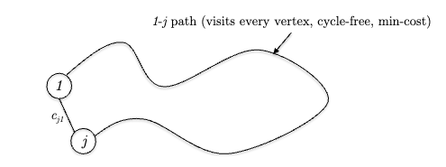
then this $1-j$ path must be a minimum cost, cycle-free path using vertices $V$. This means that:
\[\text{optimal tour cost} = \min_{j \in \{2, ..., n\}} \left( \text{min cost of cycle free 1-j path that visits $V$} + c_{j1} \right)\]
but how do we reason about the “min cost of cycle free 1-j path that visits $V$”? Realize that by a similar logic:

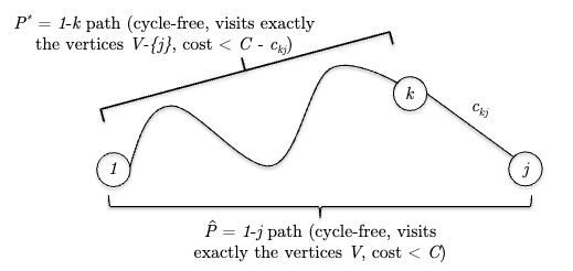
i.e. plucking off the penultimate hop $k-j$ for some $k \in V \setminus {1, j}$, we have a minimum, cycle-free path using vertices $V - \{j\}$ . (this is the tricky part, instead of being the minimum cycle-free path using vertices $V$, because enabling $j$ could give us shortcuts). Therefore, this means:
\[\text{min cost of 1-j path for $V$} = \min_{k \in \{2, ..., n\} \setminus \{j\}} \left( \text{min cost of 1-k path for $V \setminus \{j\}$} + c_{kj} \right)\]
and the above indeed can recurse into a DP algorithm.
subproblems and recursions: this leads to TSP recurrence. Let $C_{S,j}$ denote the minimum cost of a cycle-free path that visits all vertices in $S$, begins with $1$ and ends at $j$ (note beginning with a vertex $1$ is fine as the final solution is a tour). Then, for every subset $S \subset V$ that contains vertex $1$:
\[C_{S,j} = \min_{k \in S, k \neq 1,j} \left( C_{S \setminus \{j\}, k} + c_{kj} \right)\]
i.e. there are $\vert S\vert -2$ candidate solutions for an optimal path that visits all vertices in $S$ and ends at $j$, each designating a different penultimate vertex $k$ (see the figure above). Obviously, given this the final solution is:
\[\text{optimal total cost} = \min_{j \in \{2, ..., n\}} \left( C_{V, j} + c_{j1} \right)\]
until $S$ grows in size and reached $V$.

Finally, we can use this recurrence to construct a DP algorithm:

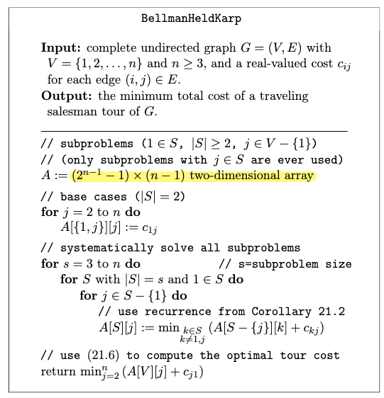
where we had

$\vert S\vert \ge 2$ because every subset $S$ must contain vertex $1$ and at least one other vertex $j$ for the “figure above to work”
base case: if there are just two vertices in $S$, and we need to find a path that starts with vertex $1$, then there is only one choice for each $C_{S,j}$.
there are in total $2^{n-1}-1$ subproblems of set $\vert S\vert \ge 2$.

Correctness of this algorithm can be proven using induction on subproblem size $\vert S\vert$.

Runtime: as for a typical DP algorith, we consider:

number of subproblems: the size of $A$, which is $(2^{n-1}-1)(n-1) = O(n 2^{n})$
time per subproblem: we still needed to do a $A[S][j] = \min (…)$, so $O(n)$
post-processing (not reconstruction): another $\min$ before we return, so $O(n)$

hence in total we get:

\[O(n 2^{n}) \times O(n) + O(n) = O(n^{2} 2^{n})\]

Note that this is still exponential, but much better than $O(n!)$.

How do we reconstruct the tour? See problem set 10.

Finding Long Paths by Color Coding

Minimum-Cost $k$-Path: given an undirected graph $G=(V,E)$ with edge costs $c_{e} \in \R$, and a positive integer $k$, find a path of length $k-1$ with minimum total cost.

if $G$ has no $k$-path, then output $+\infty$.

yes, a $k$-path can start/end at any vertex in $G$, as long as it is cycle-free and has $k-1$ edges

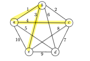
For example, in the following graph the optimal 4-path has cost 8, which is $(c \to a \to b \to e)$.

As you may have guesses, this is also NP-hard and shares many similarities with TSP. But before we go to a DP approach, what is the runtime for exhaustive search? Given a $k$:

we can iterate over all possible $k$-sized tuples of vertices
therefore, there is $n \cdot (n-1) \cdot … \cdot (n-k+1) = O(n^{k})$ tuples to check
to compute the cost of each tuple, it takes $O(k)$. So in total $O(k n^{k})$.
this is again worse than things like $O(2^{k})$, as $n$ can be very large in practice.

So how do we solve this using DP?

Attempt 1: use the same trick from The Bellman-Held-Karp Algorithm for the TSP, where we define $C_{S,v}$ as the minimum cost cycle-free path that ends at vertex $v$ and visits exactly once each vertex in $S$, for $\vert S\vert \le k$.

note that this differs from TSP where we do not require “start at vertex $1$ AND end at vertex $v$”, as we can start at any vertex

We then just need to build up the solution from $\vert S\vert =1$ to $\vert S\vert =k$, and the optimal solution will be the minimum of $\min_{S_k, v} C_{S_k, v}$ for $S_{k}$ has size $k$ and $v \in S_k$.

While this would work, but how many subproblems are there?

to choose $\vert S\vert \le k$, we have $\sum\limits_{i=1}^{k} {n \choose i} = O(n^{k})$
to scan over every $v \in S$, we have $O(k)$

so this would give $O(k n^{k})$, which is the same as exhaustive search.

Color Coding

The trick is to use color coding to track less information about a path than the full set of vertices it visits. The idea is to assign a color to each vertex, and then track the colors of the vertices visited by a path.

Given a graph $G=(V,E)$ with length bound $k$:

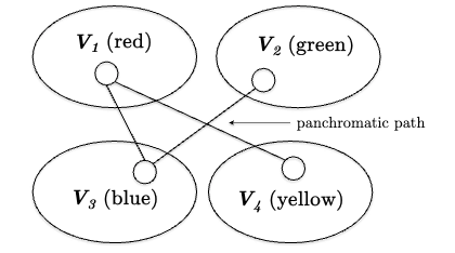
Color Coding: suppose you are given a partition of $k$ groups $V_{1} \cup V_{2} \cup … \cup V_{k} = V$ so that the minimum cost $k$-path is panchromatic, i.e. every one of the $k$ vertices reside in a different partition

Why is this useful? The plan is this:

we can later show that with some randomized calls, we WILL eventually get a “lucky enough” partition where the optimal $k$-path is panchromatic

given the path is panchromatic, we find it much quicker than exhaustive search

For example, consider the following graph with $k=4$, where we can imagine each partition having a different color:

Computing a Minimum-Cost Panchromatic Path

Now you will see why this is faster, as instead of iterating over all possible $k$-sized tuples of vertices (which has $O(n^{k})$ subproblems), we can instead iterate over all possible $k$-sized tuples of colors:

\[\sum\limits_{i=1}^{k} {n \choose i} = O(n^{k}) \quad \to \quad \sum\limits_{i=1}^{k} {k \choose i} = O(2^{k})\]

since each subproblem now only needs to consider a path that visits $\le k$ vertices of different colors (assuming that the optimal path is panchromatic). Now, all we need to do is to redefine the subproblems and recursion using colors.

Let $C_{S,v}$ denote the minimum cost of an $S$-path that ends at some vertex $v$, and visits exactly once each color in $S$, for $S \subseteq {1,2, … ,k}$. Let $\sigma(v)$ denote the color of vertex $v$.

optimal solution’s structure: essentially the same as TSP where we can pluck the last vertex out, along with its color:

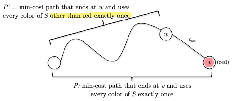
note that we do not have a start vertex here, and the smaller subproblem represents having one less color to visit (which skips a LOT of subproblems)!
subproblems and recurrence: again building from bottom up, for every subset $S \subseteq {1,2, … ,k}$ and every vertex $v \in V$:
\[C_{S,v} = \min_{(w,v) \in E} \left( C_{S \setminus \{\sigma(v)\}, w} + c_{wv} \right)\]
where there are a couple differences from TSP:
- we still need to check every vertex $v \in V$ to build up the solution, but after checking one $v$ we can throw out all vertices of the same color $\sigma(v)$
- since this is looking for a path, we just need to check $(w,v) \in E$.
The final optimal solution is then:
\[\min_{v \in V} C_{\{1,2, ... ,k\}, v}\]
where $S={1,2, … ,k}$ is the full set of colors.

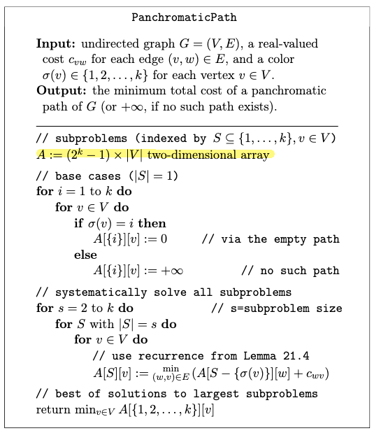
Hence our DP algorithm is:

again, this assumes that the optimal path is panchromatic.

Correctness: induction by problem size on $\vert S\vert$

Runtime: here the main cost is in the triple for loop:

to compute $A[s][v] = \min(…)$ it takes $O(\mathrm{degree}(v))$ time
to compute for v in V then takes $O(\sum\limits_{n\in V} \mathrm{degree}(v)) = O(2m)=O(m)$ time
since then it just iterates over all possible $S \subseteq {1,2, …, k}$, we get $O(2^{k} m)$ time

This is great as it is much better than $O(n^{k})$, but what do we do about the “lucky case” of the optimal path being panchromatic?

Randomized Color Coding

The idea is that perhaps with a uniformly randomly colored graph, we can eventually get lucky enough to find a panchromatic path.

Suppose we uniformly assign a color ${1, …, k}$ for each vertex at random. What is the probability that a given $k$-path is panchromatic?

there are in total $k^{k}$ possible colorings for that $k$-path
being panchromatic means that each color is used exactly once, so there are $k!$ ways to do that
therefore, the probability of being panchromatic is $k! / k^{k}$

How big is it? Now we can use steriling’s approximation to better see:

\[p = \frac{k!}{k^{k}} \approx \frac{\sqrt{2 \pi k}\left(\frac{k}{e}\right)^{k}}{k^{k}} = \frac{\sqrt{2\pi k}}{e^{k}}\]

with $k=7$ this number is already less than 1% due to the exponential term. But we don't need to get this done in one-shot. All we need is to be lucky for once in a reasonable number of trials. So what is the probability of getting at least once panchromatic path in $T$ trials?

this is equivalent to $1 - (1-p)^{T}$, where $p$ is computed above as the probaility of success in one trial, hence $(1-p)^{T}$ is the chance that all $T$ trials were unlucky
to compute this, consider bounding $1-p$ from above by $e^{-p}$, which works because:

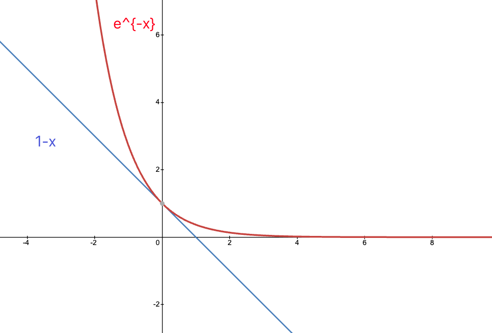
therefore we get:
\[(1-p)^{T} \le (e^{-p})^{T} = e^{-pT}\]

And therefore for a failure rate smaller than $\delta=0.01$, i.e. failure rate of 1%, we can set:

\[e^{-pT} \le \delta \implies T \ge \frac{1}{p} \ln \frac{1}{\delta} \approx \frac{e^{k}}{\sqrt{2\pi k}} \ln \frac{1}{\delta}\]

This gives our final algorithm of color coding with randomized trials:

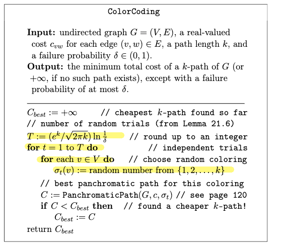
where basically in the yellow part you just recolor everything for $T$ trials. This gives the total runtime of:

\[O\left( e^{k} \ln \frac{1}{\delta} \right) \times O(2^{k} m) = O\left( (2e)^{k} m \ln \frac{1}{\delta} \right)\]

which gives probability of success (i.e. reaching the lucky case of optimal path being panchromatic) at least $1-\delta$.