COMS4733 Computational Aspects of Robotics
- Logistics:
- Introduction to Robotics
- Rigid-Body Transformations
- Configuration Space
- Kinematics
- Search-Based Planning
- Dynamic Replanning
- Combinatorial Motion Planning
- Probabilistic Roadmaps
- Single-Query Planners
Table of Contents:
[toc]
Logistics:
- Will be quite heavy in math: linear algebra + probability and stats
- Textbooks: Principle of Robot Motion (mostly), Planning Algorithms
- OH: 712 CEPSR, details posted on Edstem Live Calendar
- Grades: HW 40%, Midterm 30%, Final 30%
Introduction to Robotics
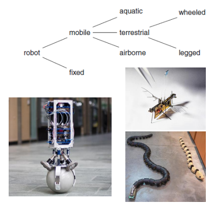
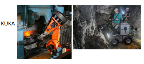
Robots can be classified into many categories by various methods:
-
one way of classification: | Manipulator | Mobile | Humanoid | | :————————————————————————————————: | :————————————————————————————————: | :————————————————————————————————: | |
 |
|  |
| 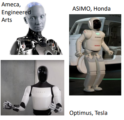 |
|where manipulators are often fixe in place and used in industry a lot (e.g., warehouses), mobile robots tend to interact with dynamic and unknown environments (e.g., self-driving cars), and humanoid robots are mainly designed to assist and interact humans
-
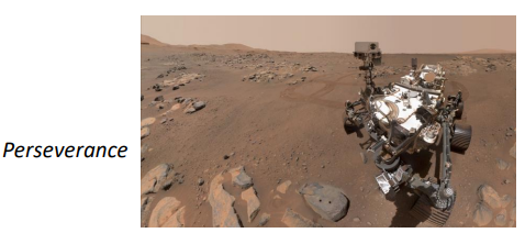
or we can classify them by functions: | Industrial | Field | Service | | :————————————————————————————————: | :————————————————————————————————: | :————————————————————————————————: | |
 |
|  |
| 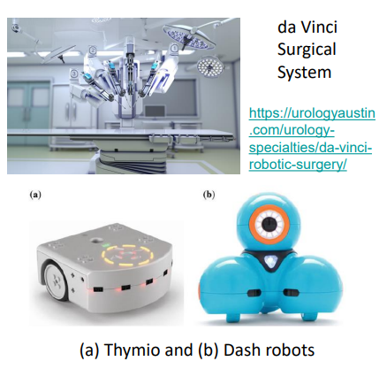 |
|where industrial robots are often pre-programmed, field robots need to operate in unstructured environments, and service robots are designed to assist humans in daily life
What kinds of computation problems do we care about in robotics?
- How do you represent and model your robot and its environment? (so that you can easily compute things)
- How do you control your robot?
- robot kinematics: if you moved a joint by this bit, how much does the end-effector move?
- motion planning and automation
- Robot sensors have a lot of noises. Need estimation, localization, and mapping to perceive what is happening in the environment
- AI learning and perception
Rigid-Body Transformations
Let the world be represented with $\mathcal{W}$, and let a subset of points $\mathcal{A}$ be what we interested in (e.g. obstacles, our robot, etc)
We will also typically use coordinates relative to either a fixed world frame, or fixed robot’s body frame.
Rigid-body transformation: A transformation function $h: \mathcal{A} \to \mathcal{W}$ such that relative distance and orientations between all points in $\mathcal{A}$ are preserved (i.e., your robot is not stretching itself, and is not “flipping” itself). Examples include:
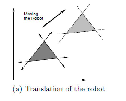
- translations
- rotations
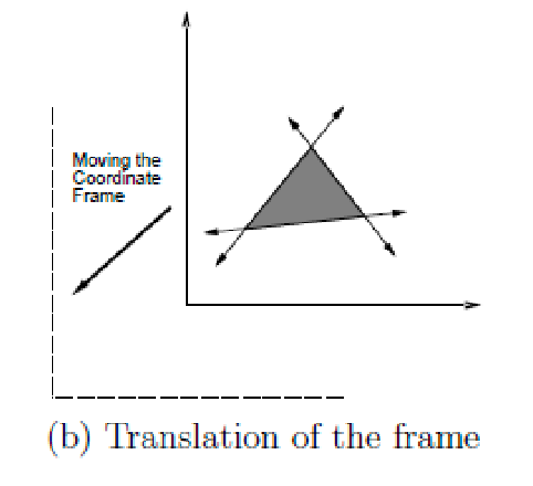
A 2D translation by $\mathbf{p} = (x_t, y_t)$ applied to all points in $\mathcal{A}$
\[h(x, y ) = (x+x_t, y+y_t)\]this can be interpreted in two ways:
| you transformed the points in the robot | you transformed the origin of the frame |
|---|---|
 |
 |
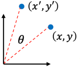
A 2D rotation: suppose we rotate our robot counter-clockwise about the origin of the world frame by an angle $\theta$. You can do this
| Visually | Mathematically |
|---|---|
 |
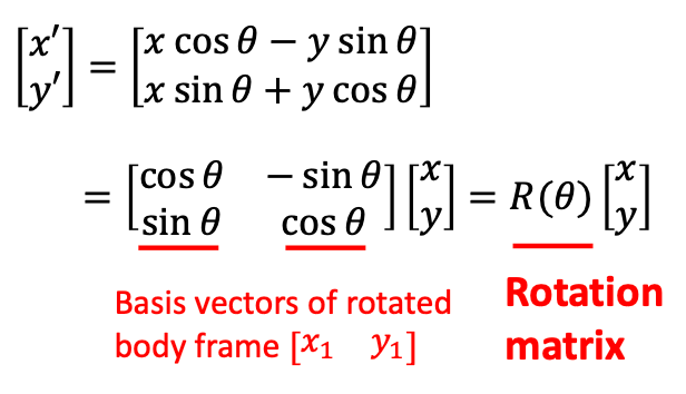 |
so now your function becomes:
\[h(\mathbf{x}) = R(\theta) \mathbf{x}\]in fact, there is a simple interpretation of this rotation matrix:
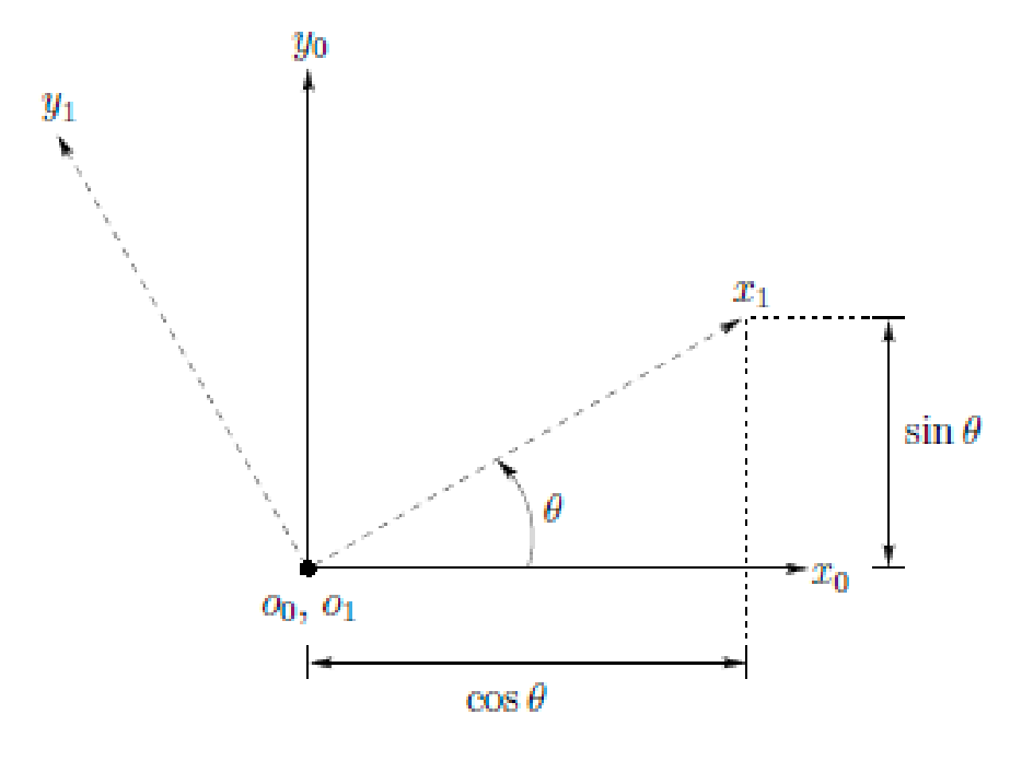
The first column of $R$, which is $[\cos \theta, \sin\theta]^T$, is the coordinate of $x_1$ w.r.t the old frame, and the second columd is the coordinate of $y_1$ w.r.t the old frame! So the operation of:
\[\begin{bmatrix} \cos\theta & -\sin\theta \\ \sin\theta & \cos \theta \end{bmatrix} \begin{bmatrix}x \\ y\end{bmatrix} = x \begin{bmatrix} \cos\theta \\ \sin\theta \end{bmatrix} + y \begin{bmatrix} -\sin\theta \\ \cos\theta \end{bmatrix}\]so it is basically the “same $(x ,y)$” but in a new coordinate frame!
Properties of Rotation Matrix: a rotation matrix is quite important, and it has a lot of useful properties:
- $R(\theta)$ produces a counter-clockwise rotation
- it is orthogonal: $R(\theta)^{-1} = R(\theta)^T$
- additional $R(\theta)^{-1} = R(-\theta)$, so inverse is just a clockwise rotation
- $\det(R(\theta)) = 1$, so rotation does not change length, size, or magnitude (i.e., does not stretch points, rigid-body transformation!)
- is composable $R(\theta_1 + \theta_2) = R(\theta_1)R(\theta_2)$
- 2D rotation transformation is communicative (but not for 3D) $R(\theta_1)R(\theta_2) = R(\theta_2)R(\theta_1)$
- rotation matrices represent rotation as linear transformations
Homogenous Transformations
Now you can combine rotaion and translation:
\[\begin{bmatrix}x' \\ y'\end{bmatrix} = R(\theta) \begin{bmatrix}x \\ y\end{bmatrix} + \begin{bmatrix}x_t \\ y_t\end{bmatrix}\]is a valid rigid body transformation, but is now affine, not linear transformation. Some common trick to make this a linear transformation (so math is simpler later) is to add a dimension $(x,y) \to (x,y,1)$:
\[\begin{bmatrix} x' \\ y' \\ 1 \end{bmatrix} = \begin{bmatrix} \cos \theta & -\sin \theta & x_t \\ \sin \theta & \cos \theta & y_t \\ 0 & 0 & 1 \end{bmatrix} \begin{bmatrix} x \\ y \\ 1 \end{bmatrix} = T(\theta, x_t, y_t) \begin{bmatrix} x \\ y \\ 1 \end{bmatrix}\]so that both rotation and translation is expressed as a homogeneous linear transformation (in 2D space). This turns out to be a general form:
Homogenous Transformation Matrix: this form generalizes if you are doing rotations and translations only:
\[T(\theta, x_t, y_t) = \begin{bmatrix} \cos \theta & -\sin \theta & x_t \\ \sin \theta & \cos \theta & y_t \\ 0 & 0 & 1 \end{bmatrix} = \begin{bmatrix} R(\theta) & \mathbf{p} \\ \mathbf{0}^T & 1 \end{bmatrix}\]so for example:
to do pure rotation, substitute $\mathbf{p}=[0,0]^T$, and for pure translation, substitute $R(\theta) = I$
no longer orthogonal, so inverse is a bit more compllicated
\[T^{-1} = \begin{bmatrix} R^-1 & -R^{-1}\mathbf{p}\\ \mathbf{0}^T & 1 \end{bmatrix}\]not commutative: $T_1 T_0(x,y,1) \neq T_0 T_1(x,y,1)$
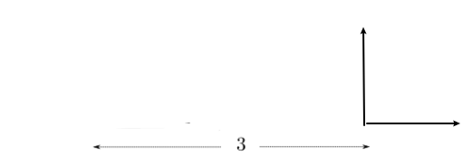
For example, consider visually what would happen if I do $T_0$ being pure rotation by $\pi/4$, and $T_1$ being translation to right by $3$
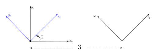
| Step 0 | Step 1 | Step 2 |
|---|---|---|
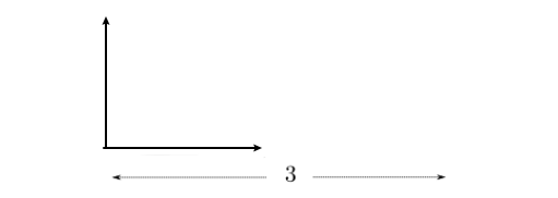 |
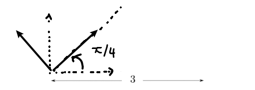 |
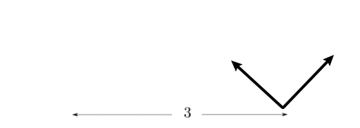 |
If you do in reverse order
| Step 0 | Step 1 | Step 2 |
|---|---|---|
|
 |
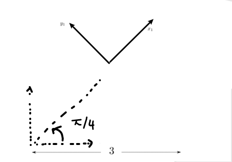 |
note that all intermediate transformations are relative to the original frame.
3D Transformations
Essentially the same idea as 2D transformations, but:
-
3D translations are still simple: $h(x,y,z)=(x+x_t, y+y_t, z+z_t)$
-
3D rotations is much more complicated because you can rotate relative to many axis
-
e.g., rotation around the $z$-axis
\[R_z(\alpha) = \begin{bmatrix} \cos \alpha & -\sin \alpha & 0\\ \sin \alpha & \cos \alpha & 0 \\ 0 & 0 & 1 \end{bmatrix} \to \begin{bmatrix} \mathbf{x_1} & \mathbf{y_1} & \mathbf{z_1} \end{bmatrix}\]and again, the interpretation is the same as before: rotation matrix describes the new coordinate axis
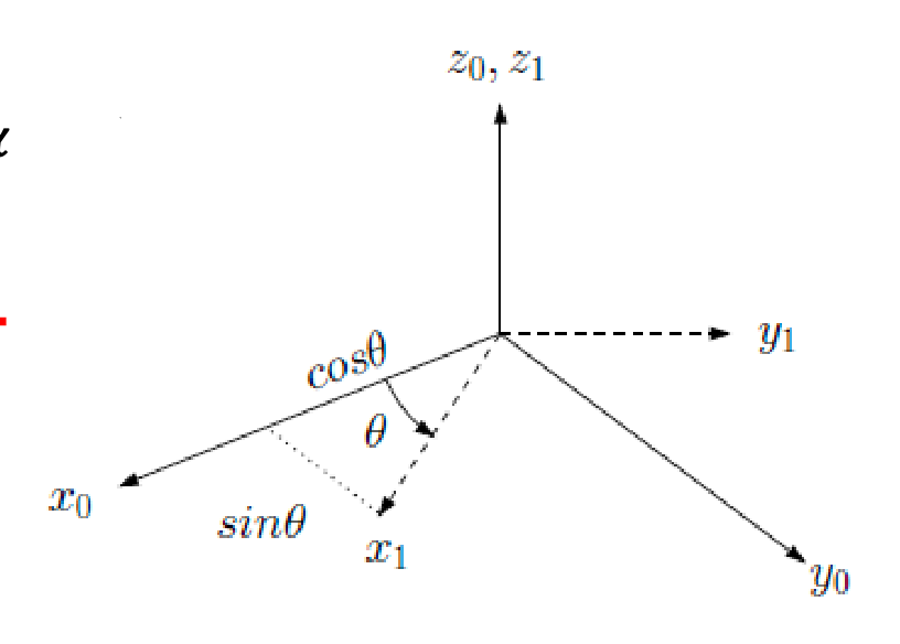
notice that:
-
the zeros and ones is intuitive: since $z$-axis isn’t moving, they have to appear like this!
-
and the upper part of this matrix is exactly the same as the 2D transformation matrix $R(\theta)$
-
-
e..g, since you have three axis, you have two more rotation matrices
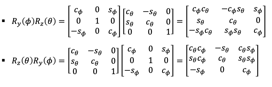
\[R_y(\beta) = \begin{bmatrix} \cos \beta & 0 & \sin \beta \\ 0 & 1 & 0 \\ -\sin \beta & 0 & \cos \beta \end{bmatrix},\quad R_x(\gamma) = \begin{bmatrix} 1 & 0 & 0 \\ 0 & \cos \gamma & -\sin \gamma \\ 0 & \sin \gamma & \cos \gamma \end{bmatrix}\] -
right-hand-rule: a 3D “positive rotation” by $\theta$ about some axis $\mathbf{v}$ is a counter-clockwise rotation in the plan normal to $\mathbf{v}$. Visually, it is just right-hand-rule:
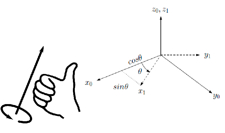
-
rotations about the same axis is commutative (as in 2D), but not commutative when you are rotating about different axes (in 3D)
-
but each 3D rotation matrix is orthogonal
-
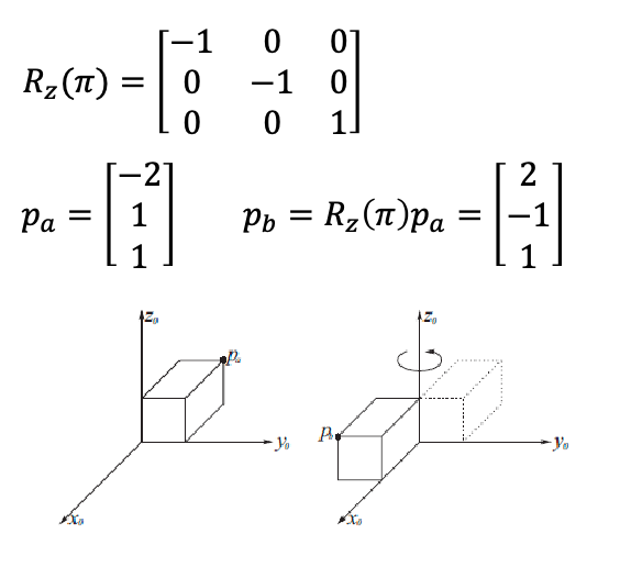
For example, consider our “robot” is a box, and we want to transform all points of this box by $\pi$ in the $z$-axis (let us just visualize one point of the box):
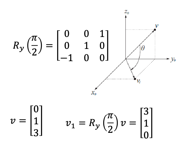
For example: transform a vector $\mathbf{v}$ by $\pi/2$ in the $y$-axis
3D Homogeneous Transformations
Similar to 2D, if we do one rotation and and one translation: we can make it into one linear transformation matrix by uplifting one dimension.
For example, rotating about $y$-axis by $\beta$ followed by a translation:
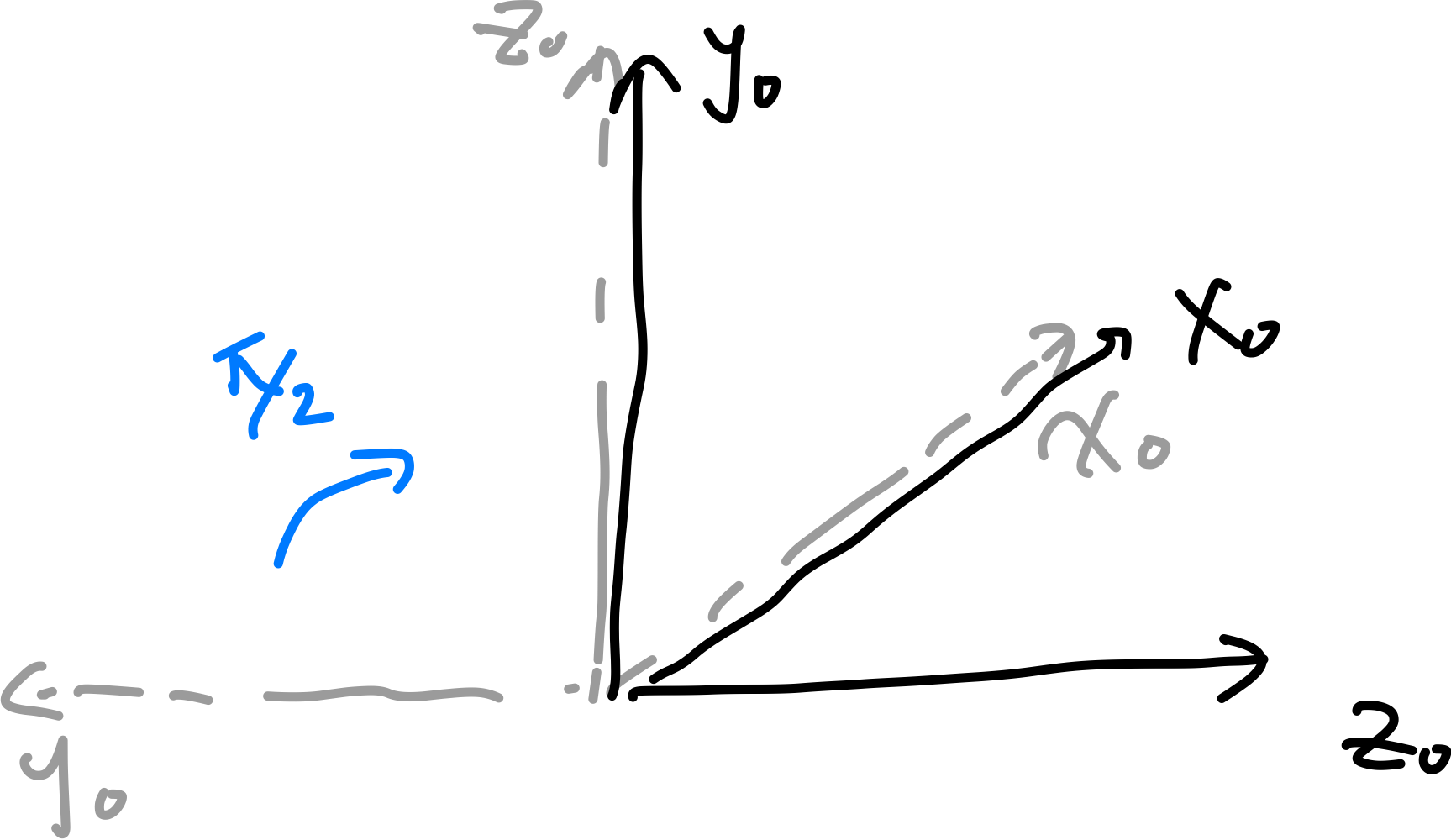
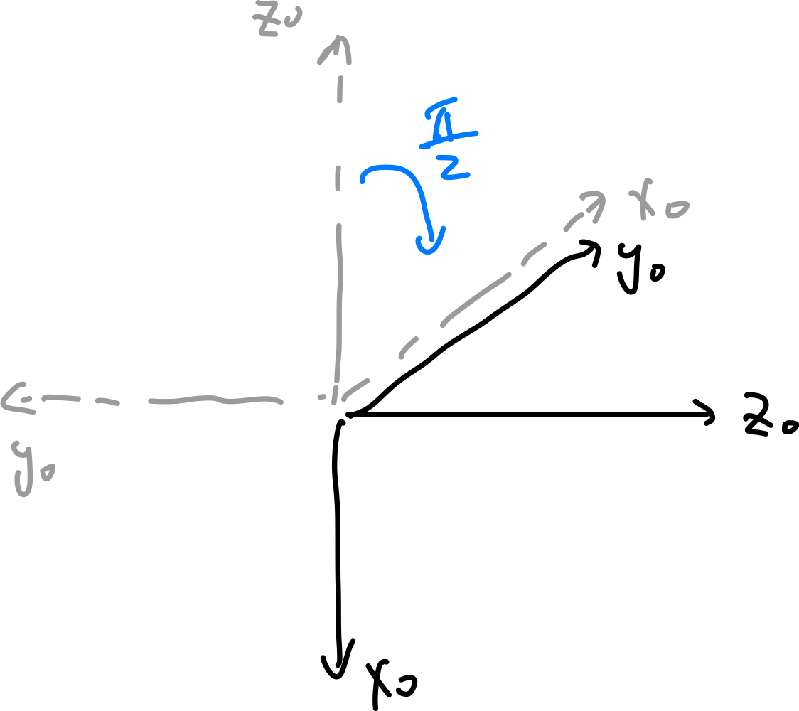
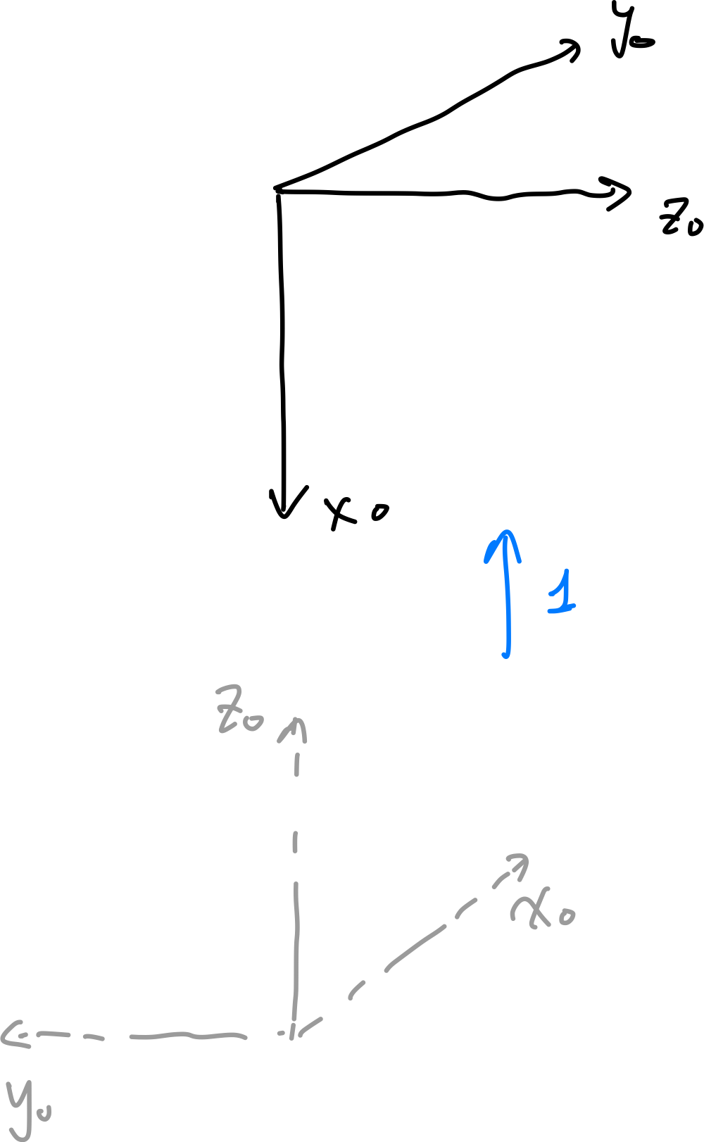
\[T = \begin{bmatrix} R_y(\beta) & \mathbf{p} \\ \mathbf{0}^T & 1 \end{bmatrix} = \begin{bmatrix} \cos \beta & 0 & \sin \beta & x_t \\ 0 & 1 & 0 & y_t \\ -\sin \beta & 0 & \cos \beta & z_t \\ 0 & 0 & 0 & 1 \end{bmatrix}\]As an exercise, try to figure out the transformation matrix from frame 0 to frame 1, and then from frame 1 to frame 2:
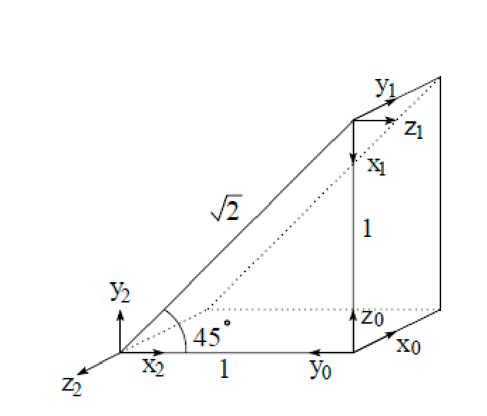
-
from frame 0 to frame 1: we are rotating about $x_0$ by $\pi/2$, rotate about $y_0$ by $\pi/2$, and translate along $z_0$ by 1unit
Step 0 Step 1 Step 2 Step 3 
therefore the full transformation matrix look like:
\[T_1^0 = \begin{bmatrix} I & [0,0,1]^{T} \\ \mathbf{0}^T & 1 \end{bmatrix} \begin{bmatrix} R_{y}(\pi/2) & \mathbf{0} \\ \mathbf{0}^T & 1 \end{bmatrix} \begin{bmatrix} R_{x}(\pi/2) & \mathbf{0} \\ \mathbf{0}^T & 1 \end{bmatrix} = \begin{bmatrix} 0 & 1 & 0 & 0 \\ 0 & 0 & -1 & 0 \\ -1 & 0 & 0 & 1 \\ 0 & 0 & 0 & 1 \end{bmatrix}\]note that in this case
- each column represents the new coordinate’s axis relative to the original frame! (e.g., $x_1$’s coordinate is exactly pointing at $[0,0,-1]$, and the new origin at $[0,0,1]$ from the last column).
- Also note that we do translation last, since it is the simplest as all transformation (i.e., the rotations) are relative to the original frame.
- we denote $T^0_1$ means we are transforming from frame 0 to frame 1
-
from frame 1 to frame 2: left as an exercise
Composition Ordering
But what if I already give you the transformation of $T^0_2$?
\[T_2^0 = \begin{bmatrix} 0 & 0 & -1 & 0\\ -1 & 0 & 0 & 1 \\ 0 & 1 & 0 & 0 \\ 0 & 0 & 0 & 1 \end{bmatrix}\]Can you tell me what is $T^1_2$ given this information and your previous result of $T^0_1$?
-
attempt 1: can say that:
\[T^1_2 \overset{?}{=} T^0_2 T^1_0 = T_2^0 (T^0_1)^{-1}\]No, because the two transformations are done in different basis. The first transformation $T^1_0$ is based on frame 1, and the second $T^0_2$ is based on frame 0!
-
attempt 2: we need to write $T^{0}_2$ transformation relative to frame 1. This is a similarity transformation:
\[T^0_2 \to (T^0_1)^{-1} T^0_2 (T^0_1)\]Therefore, the correct transformation is:
\[T^{1}_2 = (T^0_1)^{-1} T^0_2 (T^0_1) (T^0_1)^{-1} = (T^0_1)^{-1} T^0_2 = T^{1}_0 T^{0}_2\]and note that this is almost the same as the first attempt, but flipped!
This turns out to be turn in general. Consider two homogenous transformations $A,B$:
- if both are written relative to the same frame, then you can simply combine them and the result is intuitive. E.g., $C=BA$ transformation means you first do $A$ and then $B$.
if they are not written relative to the same frame, for example $A=T^{i}_j$ is w.r.t. frame $i$ and $B=T^{j}_k$ is w.r.t. frame $j$, then:
\[T^{i}_j T^{j}_k = T^{i}_k\]is transforming from frame $i$ (left matrix) to frame $k$ (right matrix).
So in some sense, you can say “absolute transformations” (same frame) are pre-multiplied (right to left), and “relative transformations” (different frame) are post-multiplied (left to right).
Configuration Space
Configuration: Description of the positions of all points of a robot
Configuration Space (C-Space): the space of all possible configurations of the robot.
- In theory, there may have an infinite list of point positions, but in practice we consider parameterized representations of C-space
Group $(G, \circ)$ is a set $G$ with binary operatoin $\circ$ such that for all $a,b,c\in G$:
- Closure: $a\circ b \in G$
- Associativity: $(a\circ b) \circ c = a \circ (b \circ c)$
- Identity: $\exists e \in G$ such that $e \circ a = a \circ e = a$
- Inverse: $\forall a \in G$, $\exists a^{-1} \in G$ such that $a \circ a^{-1} = a^{-1} \circ a = e$
For example, $(\Z, +)$ is a group, where of course adding two integers still gives an integer, etc. Alternatively, the group $(\R - {0}, \times )$ also works. Note that zero is taken out since it does not have multiplicative inverse.
General Linear Group: the set of all non-singular (non-zero determinant) $n\times n$ real matrices with the operation of matrix multiplication.
We are interested in this group because some subgroups of this are useful to robotics. For example:
- Orthogonal group $O(n)$, a set of $n\times n$ orthogonal matrices with $\det = \pm 1$
- Special Orthogonal Group $SO(n)$, subgroup of $O(n)$ with $\det = +1$. Any matrix in $SO(n)$ will corresponds to a $n\times n$ rotation matrices we saw before.
- Special Euclidean Group $SE(n)$, a set of $(n+1)\times (n+1)$ homogeneous transformation matrices in $\mathbb{R}^n$. The rigid-body transformations are a subset of this, since we also require no-stretching.
C-Space of Mobile Robots
Positions of robot = uniquely defined by a transformation matrix (plus a given original position) Configuration of a robot: a complete specification of the position of every point of the system. We will use $q$ to denote a configuration.
Configuration Space (C-Space): space of all possible configurations of the robot. We will use $\mathcal{Q}$ to denote the C-space.
Degree of Freedom of a robot system is number of parameters needed to specify a configuration, or the dimension of the C-space.
For example, a circular, 2D robot with a known radius $r$ can be fully described using the location of its center. Therefore, a configuration looks like $q=(x,y)$, which has two degrees of freedom. The C-space has dimension 2, and is just $\R^2$ in this case.
We can also tie this back to the groups we discussed before. We can say single body robots can be described by $SE(2)$ or $SE(3)$. This is because any configuration of a single body robot can be described by a transformation matrix in $SE(2)$ or $SE(3)$, and these group of matrices contain all possible translations and rotations in 2D or 3D space.
For example:
- if the robot only translates, then often its C-space is just $\R^{2}$ or $\R^{3}$
- if the robot only rotates, then we can say its C-space is $SO(2)$ or $SO(3)$
- if we have multiple robots, then the full C-space is the Cartesian product of each body’s individual C-space
We can also describe the degrees of freedom of those matrix groups, interpreted as the number of parameters needed to construct them:
- $SO(2)$ and $SO(3)$ have dimension 1 and 3, respectively (for 3D, worst case you can have one rotation from each three axis)
- $SE(2)$ corresponds to $\R^2 \times SO(2)$, which has dimension $2+1=3$
- $SE(3)$ corresponds to $\R^3 \times SO(3)$, which has dimension $3+3=6$
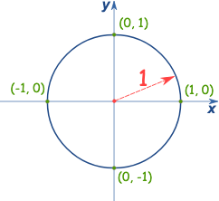
Unit Circle
Since $SO(2)$ has dimension 1, what’s the difference with $\R^1$? Realize that $SO(2)$ is uniquely parametrized by value $[0, 2\pi)$. To visualize this space, we can consider the points on a unit circle:
\[\mathbb{S}^{1} = \{ (x,y) \in \R^2 | x^2 + y^2 = 1 \}\]and note that each point on the unit circle maps to a value in $[0, 2\pi)$ (so its a good way to visualize it). More formally:
Homeomorphism: $SO(2)$ and $\mathbb{S}^1$ are homeomorphic, since there exists a continuous bijection function $f:X\to Y$
- i.e., so that you can visualize these two sets (of free variables) as the same thing
This “visualization” tool comes in handy later when things get complicated.
Kinematic Chains
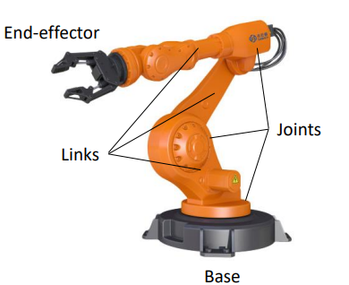
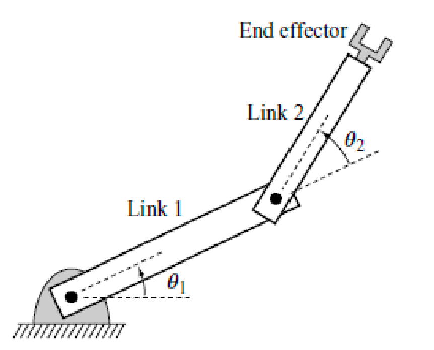
Can we describe the C-space of a manipulator? For a manipulator, each rigid body has a link, and links are connected by joints:
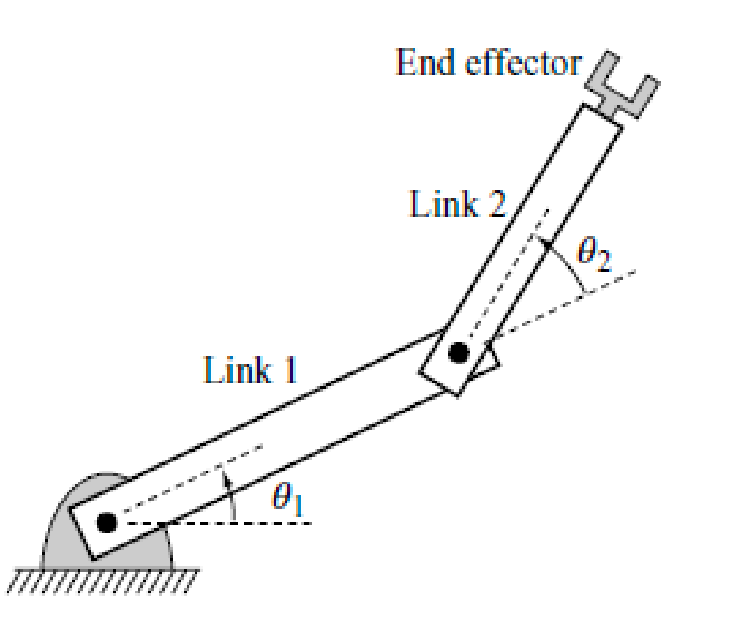
What’s interesting now is that since each joint only has one degree of freedom, it severly restricts the degree of freedom of links and end effector. This means that two fully describe the C-space of this robot, we only have two degrees of freedom: $(\theta_1, \theta_2)$.
More formally, the C-space is (not $\R^2$):
\[\mathbb{S}^1 \times \mathbb{S}^1\]How do you “visualize” this C-space? This is actually homeomorphic to the surface of a 2D torus $\mathbb{T}^2$.
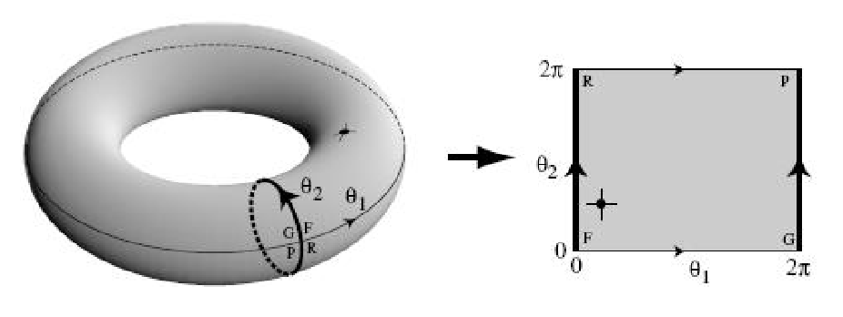
where every point on the surface of the 2D torus corresponds to a unique angle configuration we have.
Manifolds
Even though $\mathbb{S}^1$ and $\R$ are not homeomorphic and topologically different, they are locally similar.
Manifold: A subset $M \subseteq \R^m$ is a $n$-dimension manifold if each point in $M$ lies in a neighborhood that is homeomorphic to an open subset of $\R^n$
- i.e., we can locally flatten each point in $M$, so that it is homeomorphic (can map) to $\R^n$
- e.g. a globe (Earth) is a manifold since the neighbor area we see are basically flat
Practically, a valid manifold means you have a valid mapping $f:X\to Y$ with an inverse $f^{-1}:Y\to X$, where the space of $Y \in M$ and $X$ is in your original space.
For example, $\mathbb{S}^1$ is a 1-dimensional manifold in $\R^2$
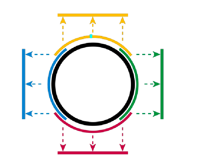
-
this is because we can have a mapping where blue and green does $(x,y) \to y$, and yellow and red does $(x,y)\to x$.
- notice that the mapping is unique within the neighborhood
- so “1-dimensional manifold in $\R^2$” means $\mathbb{S}^1$ lives in $\R^2$ as shown above, but we can flatten it in a way to describe it using only one continuous number (i.e., 1-dimensional manifold)
For another example, the following are 2-dimensional manifolds in $\R^3$:
- $\mathbb{S^2}$ the surface of a sphere
- $\mathbb{T^2} = \mathbb{S^1} \times \mathbb{S^1}$ the surface of a torus
- $\R \times \mathbb{S^1}$ infinite cylinder
Matrix Lie Groups
Lie Groups: groups that are also (differentiable) manifolds.
- this includes $SE(n)$ and its subgroups, and most robot related C-spaces
- basically now, we are visualizing “matrix groups” as “manifolds”
For example, a real $n\times n$ matrix is trivially homeomorphic to $\R^{n^2}$:
\[A = \begin{bmatrix} a & b \\ c & d \end{bmatrix} \iff (a,b,c,d)\]where in this example, $SE(2)$ is homeomorphic to $\R^4$.
What about matrices in $SO(2)$? Even though this is $\mathbb{S}^{1}$, we know we can flatten it to a 1-dimensional manifold in $\R^2$. So we can say $SO(2)$ is homeomorphic to $\R$. Another more direct way to think about this: $\mathbb{S}^{1}$ describes the points on a unit circle, which can be “flattened” into a manifold.
Obstacles as Polygons
Real robot C-spaces are often not just an “open-world” $\mathcal{W}$, there may be obstacles $\mathcal{O}_i \in \mathcal{W}$.
A robot’s workspace is the subset two or three-dimensional Euclidean space $\mathcal{W}$ that it can reach.
To efficiently represent this space, we will consider two tricks:
- represent $\mathcal{O}$ using a combination of primitives (e.g., intersection of lines, planes)
- then we can directly “transform” these primitives into the C-space of the robot = robot’s free C-space
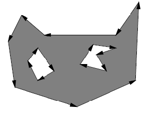
As a starting point, consider a simple 2D obstacle that we can represent with a finite set of vertices:

We can describe using line equations + inequalities:
\[O = H_{1} \cup H_{2} \cup ... \cup H_{m}\\ H_i = \{ (x,y) \in \mathcal{W} | f_i(x,y) \le 0 \}\]notice that a line equation is just $f_i(x,y) = ax + by + c = 0$, and we can use inequalities to describe the half-space of the line.
We can then describe a non-convex polygon by decomposing it into unions of convex polygons, and use set differences for holes.
This idea is similar in 3D, where we just use polyhedra = using plane equations instead of line equations, and then consider the intersection of inequalities:
We can finally generalize this even further to non-linear primitives. For example, we can use polynomial equations to represent the following:
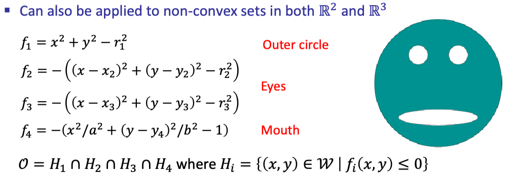
where the green area basically is the obstacle.
C-Space Obstacles
Now we want to transform those obstacles into the C-space of the robot, i.e., we want to directly obtain a single, constrained C-space.
Let $\mathcal{A}$ be our robot, and let $q \in \mathcal{Q}$ denote the configuration of $\mathcal{A}$
C-space obstacle region: is the region when the robot takes this configuration (i.e. transformation), it collides with some obstacle.
\[Q_{\mathrm{obs}} = \{ q \in \mathcal{Q} | \mathcal{A}(q) \cap O \neq \empty \}\]Free C-space: when the robot will not collide:
\[Q_{\mathrm{free}} = Q - Q_{\mathrm{obs}}\]
For example, for a 2D robot, you can imagine $q=(x_t,y_t, \theta)$, and $Q_{\mathrm{obs}}$ would be all the configurations (i.e., transformations) such that the robot will hit an obstacle after performing it.
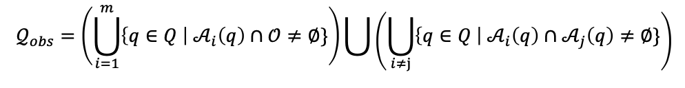
What if you have multiple bodies? Then you also need to exclude collisions between these bodies. So $Q_{\mathrm{obs}}$ is:
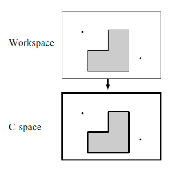
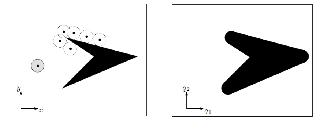
For example, visualizing free C-space if your robot is just a point (has no rotation)
Again no rotation, but if we give it some volumes:
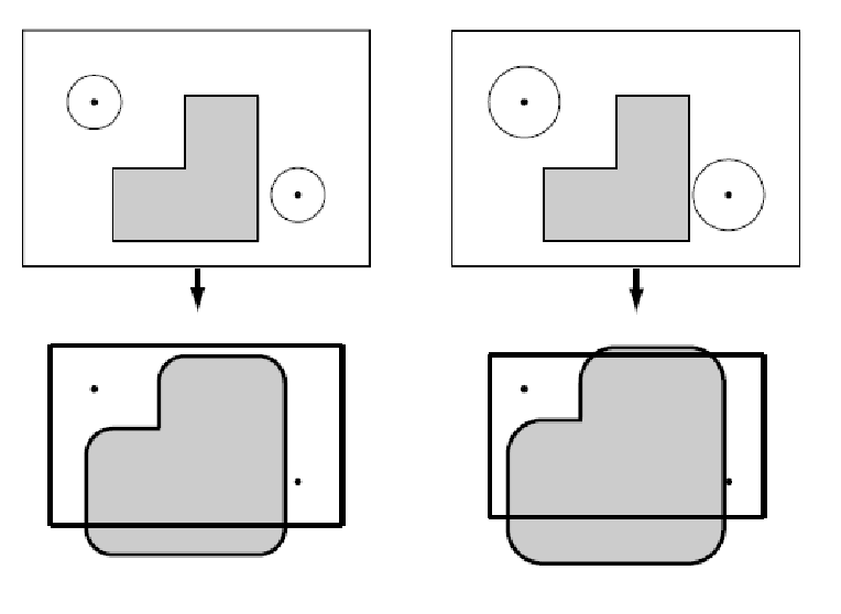
where notice that:
-
a coordinate $q$ in free C-space corresponds to a configuration (or transformation) such that $\mathcal{A}(q)$ does not hit an obstacle in the workspace.
-
in the special case here we have only two degrees of freedom (no rotation), we only needed to grow boundaries of $Q_{\mathrm{obs}}$ by the radius of the robot to obtain $Q_{\mathrm{free}}$.
-
Things get more complicated when it goes to 3D.
Minkowski Difference
Since it gets complicated in 3D quickly, but is there a simple way to figure out the obstacle space? When the robot is a rigid body restricted to translation only, we can use
Minkovski Differece: when $\mathcal{Q} = \R^{n}$, then $Q_{\mathrm{obs}}$ is the Minkowski difference:
\[\mathcal{O} \ominus \mathcal{A}(0) = \{ o - a \in \R^n | o \in \mathcal{O}, a \in \mathcal{A}(0) \}\]where $A(0)$ means the robot is at the origin, and $\ominus$ is the Minkowski difference operator. This is basically considering all points as vectors, and doing a vector minus for all possible points.
Visually
| Example 1 | Example 2 |
|---|---|
 |
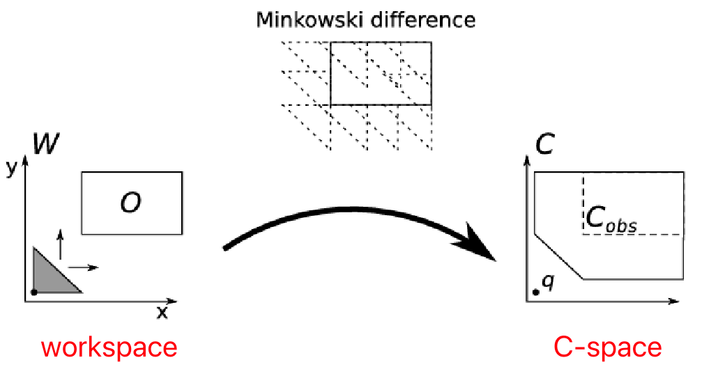 |
effectively we are obtaining the region by “sliding our robot” along the edge of the obstacles, therefore:
- the vector minus is because we need to flip our robot to slide along the edge
- the Minkowski difference considered all vectors of the robot = the shape of the robot
However, computationally this would need adding infinite number of vectors, so there are a few work-arounds
Convex Hulls
If we are dealing with convex polygons, it turns out adding/subtracting the vertices are sufficient.
The convex hull of the Minkowski differnce is the set of vertices of the C-shape obstacle region:
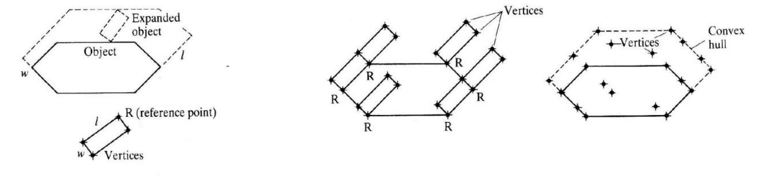
note that we won’t need to know how to implement this in $\mathcal{O}(n \log n)$, as they are many existing algorithm implementations that does this efficiently.
Star Algorithm
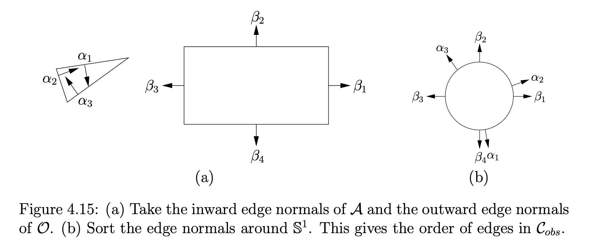
Again, If both $\mathcal{A}$ and $\mathcal{O}$ are convex, we can compute $Q_{\mathrm{obs}}$ by considering only vertex-edge contacts.
The key observation is that every edge of $\mathcal{C}_{obs}$ is a translated edge either from $\mathcal{A}$ or $\mathcal{O}$, In fact, every edge from $\mathcal{O}$ and $\mathcal{A}$ is used exactly once in the construction of $\mathcal{C}_{obs}$:
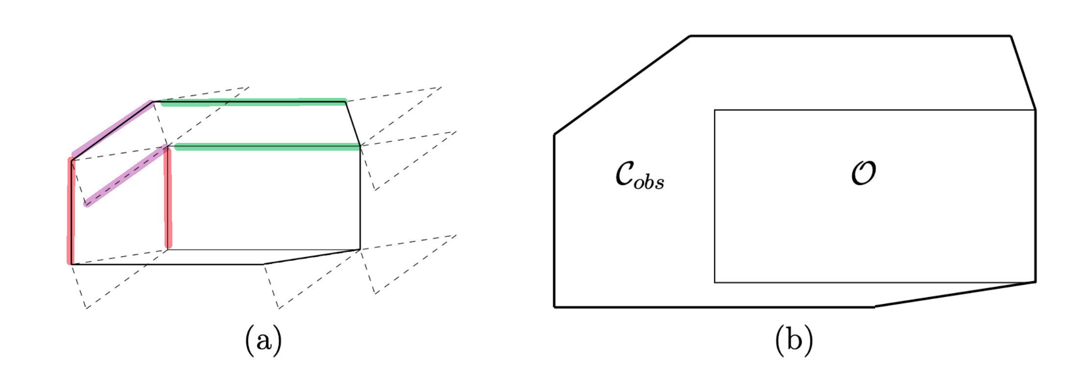
where in (a) we color-coded a couple of examples, and (b) shows the final $\mathcal{C}{obs}$. There is a translation of the edges, but that doesnt matter as we can construct if we know the order of edges to construct $\mathcal{C}{obs}$ (then we can just glue them in order).
Star Algorithm: the order of edges can be obtained by sorting:
- find the inward edge normals of $\mathcal{A}$
- find the outward edge normals of $\mathcal{O}$
- sort the edges by angle around $\mathcal{S}^1$
- Then, assemble by simply gluing edges in the order of the sorted list.
For example, to obtain the $\mathcal{C}_{obs}$ above:
| Algorithm | Glueing |
|---|---|
 |
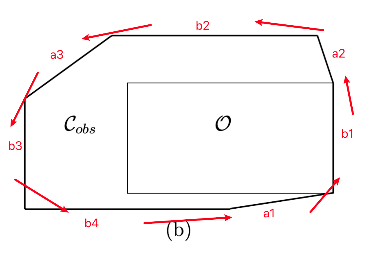 |
note that
-
this assumes the “origin” of the robot is at the top left of the robot. If not, we can simply translate $\mathcal{C}_{obs}$ by the same amount
- Star-algorithm is very fast: is linear in the number of edges of $\mathcal{A}$ and $\mathcal{O}$
- similar ideas for $\R^{3}$ based on enumerating contacts between convex polyhedra vertices and faces to obtain $\mathcal{C}_{obs}$
C-Spaces with Orientation
If a robot can rotate, we can get a different C-space given an orientation. For example, given the same obstacle we can have different C-space:
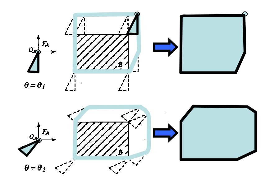
Since now the different C-space is a function of angle, we can visualize it by treating $\theta$ as a vertical axis and stacking the C-spaces:
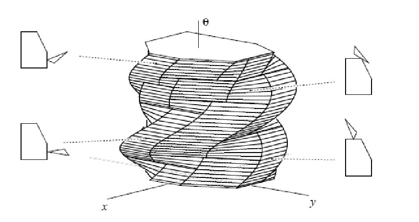
notice that already for a 2D robot with rotation, the C-space is 3D and quite complex!
C-Space with Manipulators
What about non-convex objects, such as using a manipulator? (obstacle is shown in blue)
| Manipulator | C-space |
|---|---|
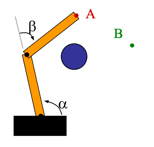 |
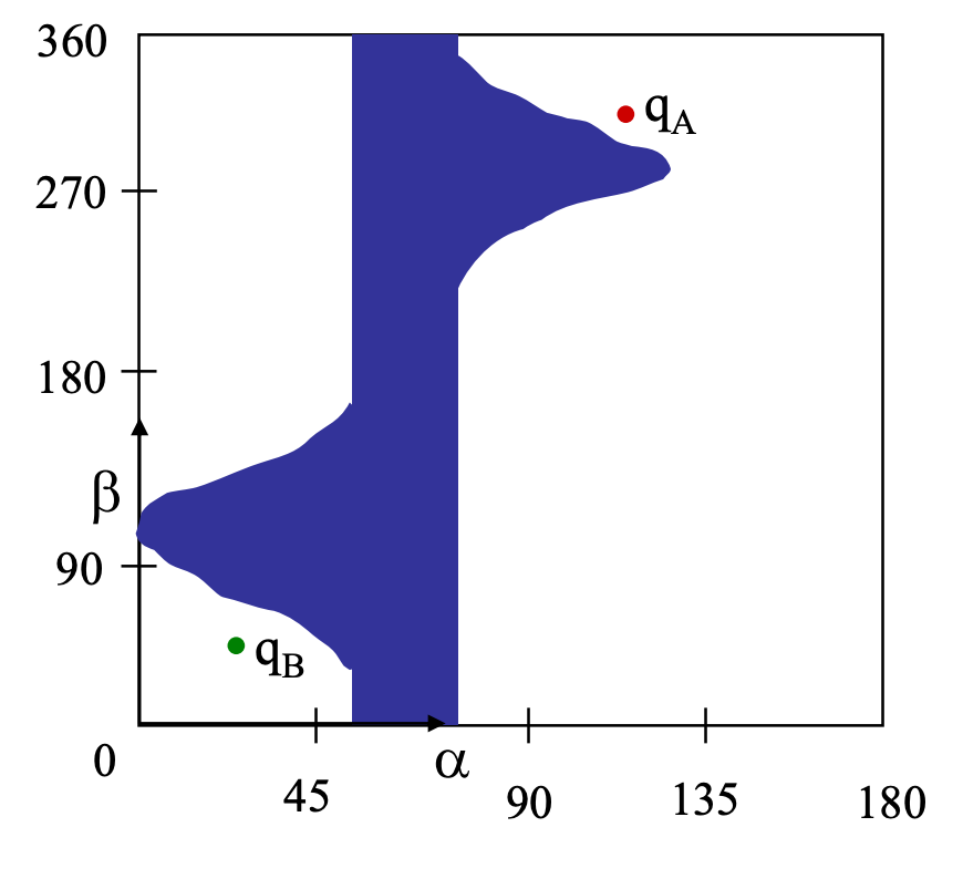 |
It turns out this is extremly complicated, and currently we are still mainly using sampling based approaches. Note that:
- the C-space is paramterized only by two variables $\alpha$ and $\beta$. So its dimension is a torus $=\mathbb{S}\times\mathbb{S}$
- visually it makes sense: only if $\alpha$ is large (e.g., $\ge 135 \degree$) the angle $\beta$ can rotate freely
Kinematics
Given a C-space and some points on it, how to do mathematically map it back to the real robot (i.e., workspace). For example, given the two angles, compute what the manipulator will actually look like.
A robot’s kinematics is a mapping from its C-space to its workspace.
In this section, we will mostly focus on (fixed base) manipulators.
note that:
-
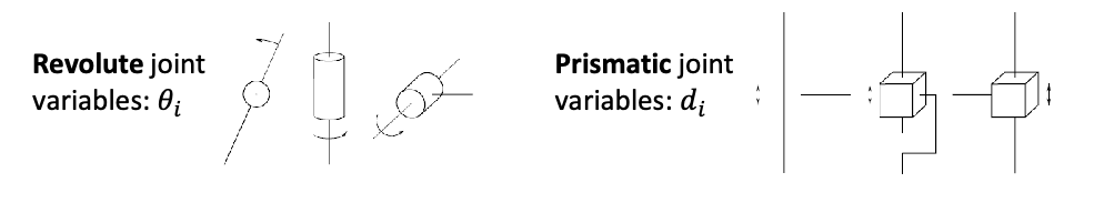
we will also assume a joint (the black dot) only has one degree of freedom. If we have $>1$, we can simply consider multiple joints and combine them.
-
often $\theta_i$ is defined relatitve to the previous link
-
there are two types of joint: a rotational and a translational one
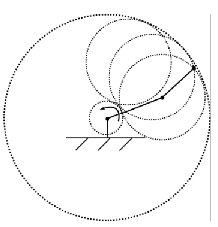
Since the useful part is the end effector, we consider the workspace of a manipulator = points reachable by the end effector
For example, a planer RR arm (revolute + revolute) covers a workspace of an annulus in $\R^2$:
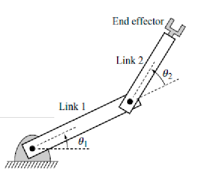
Forward Kinematics
Forward kinematics: maps from its joint variables (e.g., angles) to the world position and orientation (pose) of its links
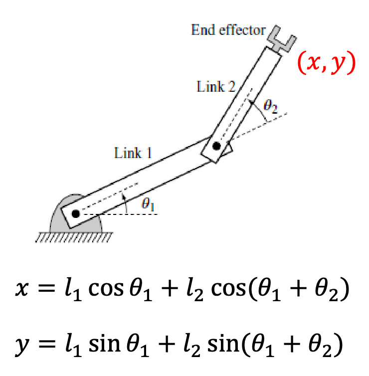
For example, given two angles, we can compute the position $(x,y)$ of the end effector:
| Visually | Mathematically |
|---|---|
 |
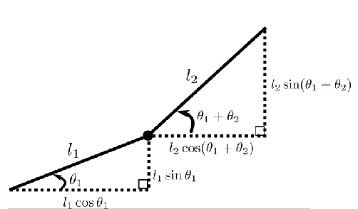 |
where here we are mainly relying on geometry, so that:
\[\begin{align*} x &= l_1 \cos\theta_2 + l_2 \cos(\theta_1 + \theta_2) \\ y &= l_1 \sin\theta_2 + l_2 \sin(\theta_1 + \theta_2) \end{align*}\]but this can quickly get very complicated. The trick is to use frame transformations matrices, where you will find that:
- the position (i.e. $(x,y,z)$) of the end effector is exactly the last column vector of the matrix
- the orientation of the end effector (i.e., if it is tilted, rotated) is found in the rotation submatrix
2D Coordinate Frames
Consider the following idea:
- label the body frames of each joints and end effector (red), and the fixed world frame as well (blue)
- then, figure out the transformation from the fixed world frame to the end effector frame
- since this transformation will tell you how to map anything from origin to the end effector, we automatically obtain the position and orientation of the end effector by reading off from the transformation matrix
Visually, we would first draw out the axes:
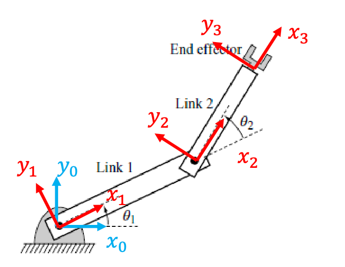
Then consider the transformations from one frame to another (which conveniently will only be a single rotation and a translation):
\[T_{i}^{i-1} = \begin{bmatrix} \cos\theta_i & -\sin\theta_i & l_{i-1} \\ \sin\theta_i & \cos\theta_i & 0 \\ 0 & 0 & 1 \end{bmatrix}\]Since each frame is drawn relative to the previous frame, we can describe the final end effector’s body frame relative to the fixed frame using:
\[T_{m+1}^0 = T_1^0 T_{2}^1 ... T^{m}_{m+1}\]and we would be able to read off the position and orientation of the end effector from $T_{m+1}^0$.
For example: consider a RRR arm, where we have three joint variables $\theta_1, \theta_2, \theta_3$ in C-space
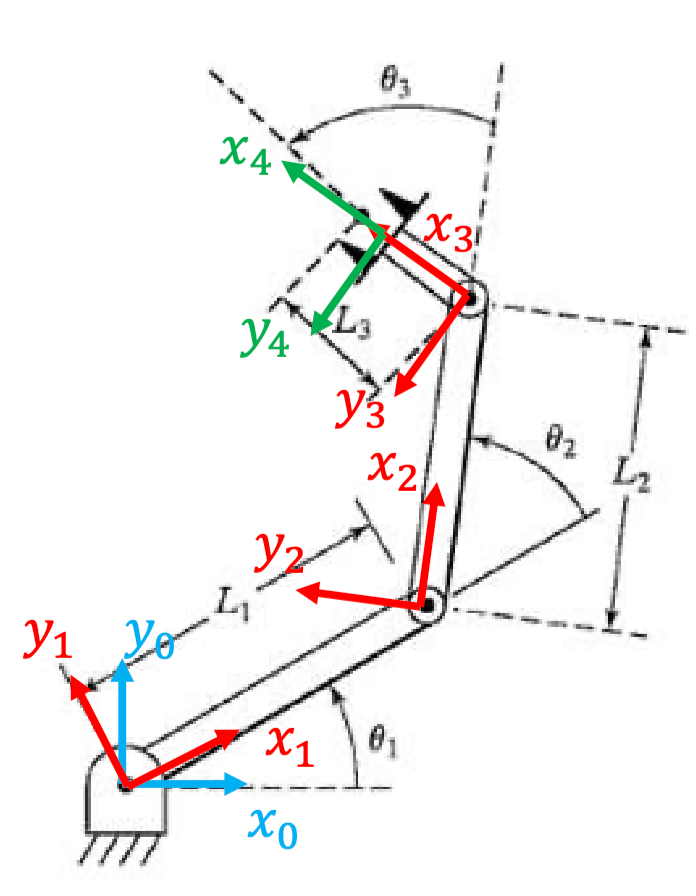
So then:
-
frame 0 to 1 we only have rotation:
\[T_1^0 = \begin{bmatrix} \cos\theta_1 & -\sin\theta_1 & 0 \\ \sin\theta_1 & \cos\theta_1 & 0 \\ 0 & 0 & 1 \end{bmatrix}\] -
frame 1 to 2 and 2 to 3, we have rotation and translation:
\[T_2^1 = \begin{bmatrix} \cos\theta_2 & -\sin\theta_2 & l_1 \\ \sin\theta_2 & \cos\theta_2 & 0 \\ 0 & 0 & 1 \end{bmatrix}, \quad T_3^2 = \begin{bmatrix} \cos\theta_3 & -\sin\theta_3 & l_2 \\ \sin\theta_3 & \cos\theta_3 & 0 \\ 0 & 0 & 1 \end{bmatrix}\] -
frame 3 and frame 4 we just have a single translation
\[T_4^3 = \begin{bmatrix} 1 & 0 & l_3 \\ 0 & 1 & 0 \\ 0 & 0 & 1 \end{bmatrix}\]
This results in
\[T_4^0 = T_1^0 T_2^1 T_3^2 T_4^3 = \begin{bmatrix} \cos(\theta_{1} + \theta_{2} + \theta_3) & -\sin(\theta_{1} + \theta_{2} + \theta_3) & l_1\cos\theta_1 + l_2\cos(\theta_1 + \theta_2) + l_3\cos(\theta_{1} + \theta_{2} + \theta_3) \\ \sin(\theta_{1} + \theta_{2} + \theta_3) & \cos(\theta_{1} + \theta_{2} + \theta_3) & l_1\sin\theta_1 + l_2\sin(\theta_1 + \theta_2) + l_3\sin(\theta_{1} + \theta_2 + \theta_3) \\ 0 & 0 & 1 \end{bmatrix}\]which we will use a shorthand notation:
\[T_4^0 = \begin{bmatrix} c_{123} & -s_{123} & l_{1} c_1 + l_{2} c_{12} + l_{3} c_{123} \\ s_{123} & c_{123} & l_{1} s_1 + l_{2} s_{12} + l_{3} s_{123} \\ 0 & 0 & 1 \end{bmatrix}\]How can we interpret this? Realize that:
-
the last column describes the position of the end effector:
\[(x,y) = (l_{1} c_1 + l_{2} c_{12} + l_{3} c_{123}, l_{1} s_1 + l_{2} s_{12} + l_{3} s_{123})\] -
the upper left matrix describes the orientation of the end effector:
\[\hat{x} = \begin{bmatrix} c_{123} \\ s_{123} \\ \end{bmatrix}, \quad \hat{y} = \begin{bmatrix} -s_{123} \\ c_{123} \\ \end{bmatrix}\]
For example: RPR arm with $(\theta_1, d_2, \theta_3)$, so we also have translations in the middle:
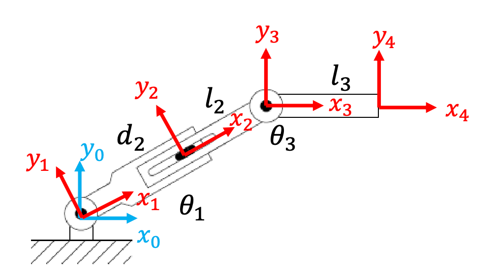
Again, after drawing the frames, we consider:
-
frame 0 to 1, we only have rotation
\[T_1^0 = \begin{bmatrix} \cos\theta_1 & -\sin\theta_1 & 0 \\ \sin\theta_1 & \cos\theta_1 & 0 \\ 0 & 0 & 1 \end{bmatrix}\] -
frame 1 to 2, we have only translation:
\[T_2^1 = \begin{bmatrix} 1 & 0 & d_2 \\ 0 & 1 & 0 \\ 0 & 0 & 1 \end{bmatrix}\] -
frame 2 to 3, we have rotation and translation:
\[T_3^2 = \begin{bmatrix} \cos\theta_3 & -\sin\theta_3 & l_2 \\ \sin\theta_3 & \cos\theta_3 & 0 \\ 0 & 0 & 1 \end{bmatrix}\] -
frame 3 to 4, we have only translation:
\[T_4^3 = \begin{bmatrix} 1 & 0 & l_3 \\ 0 & 1 & 0 \\ 0 & 0 & 1 \end{bmatrix}\]Hence altogether we have:
where again, we can read of the actual position and orientation of the end effector from this matrix.
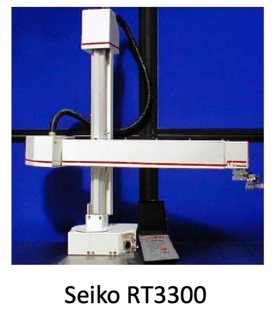
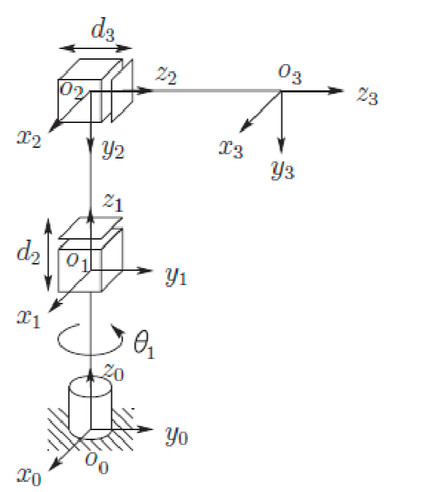
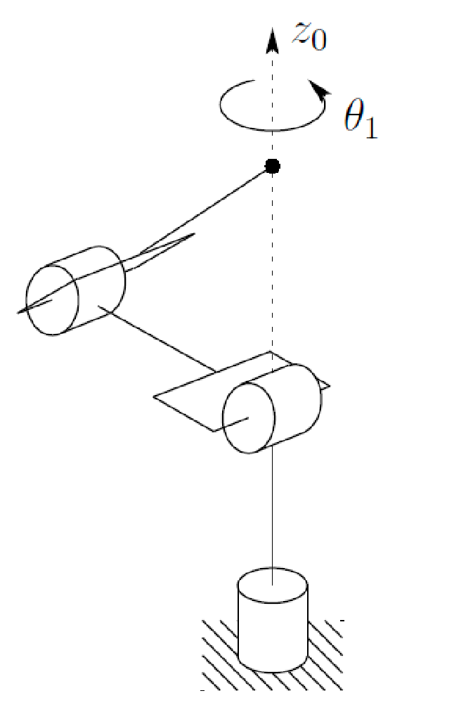
Cylindrical Arm
Now here is a more complicated manipulator that can rotate along $z$-axis:
| Cylindrical Manipulator | Annotated Body Frames |
|---|---|
 |
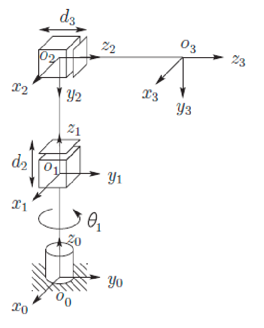 |
So how do we obtain the position and orientation of the end effector?
- frame 0 to 1 can rotate and move up and down. Specifically, we rotated $\theta_1$ by axis $z_0$, and translated along $z_0$ by $d_1$
- frame 1 to 2 can also rotate and move. Specifically, we rotated $- \pi / 2$ about axis $x_1$, and translated along $z_1$ by $d_2$
- frame 2 to 3 is the end effector, which translates along $z_2$ by $d_3$
This results in:
\[T_3^0 = \begin{bmatrix} c_1 & 0 & -s_1 & -s_1 d_3 \\ s_1 & 0 & c_1 & c_1 d_3 \\ 0 & -1 & 0 & d_1 + d_2 \\ 0 & 0 & 0 & 1 \end{bmatrix}\]where again, the last column gives you the position of the end-effector, and orientation is given by the upper left matrix.
Inverse Kinematics
Sometimes, you also want to do the reverse: given a position/orientation of the end-effector, find the joint configurations $q$ to achieve this.
The inverse kinematics problem is much harder since the FK are nonlinear!
Why? For example:
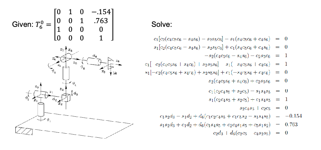
which is intrinsically because the transformation matrix is large in dimension (last row is skipped).
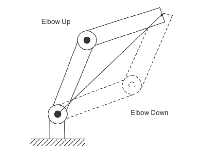
For some simple case, we can solve it algebraically. Given $(x,y)$ here, solve for $\theta_1, \theta_2$:
before we even try to solve this, notice a natural constraint:
\[(l_1-l_2)^2 \le x^2 + y^2 \le (l_1+l_2)^2\]which is this annulus region we talked about before: the end effector cannot possibly be outside that space!
If this is an allowed position, we can solve it algebraically by:
- first eliminating $\theta_1$:
- then you will already find two solutions for $\theta_2$:
- and you can solve $\theta_1$ by plugging $\theta_2$ in, and obtain:
this makes physical sense as it corresponds to:
Note: $\arctan2$ function is different from the normal $\arctan$, where you can preserve sign information (because $\arctan(y/x)=\arctan(-y/-x)$). Visually, it looks like:
this is used mainly in programming, and many libraries provide this function.

Robot Velocities
The forward kinematics tells us the pose of the end effector (i.e., position and orientation). But our robot moves around:
The time derivative of the Forward Kinematics gives the velocity of the end effector.
- effectively, it helps us to compute $(\dot{x}, \dot{y}, \dot{z})$ from joint velocities $\dot{\mathbf{q}}$.
- this velocity information is also surprisingly helpful for us to solve some inverse kinematics problems (by gradient descent)
We start with the end effectors position as a function of its configuration:
\[x(\mathbf{q}), y(\mathbf{q}), z(\mathbf{q})\]we are interested in:
\[\frac{d}{dt}(x(\mathbf{q}), y(\mathbf{q}), z(\mathbf{q}))\]using chain rules, this gives (assuming $\mathbf{q}\in \R^m$)
\[\mathbf{v} = \frac{d}{dt} \begin{bmatrix} x(\mathbf{q}) \\ y(\mathbf{q}) \\ z(\mathbf{q}) \end{bmatrix} = \begin{bmatrix} \frac{\partial x}{\partial q_1} \frac{d q_1}{dt} + ... + \frac{\partial x}{\partial q_m} \frac{d q_m}{dt} \\ \frac{\partial y}{\partial q_1} \frac{d q_1}{dt} + ... + \frac{\partial y}{\partial q_m} \frac{d q_m}{dt} \\ \frac{\partial z}{\partial q_1} \frac{d q_1}{dt} + ... + \frac{\partial z}{\partial q_m} \frac{d q_m}{dt} \end{bmatrix} = \begin{bmatrix} \frac{\partial x}{\partial q_1} & ... & \frac{\partial x}{\partial q_m} \\ \frac{\partial y}{\partial q_1} & ... & \frac{\partial y}{\partial q_m} \\ \frac{\partial z}{\partial q_1} & ... & \frac{\partial z}{\partial q_m} \end{bmatrix} \begin{bmatrix} \frac{d q_1}{dt} \\ \vdots \\ \frac{d q_m}{dt} \end{bmatrix} = J(\mathbf{q}) \dot{\mathbf{q}}\]so ultimately, velocity is some matrix (a Jacobian) times the joint velocity $\dot{\mathbf{q}}$. Later on you will also see that:
- the $i$-th column in the Jacobian is $\in \R^{3}$, which tells you the velocity direction of the end effector if you only moved that joint $q_i$
- so the velocity of the end effector is a linear function of the joint velocity $\dot{\mathbf{q}}$.
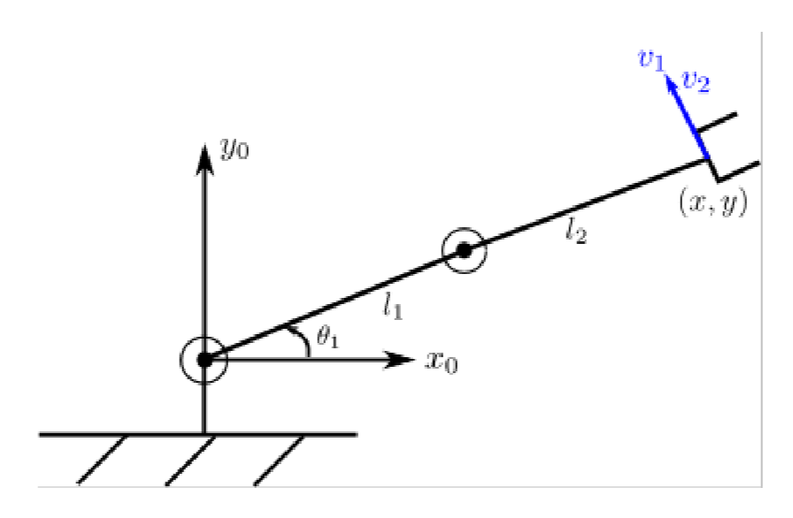
For example: in an planar RR arm we have:
\[\begin{bmatrix} \dot{x} \\ \dot{y} \end{bmatrix} = J(\theta_1, \theta_2) \begin{bmatrix} \dot{\theta_1} \\ \dot{\theta_2} \end{bmatrix}\]where the jacobian is:
\[J(\theta_1, \theta_2) = \begin{bmatrix} -l_1 \sin\theta_1 - l_2 \sin(\theta_1 + \theta_2) & -l_2 \sin(\theta_1 + \theta_2) \\ l_1 \cos\theta_1 + l_2 \cos(\theta_1 + \theta_2) & l_2 \cos(\theta_1 + \theta_2) \end{bmatrix} = \begin{bmatrix} \vec{v}_1 & \vec{v}_2 \end{bmatrix}\]where notice that column vector is perpendicular from the effector to the joint. This means the direction of the velocity if you only move that joint.
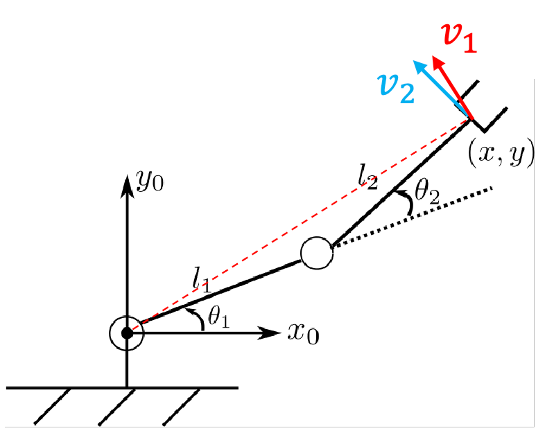
In general, this also means the column space of $J$ is the set of all possible end effector velocities.
Singular Configurations
Typically, if your work space is $\R^n$, then your Jacobian could have $n$ independent columns (e.g., typically $n=3$).
Recall:
- the rank of a matrix is the number of linearly independent columns.
- the null space of a matrix $A$ is the set of all vectors $x$ such that $Ax=0$.
- if A has a non-trivial nullspace, it is not invertible and thus $\det A = 0$.
It is possible for $J$ to have rank $< n$ due to some special structure of the robot. If this happens, its called singular configurations.
- this means that there is some direction you cannot move the end effector, even if you moved all the joints.
- if $J$ is square, this also means it is non-invertible (also called being “singular”)
- finally, since its no longer full rank, there is a non-trivial null space of $J$ = there will be certain non-zero joint velocities such that the end effector does not move.
For example, if for some reason your $\theta_2=0$ is “stuck” and cant move for a while:
then our Jacobian is
\[J(\theta_1, 0) = \begin{bmatrix} -l_2 \sin\theta_1 - l_2 \sin\theta_1 & -l_2 \sin\theta_1 \\ l_1 \cos\theta_1 + l_2 \cos\theta_1 & l_2 \cos\theta_1 \end{bmatrix}\]Then notice that this has a null space:
\[\text{Null}(J(\theta_1, 0)) = \text{Span}(-l_2, l_1+l_2)\]this means even if you moved the joints:
\[\begin{bmatrix} \dot{\theta_1} \\ \dot{\theta_2} \end{bmatrix} = \alpha \begin{bmatrix} -l_2 \\ l_1+l_2 \end{bmatrix}\]the end effector will not move.
For example: consider a cylindrical arm $\mathbf{q}=(\theta_1, d_2, d_3)$
| Visual | Jacobian |
|---|---|
 |
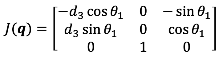 |
first some sanity checks:
-
the only way to give $z_0$ movement is in the second column, which corresponds to moving $d_2$ = makes sense!
-
to find singular configurations, we can solve for the nullspace or simply notice that $\det J = 0$. This gives us:
\[0 = \det J = -d_3 \cos^2 \theta_1 - d_3 \sin^2 \theta_1 = -d_3\]so if $d_3 = 0$, we will have a non-trival null space = singular configuration. In fact, if $d_3=0$, the end effector will lie on the $z_0$ axis, and actuating $\theta_1$ produces no linear velocity
For example: consider an anthropomorphic manipulator with $\theta_1, \theta_2, \theta_3$:
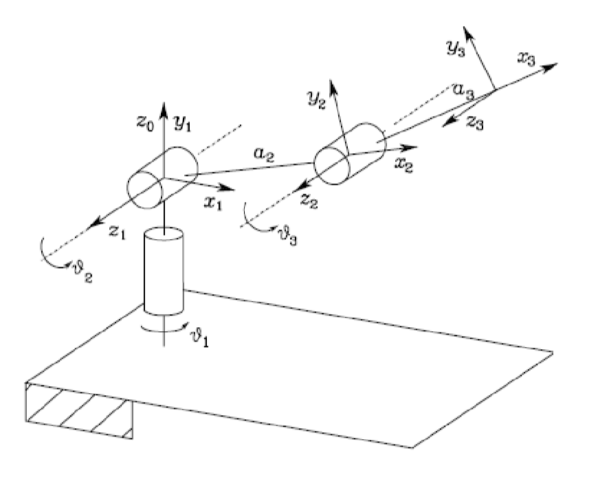
where if you look at the singular configurations, set $\det J = 0$ and you wil find:
\[0 = \det J = a_2a_3 \sin\theta_{3} \cdot (a_{2} \cos\theta_{2} + a_{3} \cos\theta_{2}\cos\theta_{3})\]-
so consider $\sin \theta_3 = 0$. This meaning multiples of $\pi$ gives you singular configurations = corresponding to your third joint being parallel to the second joint
-
or $a_2\cos\theta_2 + a_3 \cos\theta_2\cos\theta_3 = 0$. This corresponds to
again, the end effector has no linear velocity (its rotating, but not moving) if we move $\theta_1$
Numerical Inverse Kinematics
Using a numerical approach to solve the Inverse Kinematics problem.
- a counterpart of our algebraic solutions in Inverse Kinematics
- drawback: can suffere from numerical instabilities, and require more computation
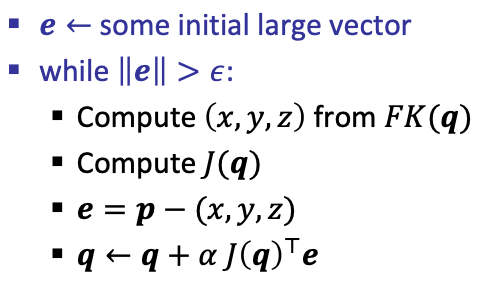
Idea: suppose we want the end effector to be at position $(x^, y^, z^*)$, we can define an error function given its current position:
\[MSE = \frac{1}{2}((x^*-x)^2 +(y^*-y)^2 + (z^*-z)^2)\]so our goal is simply to numerically find the $\mathbf{q}$ such that:
\[\min_{\mathbf{q}} \frac{1}{2}((x^*-x)^2 +(y^*-y)^2 + (z^*-z)^2) = \min_{\mathbf{q}} \mathcal{L}\]so how do we find such $\mathbf{q}$ given this loss function? Gradient descent, which just takes a step using the partial derivatives
\[\frac{\partial \mathcal{L}}{\partial \mathbf{q}} = \left [\frac{\partial \mathcal{L}}{\partial q_1}, \frac{\partial \mathcal{L}}{\partial q_2}, ..., \frac{\partial \mathcal{L}}{\partial q_m} \right ]\]and we update:
\[\mathbf{q} \gets \mathbf{q} -\frac{\partial \mathcal{L}}{\partial \mathbf{q}}\]until convergence. But it turns out that we can write this gradient in another format that relates to what we discussed before:
\[\begin{align*} \frac{\partial \mathcal{L}}{\partial \mathbf{q}} &= (-x^* - x(\mathbf{q})) \frac{\partial x }{\partial \mathbf{q}} - (y^* - y(\mathbf{q})) \frac{\partial y }{\partial \mathbf{q}} - (z^* - z(\mathbf{q})) \frac{\partial z }{\partial \mathbf{q}} \\ &= - \begin{bmatrix} \frac{\partial x}{\partial \mathbf{q}} & \frac{\partial y}{\partial \mathbf{q}} & \frac{\partial z}{\partial \mathbf{q}} \end{bmatrix} \begin{bmatrix} x^* - x(\mathbf{q}) \\ y^* - y(\mathbf{q}) \\ z^* - z(\mathbf{q}) \end{bmatrix} \\ &= -J(\mathbf{q})^T e(\mathbf{q}) \end{align*}\]so the gradient is just a negative Jacobian transpose times error vector! This again makes sense, since we just want to move in the direction to change $x,y,z$!
For example: given some initial configuration $\mathbf{q}$, desired position $\mathbf{p}$, step size $\alpha$, and an error threshold $\epsilon$:
Since this only uses first order gradient, we can get local minima when $J(\mathbf{q})^T e(\mathbf{q})=0$. This means that:
- $e(\mathbf{q})$ is in the null space of $J(\mathbf{q})^T$.
-
Given a target position $(x^, y^, z^*)$, the entire thing is a function of $\mathbf{q}$. This means if you get into that $\mathbf{q}$ gradient descent will be stuck there
- This has a physical interpretation: these are the singular configurations!
For example, we knew that $\theta_2$ fixed at $\theta_2=0$ gives a singular configuration. Then if we consider doing gradient descent at this configuration:
\[J^{T}(\theta_1, 0) = \begin{bmatrix} -(l_{1} + l_2) \sin \theta_{1} & (l_{1} + l_2) \cos\theta_{1} \\ -l_2 \sin\theta_{1} & l_2 \cos\theta_{1} \end{bmatrix}\]Then if, given some target position $(x^, y^)$, we ended up with:
\[e(\mathbf{q}) = \beta \begin{bmatrix} \cos\theta_1 \\ \sin\theta_1 \end{bmatrix}\]gradient descent will stop, and we are stuck. This visually corresponds to the case when:
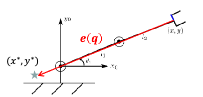
then given the star is your target position, but moving the joints in any direction away from $\theta_1, 0$ will increase the error function. So you are now stuck in a local minima.
Search-Based Planning
Given a robot and a world $\mathcal{W}$, we want to move the robot from one place to another without colliding.
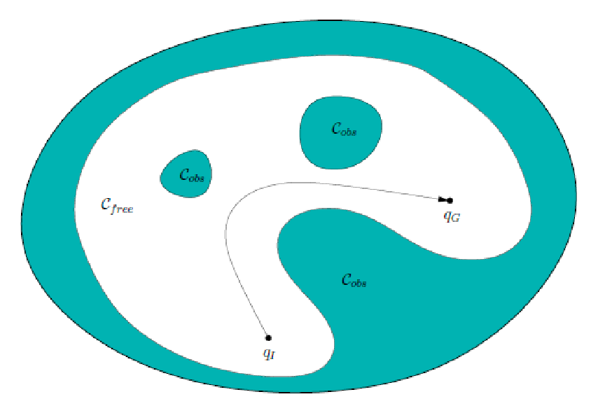
Motion Plannning: find a path in configuration space $c: [0,1] \to Q_{\mathrm{free}}$ such that:
\[c(0) = q_1, \quad c(1) = q_G\]or report if no such path exists.
- so we are given initial and goal configuration $q_1$, $q_G$, and we want to find a path
- a path in the configuration space can then be easily translated to a path in the workspace -> physically move!
Visually:
There are many algorithms that can do this, and a good algorithm should satisfy:
- Completeness: Guarantee of finding a solution or reporting failure
- Optimality: Path length, execution time, energy consumption of the robot, etc.
- Efficiency: Algorithm runtime and memory complexity. This would also relate to C-space size; worst vs average case
- Offline vs online: does planning occur in real-time, using sensor information?
Types of algorithms
- Search-based: discrete C-space into graphs or grids, and then do planning
- Combinatorial: plan using the full C-space by exploiting some geometry properties of the environment
- Sampling -based: sample C-space to construct discrete representations
both Search and Combinatorial methods yield completeness and optimality guarantees, but become expensive in high-dimensional space. Sampling-based methods are very efficient even in high-dimensional C-space, but weaker in completeness and optimality.
Grids and Obstacles
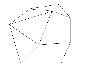
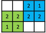
Assuming we konw the full C-space already, and that its almost euclidean, we can discretize the C-space (given some resolution hyperparameter)
| Original | Discretized |
|---|---|
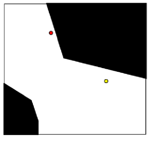 |
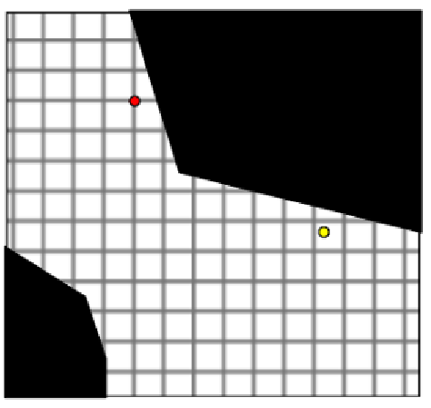 |
Then we can consider any cell that (partially) contain the obstacle to be out of bounds.
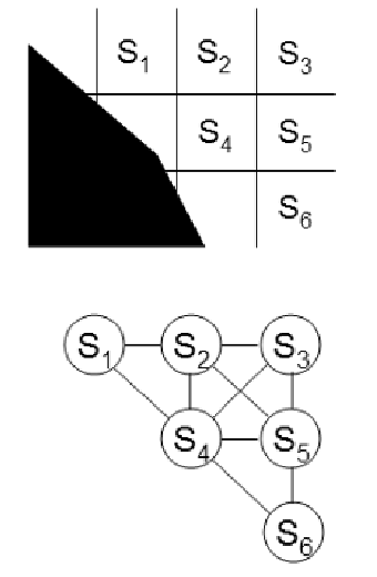
For search-based algorithms in this section, we first discretize them into grid, then convert the grids into graphs, and finally do planning on the graph.
So we will almost always be working on the graph below (for this section)
note that here we have a couple of “hyperparameters” to consider:
- resolution of the grid (i.e., how many cells per unit)
- grid connectivity
- use 4-point connectivity: robot only goes up, down, left, right
- use 8-point connectivity: The above, plus 4 diagonals
if we use high resolution + high connectivity, it could make the graph denser = more runtime to plan.
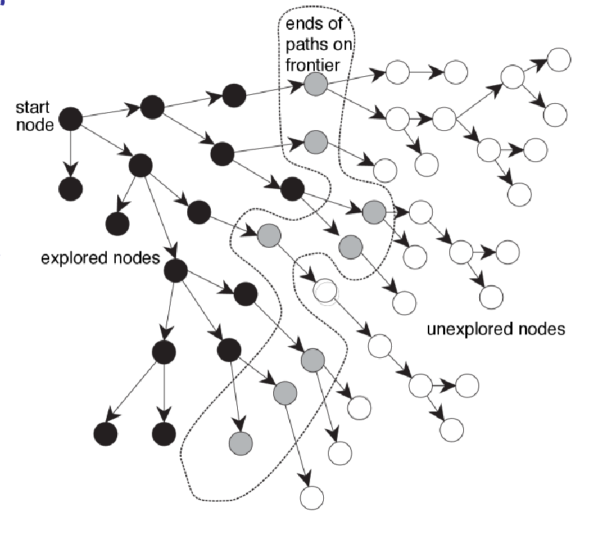
Search Trees
Search algorithms in this section then typically follow the template:
- traverses from the initial state and iteratively visit un-explored nodes
- mark visited nodes as explored
- (different in different algorithms) consider which node to visit next
For all algorithms in this section, assume we know the entire region of interest. So then planning is done entirely offline without any interaction with the environment.
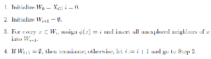
Therefore, most search-based algorithms look like:
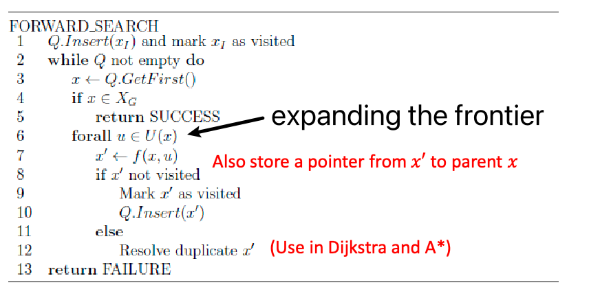
where:
- $U(x)$ means all the transitions you can have at node $x$, i.e., edge to children nodes
- $f(x,u)$ gives you the next state/node
- the $\text{resolve duplicate }x’$ means we might update some statistics about the graph or $x’$.
- difference between different search algorithms would come in $x \gets \text{Q.GetFirst()}$ and $\text{resolve duplicate }x’$
DFS and BFS
Both are very similar, with the mainly differ in $x \gets \text{Q.GetFirst()}$:
Depth first search: expand the deepest state we have in $Q$ so far.
- not guaranteed to find a solution if state space is infinite
- not guaranteed to find shallowest or cheapest solution
- but its space complexity is usually lower than other algorithms
Breadth first search: expand the shallowest state we have in $Q$ so far (i.e., check each level of the tree before the next)
- guaranteed to return a shallowest solution, though it is not necessarily the lowest cost since each edge can have different costs
- typically much more memory-intensive than DFS
Dijkstra’s Algorithm
We can generalize BFS with edge costs. This is basically Dijkstra’s algorithm.
Dijkstra: nodes in $Q$ are ordered by increasing values of cumulative cost from start node, i.e., check lowest cost node first! Essentially
- Priority function in 𝑄 is the cumulative cost of a state from initial
- Expanding the frontier = visit a new node and adding transition cost to parent cost
Guaranteed to be optimal if there exists a finite cost path to reach $G$.
But note that:
- To guarantee cost optimality, we must keep track of path costs
- It may not terminate (you can adversarially construct a graph to make this happen), but if cost is finite it will terminate.
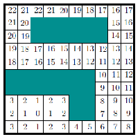
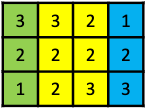
Navigation Functions
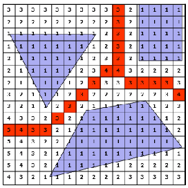
If your edges are bi-directional and cost is the same for either direction, you can use Dijkstra to obtain “value functions” that looks like this:
| Optimal Value Function | Optimal Policy |
|---|---|
 |
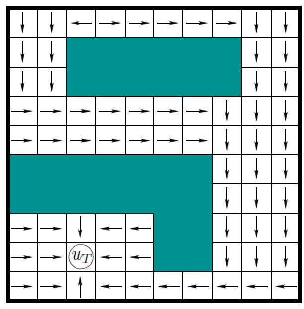 |
How? Simply:
- run Dijkstra starting from goal ($u_T$), terminate until all states visited
- now we have lowest costs from every state to a goal!
This optimal value function is also called a navigation function $\phi$ in robotics:
\[\phi: \mathcal{Q} \to \R\]then given the *optimal value function $V^(s)$*, we can easily extract the optimal policy $\pi^$ for each node/state.
Wavefront Algorithm
If all edges have a cost of 1, we can modify BFS to obtain the same optimal value function by imaging waves:
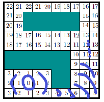
where we basically consider all elements expanded and labeled identically in each iteration.
If we want, we could also modify this to work with non-uniform costs, but then it would be more like Dijkstra’s algorithm.
Heuristics Functions
Since robotics has a lot to do with real-world scenarios, we often have heuristics: what is very likely a bad next state to explore. Specifically, we will see that (good) heuristics function can speed up algorithms significantly.
Heuristic function $h(x)$: Estimated cost of cheapest path from $x$ to a goal state. An example would be euclidean distance.
A heuristic $h$ is admissable if $h(x) \le h^(x)$ where $h^(x)$ is the true cost from $x$ to goal.
- An example would again be using euclidean distance above
- very useful property = can guarantee A* search to return optimal solutions
Interestingly, if you consider grid navigation with all transitions have cost $1$:
- if we have 4 point connectivitiy in this graph, then using both $L^1$ distance of $L^2$ distance are admissible heursitics
- if we have 8 point connectivity, then we need a $1/\sqrt{2}$ factor for $L^2$ distance to be admissible.
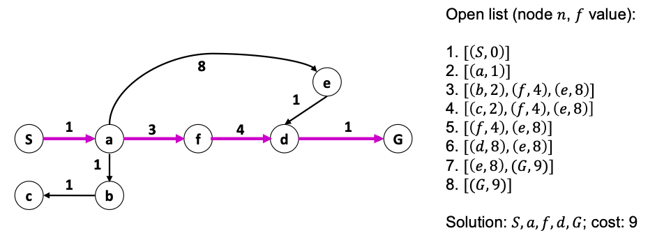
A* Search
*$A^{}$ search*: modify Dijkstra to evaluate each node based *on both cumulative cost and heuristic value, so that Dijkstra’s cost function is now:
\[f(n) = \mathrm{cost}(n)+ h(n)\]such that nodes in the frontier $Q$ is sorted based on the modified cost $f$.
But why does it matter? This is often more efficient than Dijkstra, as heuristic can “steer” the search to investigate more promising areas of the search space.
For example:
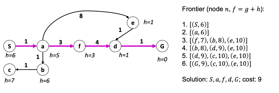
where you see that the heuristics are pushing us away from trying non-promising area early.
Weighted A* Search
With robotics and real-time planning, time efficiency is often more important than optimality.
Weighted $A^{*}$ Search: put a weight on the heuristics cost:
\[f (n) = \mathrm{cost}(n) + \alpha h(n)\]where this gives us:
- greedy best-first if $\alpha \to \infty$
- if $\alpha = 1$ we get A* search, and if $\alpha = 0$ we get Dijkstra algorithm
You can tune this $\alpha$ to expand less nodes to pop the goal out of the stack = faster.
However, the final solution may not be optimal: If optimal solution has cost $C^$, weighted A solution may cost up to $\alpha C^*$.
Dynamic Replanning
What if our C-space changes over time?
- Costs or transitions may change after making a plan
- Robot may discover new information while executing a plan
Note that the algorithms introduced before in Search-Based Planning do offline planning. Obviously you could just re-run the whole thing, but ths is very inefficient (e.g., changes are small). Can we reuse prior computations to make this more efficient?
A* with Label Correction
One approach is to modify A* to keep track of previous results, and only recompute/expand some nodes when there are some inconsistencies between what I had before and what I have now.
$A^{*}$ with label correction: for each node $n$, we store:
- the actual lowest cost $g(n)=\mathrm{cost}(n)$ to traverse from start to node $n$
- another value $v(n)$ to represent the previous value of $g(n)$ = value of $g(n)$ when $n$ was most recently expanded (use $\infty$ if no history)
Then its basically the same as A* search, but we will only look into a node if $v(n) \neq g(n)$.
This means that:
- if you are running A* with label correction for the first time, everything is inconsistent, so it is equivalent to A* search
- if something changed and you run A* with label correction again, you will only recompute the nodes that are inconsistent (and the nodes affected by it).
This is achieved by the invariant:
At any given time, our frontier $Q$ only contains inconsistent nodes to explore/expand next.
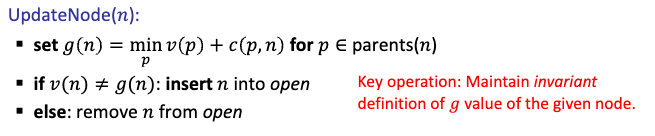
And the algorithms looks like:
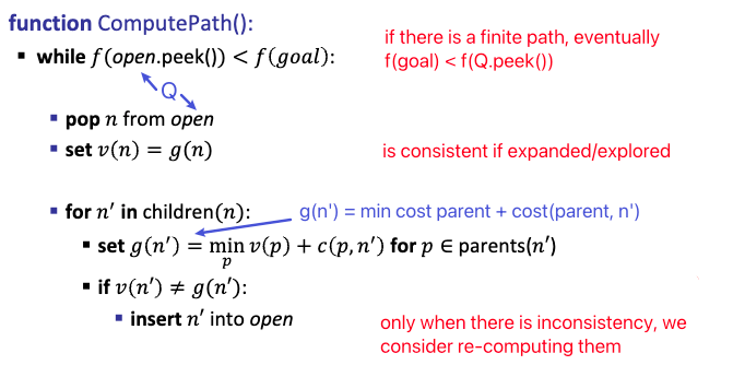
And once done, we store the computed $g,v$ values so that next time we can directly re-use them.
Note that the complicated “$g(n’)$ = min cost parent …” is to deal with the case that a node $n’$ might have multiple parent = to compute the actual shortest path to $n’$ we pick the cheapest parent.
Let’s consider an example. Suppose we are in a fresh run and we have jsut expanded $S_2, S_1$. Since $S_2, S_1$ are just expanded, they are consistent, but not the other ones:
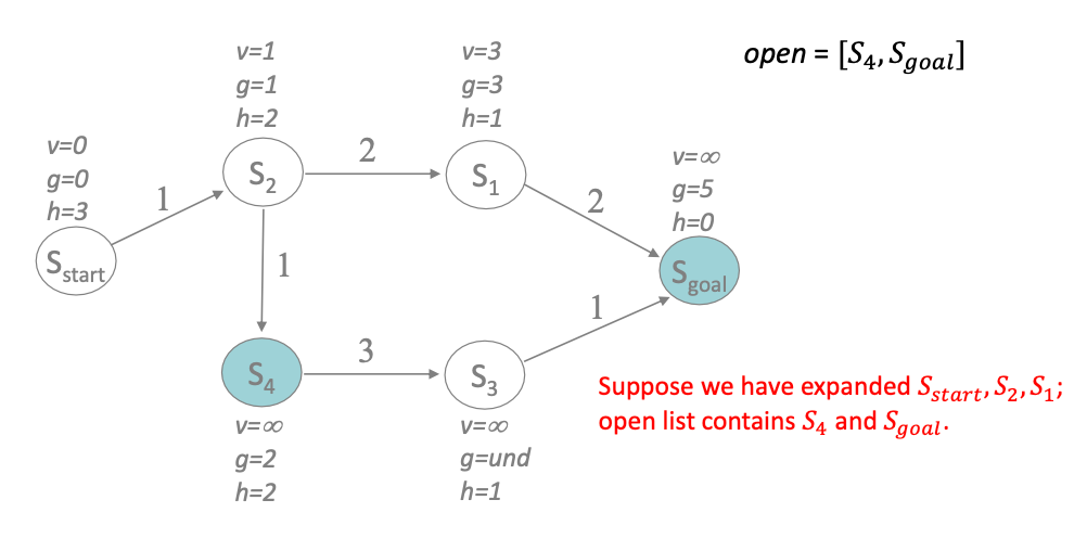
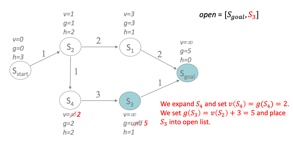
We then check $S_4$ and do:
- mark it as consistent by setting $v(S_4) = g(S_4)$
- for each of $S_4$’s next state $n’$ = only $[S_3]$ in this case
- set $\mathrm{cost}(n’) =$ cheapest parent cost + transition cost
- hence we set $g(S_3) = 2+3=5$
- check consistency $g(S_3) \overset{?}{=} v(S_3)$, and insert into open list if inconsistent
- sort the open list $Q$ by $f(n) = \min{ g(n),v(n) } + h(n)$
Next, we repeat with the goal state being the first on the priority queue:
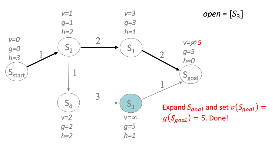
Then we are done because $f(\text{Q.peek()}) > f(S_{\mathrm{goal}})$. But before we quit:
- return the path found
- but also store all the statistics $g,v$ in memory
So when changes in the environment happens, we still re-compute from $S_{\mathrm{start}}$ but we only need to recompute nodes when we find inconsistencies.
Lifelong Planning A*
To make the A* with label correction fully correct, it turns out we need to be slightly more careful. When there are changes in the environment, and we are inspecting node $n$, we may find:
- the actual cost $g(n)$ is lower than the previous value $v(n)$ = overconsistent
- or the actual cost $g(n)$ is higher than the previous value $v(n)$ = underconsistent
To be still optimal, we need to:
- if we are overconsistent, we can repeat the same thing as A* with label correction by setting $v(n) = g(n)$ and recompute all children nodes
- if we are underconsistent, we need to recompute $v(n)$ *and* all children nodes
- and lastly, we need to consider a new end condition: we also require $v(goal) = g(goal)$ to terminate
Algorithm
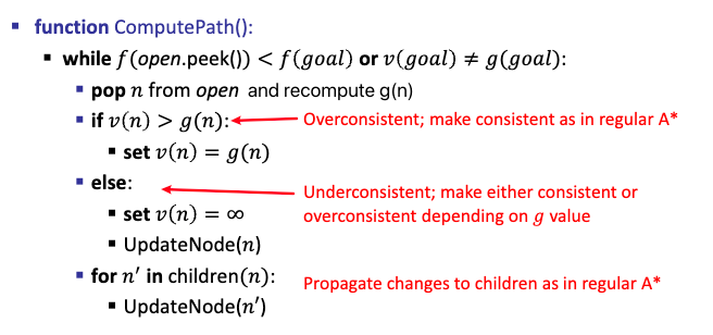
and
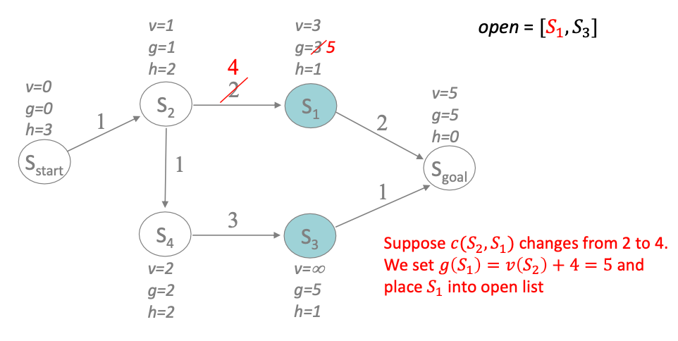
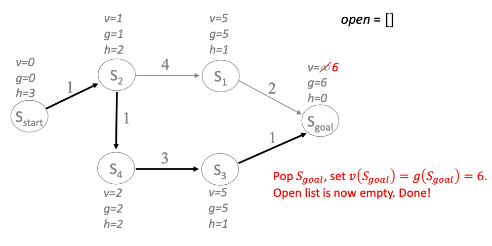
As an example, lets start off from our last example
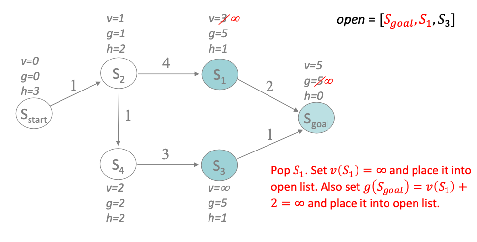
and suppose we changed an edge cost after our previous (stored) computation. If we run LSA* from $S_{\mathrm{start}}$, we will find our first inconsistency at $S_1$:
- $v(S_1)=3$ was our previously computed cost
- recomputing $g(n)$ the actual cost, we get $g(S_1)=5$
- since the actual cost is higher, we are underconsistent and we need to recompute $v(S_1)$ and all children nodes
- set $v(S_1)=\infty$ and placed back to the queue
- (
updateNode) check its children nodes, in this case $S_{\mathrm{goal}}$. It is again underconsistent, so $g \gets \infty$
| Step 1 to 2 | Step 3-5 |
|---|---|
 |
 |
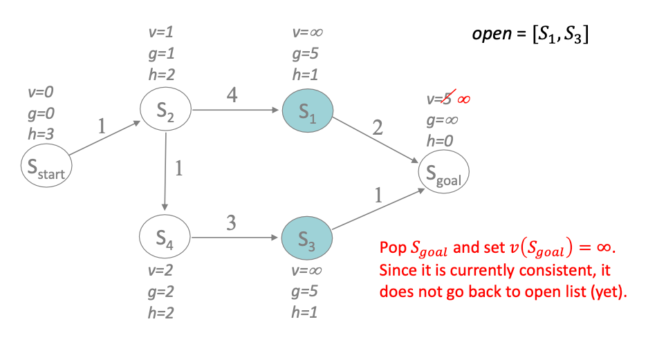
Now we expand $S_{\mathrm{goal}}$ and check if it is inconsistent. It is since $g$ was modified and became underconsistent, we need to compute $v(S_{\mathrm{goal}})$ and all children nodes again:
Next
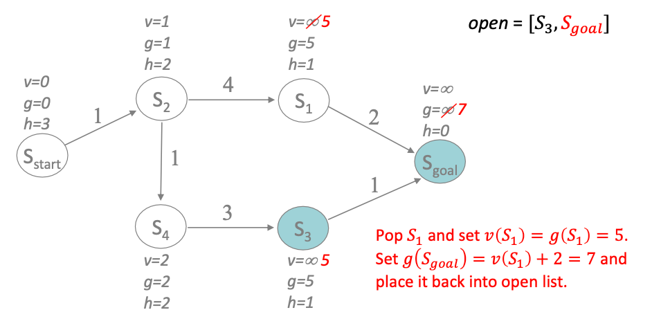
since $S_3$ is now over-consistent, we simply make it consistent and proceed
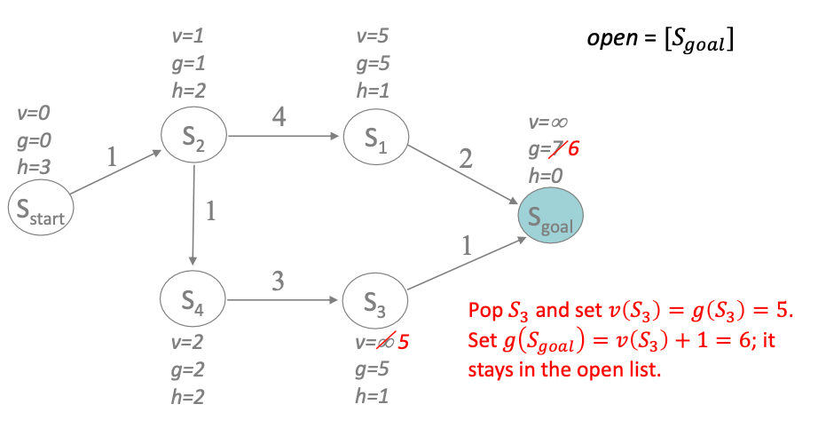
Finally we have a consistent $S_{\mathrm{goal}}$ and we terminate
As you may have noticed in this example:
- whenever a node has underconsistency, we propagate $g \gets \infty$ for its children in a “DFS” like manner
- LPA* guarantees expanded nodes have non-decreasing $f$ values over time to achieve optimality
- under-consistent nodes are expanded at most twice in LPA*
- we are only re-computing if needed
D* Lite
LPA* is still offline = we compute everything in our head when given the environment.
What if we want to execute while we are performing computation? (e.g., this may be useful when your robot does not have access to the full environment, but only what it sees right now)
Dynamic A* Lite (K&L 2002): Similar to LPA* but
- we change start node to current node whenever we replan
- we run “backwards”: instead of searching from start state, search from goal state (which doesn’t change given the above condition)
This is actually used in robotic systems, where we:
- parse what our robot see
- run D* Lite (continuously) to find some actions to do and execute
- repeat
Combinatorial Motion Planning
Last section we considered path search with graph search algorithms: 1) converting the world into a grid 2) convert the grid to a graph, and 3) do graph search.
Here we still use graph search algorithms, but we consider approaches to directly model the C-space as a graph. How do we do this?
In many motion planning problems, we can plan directly in the C-space by exploiting geometric properties and representation. Often by:
- limiting to special cases (e.g., 2D space), and assuming polygonal obstacles
- if the above holds, solutions are exact (c.f. grid approach) and complete
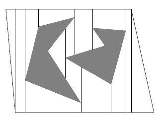
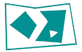
As we will focus on 2D euclidean space, polygonal obstacle regions, here is an example:
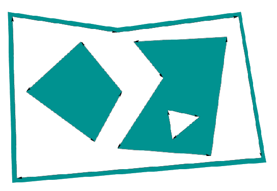
where we know the set of vertices of the obstacles. So we represent the C-space with:
- a set of half-edges, i.e., defined by pairs of vertices
- Half-edges are oriented to run counterclockwise around an obstacle
- holes in obstacles are ordered clockwise around holes
- the non-obstacle region is the empty space we want to plan on
Roadmaps
We can efficiently represent obstacle regions, but what about the free space (not using the grid approach)? What do we even want from such a representation?
We essentialy want a graph $\mathcal{G}$ that satisfies the following property:
- each vertex of $\mathcal{G}$ correspond to a point in $\mathcal{Q}_{\mathrm{free}}$
- each edge of $\mathcal{G}$ correspond to a continous path in $\mathcal{Q}_{\mathrm{free}}$
As long we have these properties, graph search algorithms can be used to find a path in $\mathcal{Q}_{\mathrm{free}}$
Furthermore:
Swath: the set of points $\mathcal{S} \subset Q_{\mathrm{free}}$ reachable by some $\mathcal{G}$ you constructed.
which is essentially a subspace of $\mathcal{Q}_{\mathrm{free}}$ that is considered by the graph. In this formulation, your graph doesn’t need to reach all points, but:
Roadmaps: a graph $\mathcal{G}$ that satisfies the above property but is also:
- accessible: there exists a path from any point in $q \in \mathcal{Q}_{\mathrm{free}}$ to some $s \in \mathcal{S}$
- connected: if there exists a path $q_{1} \to q_{2} \in Q_{\mathrm{free}}$, a path $q_1\to s_{1} \in S$, and a path $q_{2} \to s_{2} \in S$, then your roadmap should have a path $s_1 \to s_2$
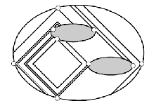
Although the above seem to be less powerful in that it does not cover all space in $\mathcal{Q}_{\mathrm{free}}$, but it can happen in practice, for example:
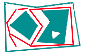
where the red edges are the road map $\mathcal{G}$:
- given any two points in the free space (except for the hole)
- you can go from one point on to the “red highway”, and then to the other point
And depending on if you just want “some path” or “the optimal path”, you can have different roadmaps.
Cell Decomposition
But how do we build such a roadmap?
One way here is to decompose free space into a union of cells, where cells are convex polygons instead of grids
- why convex polygons? If we have a convex polygon of free space, getting from any point to any other point is a simple straight line
- then, path finding becomes: find the best sequence of polygons to go through $\to$ travel within the polygons are straight lines
Note that the grid approach can be also seen as a cell decomposition:
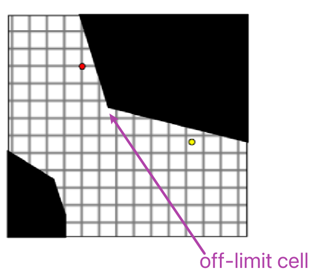
except that it does not exploit any information about the environment: in practice we need to remove those “off-limit” cells as long as there is partial collision.
So the real limitation we are trying to resolve is that:
Any grid search algorithm is only resolution-complete (I can come up with a very bad resolution where grid search will fail). Here we want to return a path as long as its feasible (irrespective of resolution)
Vertical Decomposition
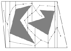
Assuming the obstacles are polygonal, we can obtain convex polygon cells by drawing lines from each obstacle vertex:
Vertical cell decomposition: partitions free space into trapezoids (2-cells) and segments/lines (1-cells)
- construct by extending a segment upward and downward from every vertex until hitting $\mathcal{Q}_{\mathrm{obs}}$
- we end up with 2-dimensional cell (trapezoid) and 1-dimensional cell (the segment/line we drew)
Then we can construct a roadmap by considering the
- consider the centroid of each cell (both 2-cell and 1-cell) as a vertex
- add an edge from each 2-cell vertex to its border 1-cell vertices
How do we use this roadmap? Consider finding a feasible path from the red cross to the red square:
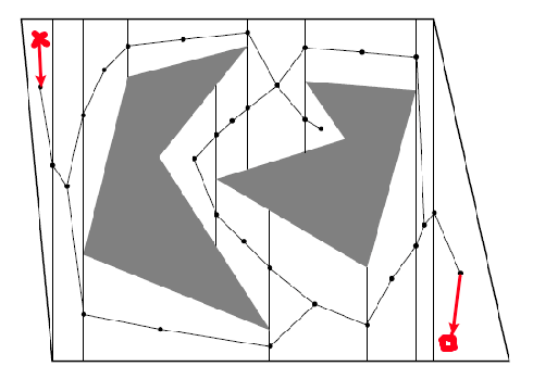
- find one way to get onto the “highway” from the red cross
- then find a way to get off the “highway” to the red square
Line Sweep Algorithm
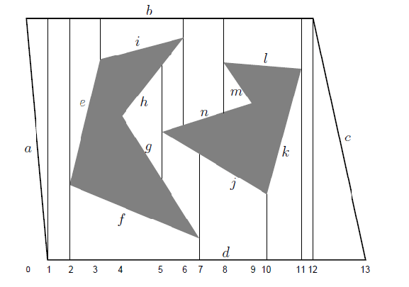
Here we describe how to obtain the vertical decomposition:
Line Sweep Algorithm imagining sweeping an infinite vertical line from left to right, but only focusing our attention when we are at obstacle vertices:
- initialization: index all obstacle edges (e.g., 0,1,2,3, …)
- sort all obstacle vertices with increasing $x$-coordinate
- for each vertex: consider an infinite line and record where it hit the obstacle and record in $L$
- make sure $L$ is sorted by index of intersected edges (to improve efficiency)
Visually:
| Grpah | Algorithm |
|---|---|
 |
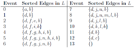 |
To be more exact, an efficient implementation of the algorithm needs to return us the trapezoidal regions at the end of the sweep. As a result, we need to consider the following cases:
- when at a vertex $v$ which has edge on both left and right of the line/segment $c$ we are sweeping:
 then the algorithm
- has the left edge $e$ is already in $L$
- remove $e$ and append $e’$
- add $c,e’,e’’$ and the next 1-cell to the trapezoidal region list
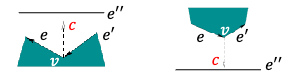
- has both edges on the left of the line/segment:
 then the algorithm:
- remove $e,e’$ from the list (using $v$’s y-coordinate to locate them quickly in $L$, which is sorted)
- if obstacle is left of $v$, add one new trapezoidal region bounded by both $c$ and $c’$
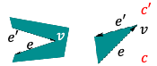
- when both obstacle edges are on the right of the line/segment
 then the algorithm:
- add both edges to the list
- if obstacle is right of $v$, add two new trapezoidal regions bounded by $c$ and $c’$
note that since the intersected edges is sorted, finding the edge takes only $O(\log n)$ time (e.g., binary search). Since we then sort and process each vertex once, the total time is $O(n \log n)$.
Adjacency Graph and Path Finding
In summary, to do path finding you can:
- do vertical decomposition
- construct a roadmap ($\mathcal{G}$) using centroids of the cells
- connect your start and end point to the roadmap
- run a graph search algorithm on $\mathcal{G}$
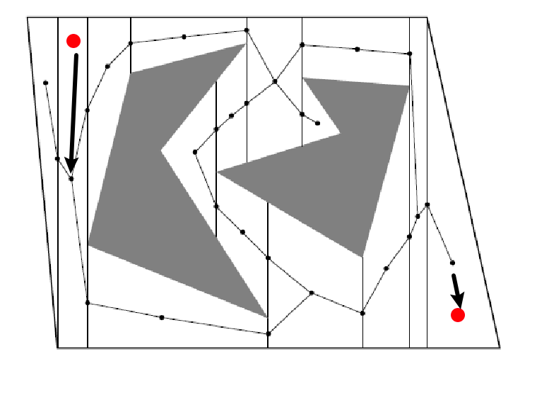
Morse Decomposition
Morse Decomposition: but it turns out you can compute step 1 even more efficiently and a in more generic way: a cell decomposition consisting of vertices that changed connectivity
- consider a line segment sweeping through
- if it encountered a vertex and the line segment splits into “two segments” merged into one, then we have a critical vertex
Visually:
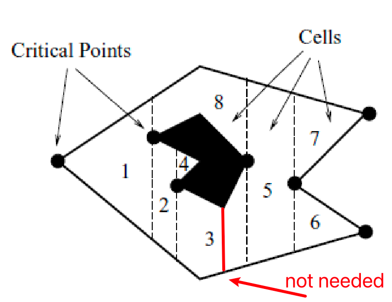
where the red line is not there because when sweeping from the critical point on its left, that segment still remains the same segment. Until we reach the region 5, where it merged with the upper segment = thats a critical vertex.
The upshot is that this produces fewer cells but is still complete.
However, cells themselves may not be convex anymore (so we might need to another decomposition + planning within those cells)
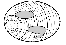
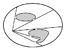
But this is more general: if you consider different slicing functions:
| Circular | Radial | Square |
|---|---|---|
 |
 |
 |
This is useful for coverage tasks in reality, since some robots might prefer to move in a certain way (e.g., circular).
Visibility Graphs
The previous method aim to give you some path, but what if we want to get an optimal/shortest path?
Consider finding optimal path using roadmaps in the following graph:
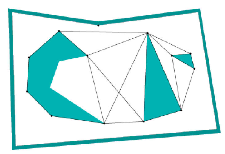
The observation is that shortest path will always include segments shown above: along the obstacle or straight lines connecting vertices.
A (reduced) visibility graph $\mathcal{G}$ is a roadmap using vertices of the C-space obstacles. Specifically:
- we consider obstacle vertices that are locally convex (interior angle less than $\pi$) as nodes
- we consider obstacle edges + collision-free bi-tangent edges between these vertices as edges
So this roadmap above basically consists of:
- obstacle vertices
- obstacle edges
- collision-free bi-tangent edges
Properties of Visibility Graph:
- $\mathcal{G}$ preserves accessibility if every point in $Q$ is within sight of a node $\mathcal{G}$
- $\mathcal{G}$ preserves connectivity if the graph is connected
- graph search on this will give you the shortest path
Visually, the optimal path search looks like:
| Given a start/end, connect to all possible vertices it can see | Then just do a graph search algorithm |
|---|---|
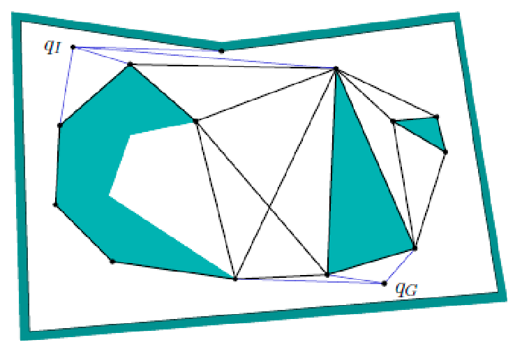 |
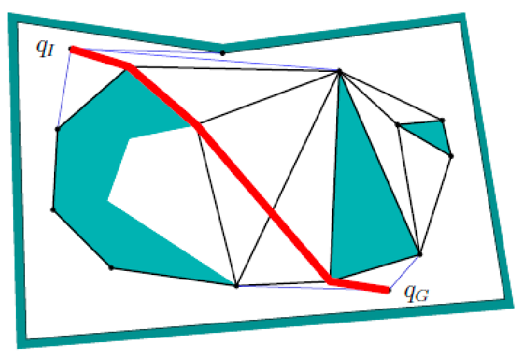 |
Efficiently Constructing Visibility Graph
How do we construct such visibility graph? The difficult part of this roadmap above is adding in the bi-tangent edges.
The idea is to do a rotational sweep from each given vertex.
- for each $v$, sort all vertices by increasing angle relative to $v$
- store a list of obstacle edges that intersected by the sweep line (sorted by which edge collide first with the sweep line)
- by how we are updating this list, we can efficiently find the bi-tangent edges
So this gives:
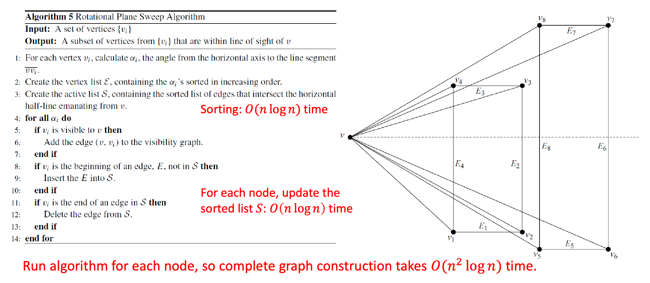
where in the above image, we will be checking vertices in the order of $v_3,v_7,v_4, …$.
On a high level, this algorithm does this:
-
initialize and check all the obstacle edges we are intersecting in $S$ (i.e., $E_4, E_2, E_8, E_6$)
-
at the next vertex (e.g., $v_3$), we will
- check what edges its connected to, i.e., $E_2, E_3$
- if these edges were already in the list, delete them = we seen them before, we are exiting now (i.e., $E_2$)
- if these edges were not in the list, add them to the list (i.e., $E_3$)
-
how do we know if the current vertex we are looking at is visible? You will need to do two checks
- make sure the segment between $v$ and $v_i$ does not intersect the first edge in list $S$
- this can actually be done in $O(1)$ time:
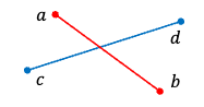
- if there is an intersection, then two vertices of one segment lies on the opposite sides of the other segment
-
this translates to if $ccw(a,b,c)$ and $ccw(a,b,d)$ have different signs:
\[ccw(p,q,r) = \begin{vmatrix} p_x - r_x & p_y - r_y \\ q_x - r_x & q_y - r_y \end{vmatrix}\]
- this can actually be done in $O(1)$ time:
- make sure the two edges at $v$ are no the same side of the sweep line
this can thus be done in $O(1)$ time.
- make sure the segment between $v$ and $v_i$ does not intersect the first edge in list $S$
Maximizing Clearance
Visibility graph gives you shortest path, but they are close to the obstacle so they may not be safest route.
A maximum-clearance roadmap tries to stay as far as possible from $\mathcal{Q}_{obs}$
Starting from a simple case: How to maximize distances from a set of points? Consider drawing perpendicular bisectors between neighboring point pairs:
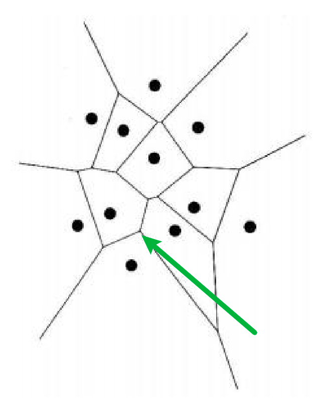
from there:
- green arrow = bisector intersections are equidistance from thre points
- other bisectors segments are equidistant from the closest two points
But how do we generalize this to obstacle regions?
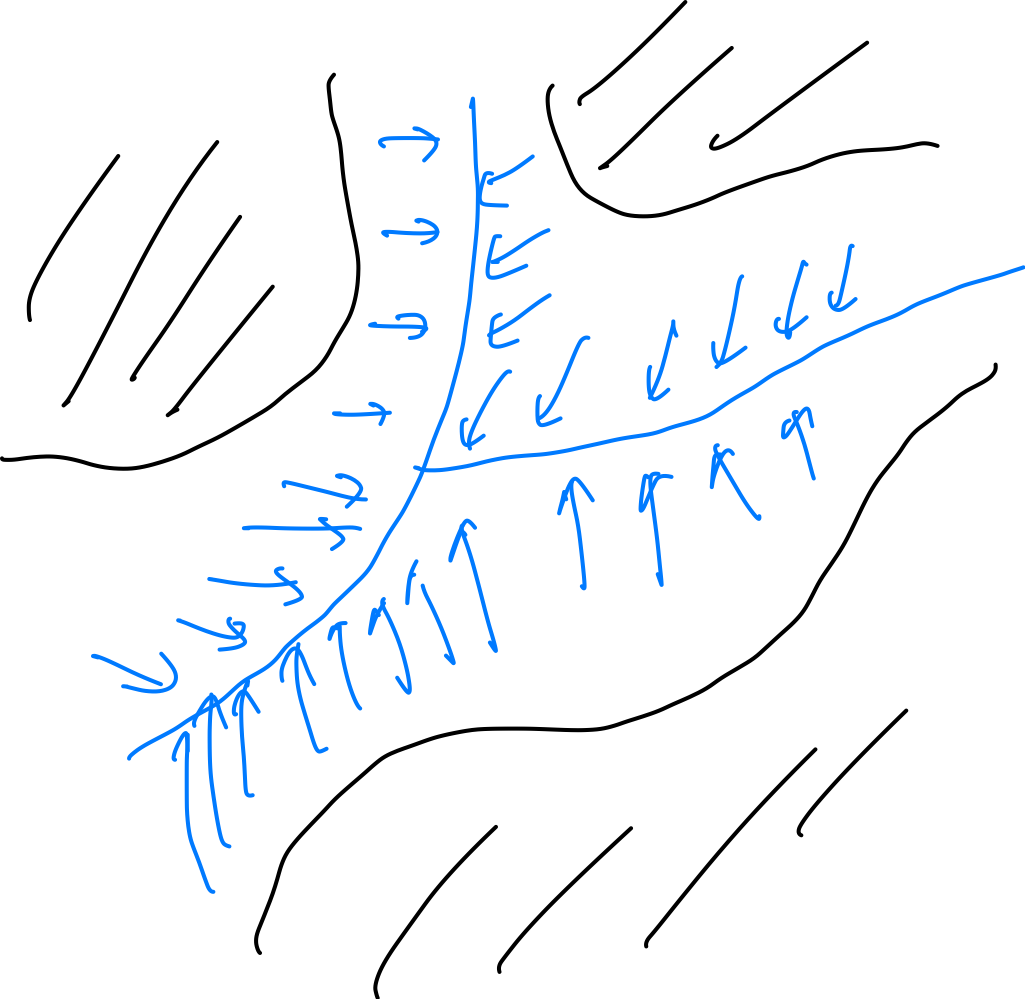
Generalized Voronoi Diagrams
To construct something like this, we need to consider accessing a distance/cost function, and consider three things:
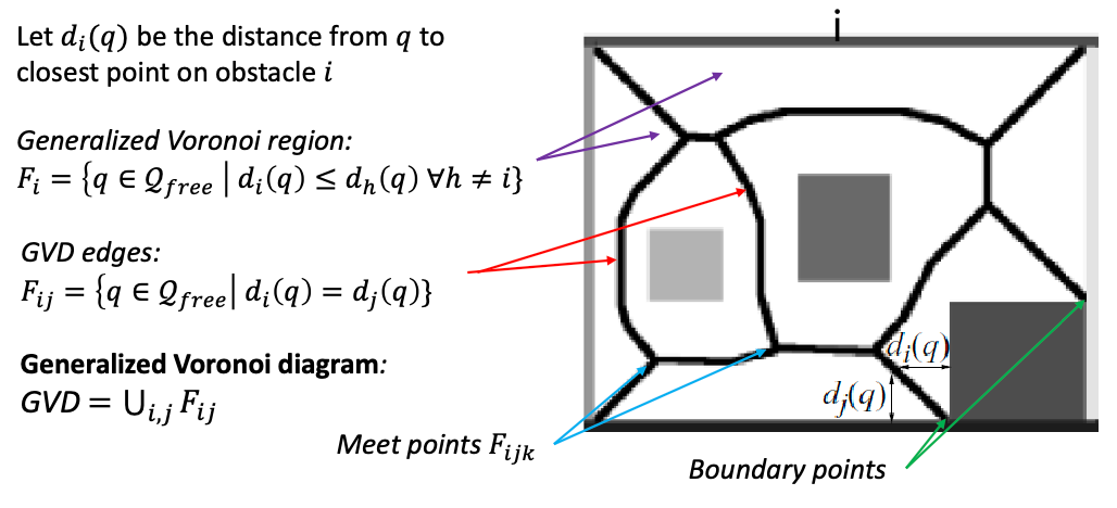
where we consider:
- Generalized Voronoi region $F_i$: the set of coordinates/points where they are closer to obstacle $i$ than any other obstacles in the diagram (the boundary of the environment is also treated as an obstacle)
- GVD edges: set of the above points where they are equidistant from two obstacles
- GVD: set of the above edges
Deformation Retracts
Here, we show that GVD are also valid roadmaps being accessible and connected. The trick is to show that $\exists$ some function that maps from any point in the free space to the GVD.
Claim 1: Given any point in the free space, we can move to the GVD by increasing distance away from the nearest obstacle
Proof:
- given a distance function $d(q)$ and an initial position $q$
-
a path $c$ to GVD from $q$ satisfies:
\[\frac{dc}{dt} = \nabla d(c(t)), \quad c(0) = q\]where we are imaging $c(t)$ being a path parameterized by $t$ that moves from $q$ to GVD.
So we can numerically find GVD by doing gradient ascent, until being equidistance from at least one other obstacle.
Deformation Retraction: a function such that give any position in free space at $t=0$, it needs to spit out a path that moves it to GVD at $t=1$:
\[h: \mathcal{Q}_{\mathrm{free}} \times [0,1] \to \mathcal{Q}_{\mathrm{free}}\]such that:
- $h(q,0) = q, \forall q \in \mathcal{Q}_{\mathrm{free}}$
- $h(q,1) \in \mathrm{GVD}$
- $h(q,t)$ is continuous in $t$
- $h(g,t) = g, \forall g\in \mathrm{GVD}$, i.e., it stays on the GVD
Using the two above properties/definitions, this means GVDs is a deformation retract of $\mathcal{Q}_{\mathrm{free}}$. Visually, all free points (blue) goes to the GVD:
Therefore, a deformation retract is a roadmap, which satisfies accessibility and connectivity. In fact, the function $h$ above directly describes how to get to the GVD from any point in the free space.
Constructing GVDs
So how do you construct GVDs? This is actually a highly studied problem in computation geometry.
A basic implementation considers the following three cases:
- being equidistance for edge-edge pairs
- being equidistance for edge-vertex pairs
- being equidistance for vertex-vertex pairs
and they you need to generate an equidistant curve (yellow) for each of the above cases and stitching them together:
basic implementation will take $O(n^{4})$ time.
Some famous algorithms for constructing GVDs are:
- Point approximations: Discretize obstacle boundaries into finite sets of points, then find all possible perpendicular bisectors and intersections
- Fortune’s algorithm: Push a sweep line through the space and trace out equidistant edges from points already seen
- Divide and conquer: Recursively divide points into sets of two, build separate GVDs and then merge them together
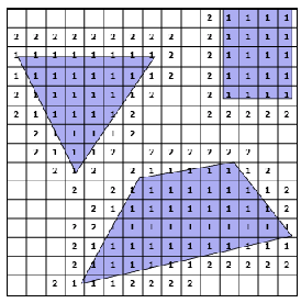
Brushfire Algorithm
But under some special cases, we can actually compute GVDs more efficiently:
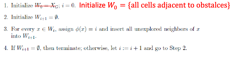
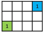
If we have a grid environment, we can actually efficiently compute GVD using the wavefront algorithm.
Brushfire Algorithm: if we are in a grid world, we can imagine the cells on the obstacle’s boundary expanding until wavefronts collided each other
- if a square was just now expanded but another wavefront want to expand it next, it is GVD cell (the 2-cells in the example below)
- if both wave fronts want to expend it, it is GVD cell (the 3-cells in the example below)
So the algorithm is simply:
Visually, we basically get the yellow cells being the GVD:
| Step 0 | Step 1 | Step 2 |
|---|---|---|
 |
 |
 |
note that visually you may feel like some cells are not really “GVD”, but this is basically because you are approximating the space via discretized cells. In practice, we just imagine we have a “thick GVD line”.
In a more complicated case:
| Step 1 | Step 2 | Step 3 | Step 4 |
|---|---|---|---|
 |
 |
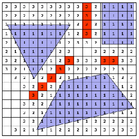 |
 |
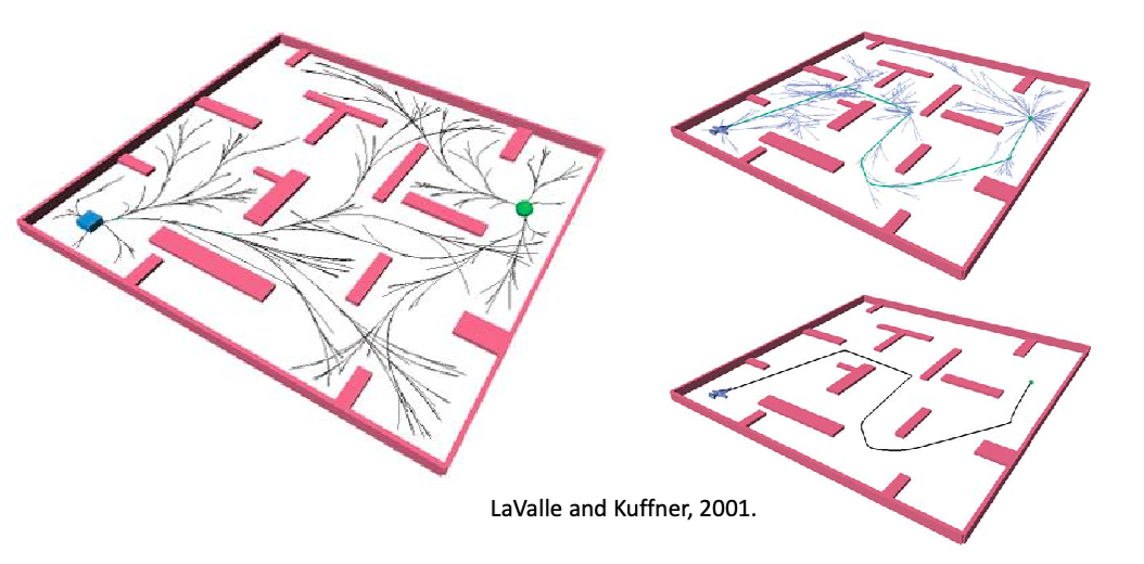
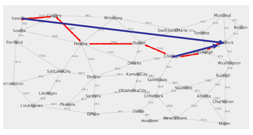
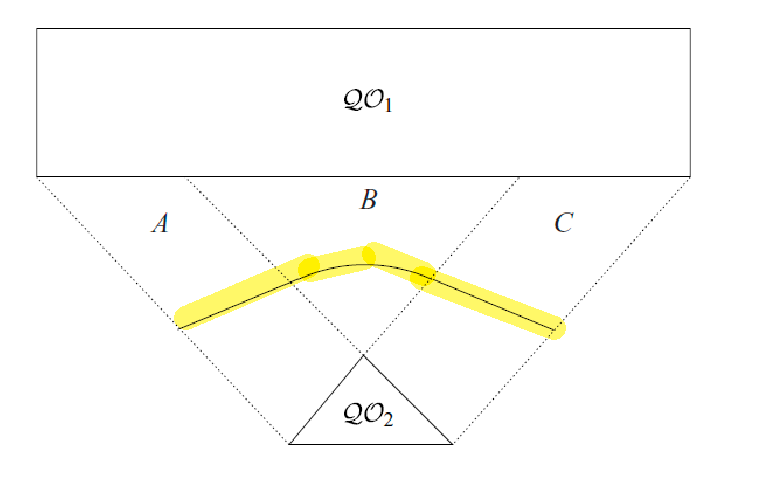
Probabilistic Roadmaps
The previous section does planning in the workspace. This is often low dimensional, mostly polynomial space:
In reality, we might need to directly plan in the configuration space of the robot (e.g. with many joints) = find a path in a high dimensional space, and the space might not even be Euclidean. In general:
-
Planning in high-dimensional and/or non-Euclidean spaces is hard
-
Constructing high-dimensional and/or non-Euclidean spaces is hard
But the idea is appealing: Maybe we construct a roadmap in the configuration space, by sampling some conllision-free configurations and connecting them
- in high dimensional space, directly figuring out the free $C_{\mathrm{free}}$ is hard = cannot easily use methods in the previous section
- since we will be using sampling methods, they have weaker optimality and completeness guarantees
- but it turns that that they are very practical for real robotic problems (many robot joints, complicated obstacles)
Sampling Based Methods
While it is hard to compute obstacles' boundaries in high-dimensional space, it is easy to check if a sampled point is in collision or not. So the idea is to:
Probabilistic roadmaps (PRM) attempt to build a roadmap in the C-space by sampling nodes coarsely and sampling edges finely in the configuration space, and add these nodes/edges to the roadmap if they are collision-free
Since sampling methods can be stochastic, we consider propoerties such as
- Resolution completeness: If a solution exists, guaranteed to find it through deterministic (e.g., grid) sampling given some sampling resolution
- Probabilistic completeness: Guaranteed to find solution if you have enough samples (i.e., high resolution)
So how do you construct such a PRM? On a high level:
- Randomly generate robot configurations (e.g., from a uniform distribution) and add as nodes to the roadmap if collision-free
- can also be generated deterministically, or with some heuristics
- Attempt to connect nodes to nearby nodes with local paths (e.g., segments), which is controlled/generated by a local planner
- the local planner is often also a sampling method, that randomly considers edges and see if it is collision free
- to do search, add initial and goal configurations to the roadmap and connect them using the local planner
- perform graph search as usual = since now we have a roadmap graph
So implementation wise
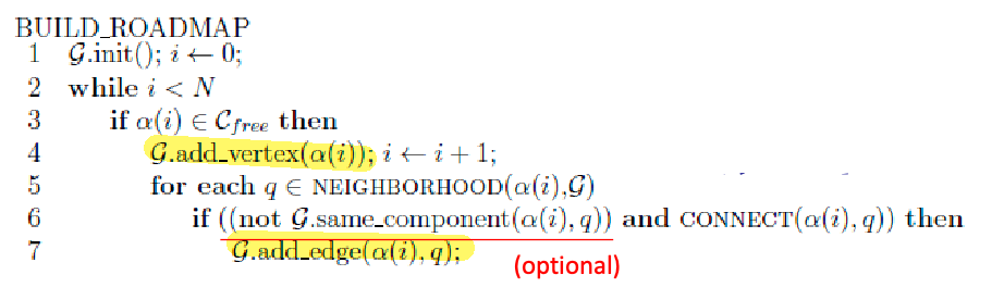
In this algorithm
- We are given or can generate a sequence of sampled vertices $\alpha$ (note that this sequence can be infinite)
- We find existing vertices in the neighborhood of $\alpha(i)$ and consider potential edges
- simple version: add if collision-free, discard if not
- more complicated version: we may also want to minimize the connectivity while keeping the same number of connected components = have a sparser graph so that planning is a bit easier
Note that similar to the previous motion planning sections, we will not return optimal paths, but will try to return feasible path whenever the task is solvable.
Visually, probabilistic roadmap looks like:
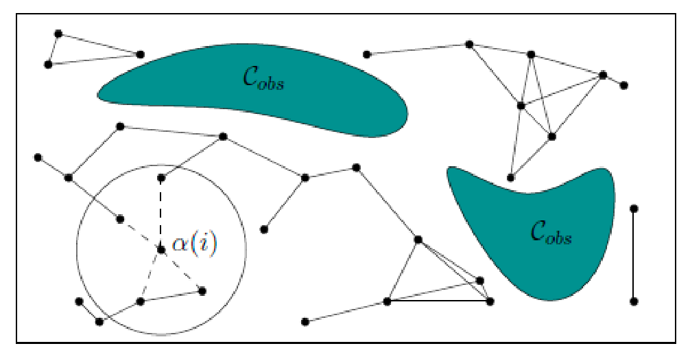
Notice that, because we could have only little samples, there can be multiple disconnected components. Therefore we may say “no path exists” if your initial and goal state are in different (disconnected) components.
There are many possible fixes, which we will discuss later. But at this point, you may question:
- How do we sample configurations?
- Do you really use uniform random sampling? If not, what kind of bias, if any, should we use?
- How do define a “neighborhood” of a vertex?
- How to efficiently perform collision checking given a configuration?
Distance Metrics
Since we needed to search in a neighborhood, we first need a distance metric:
A metric space is a set $X$ with a metric $d: X \times X \to \R$ satisfying the following:
- non-negativity: $d(a,b) \ge 0$
- reflexivity: $d(a,b) = 0 \iff a=b$
- symmetry: $d(a,b) = d(b,a)$
- triangle inequality: $d(x,z) \le d(x,y) + d(y,z)$
some useful properties of metric space include:
- a subset of a metric space $X$ is also a metric (sub)space, if you use the same metric as $X$
- if you have a vector space, you can simply use norm $\vert \vert x\vert \vert$ as the metric to obtain a metric space: $d(x,y) = \vert \vert x -y \vert \vert$
-
$L_p$ metrics is a valid metric if you consider euclidean spaces
\[d(x,x') = ||x - x'||_p = \left(\sum_{i=1}^n |x_i - x_i'|^p \right)^{1/p}\]and a max norm.
\[d(x,x') = ||x - x'||_\infty = \max_i |x_i - x_i'|\]
But what about non-euclidiean space such as $\mathbf{S}^1$? For example:
\[d \left(\theta_{1} = 0 , \theta_{2} = \frac{\pi}{2} \right) = ?\]one approach is to consider $\theta \in [0, 2\pi]$, using $L_2$ is probably still a valid metric. But the problem is that it would say $d(0, 2\pi) = 2\pi$, although intuitively it should be zero.
Therefore, one approach we often do is to:
- first embed this to a euclidean metric
- then consider using $L_p$ distance
For instance, a striaght-forward method is to consider the following embedding in $\R^{2}$ space:
Then simply:
\[d \left(\theta_{1} = 0 , \theta_{2} = \frac{\pi}{2} \right) = \left\| (1,0) - (0,1) \right\|_p\]would work. (however, this embedding method often distorts the actual distance between angles, which in this case is curved).
Finally, another useful property of metric space is that, if $(X,d_x)$ and $(Y,d_y)$ are metric spaces, then:
- consider $Z = X \times Y$
- coefficient $c_1, c_{2} > 0$
define distance:
\[d(z, z') = d((x_1,y_1), (x_2,y_2)) = c_1 d_x(x_1,x_2) + c_2 d_y(y_1,y_2)\]then $(Z, d)$ is also a metric space
This is very useful, because our robot has each joint in $SE(2)$. This means:
\[d(q, q') = c_{1} \left\| (x,y) - (x',y') \right\| + c_{2} d_\theta(\theta, \theta')\]given some valid $c_1, c_2$, is also a metric space. In practice, weights $c_1, c_2$ need to be carefully chosen to ensure the relative importance of translation/rotation is balanced.
Pseudometrics
Sometimes (in practice) it is sufficient to define functions that behave almost like metrics but violate one (or more) of the metric properties
For example, you can measure distance in robot’s configuration as the physical distance in their actual workspace:
\[d(q_1, q_2) = d(\mathrm{FK}(q_1), \mathrm{FK}({q_2}))\]this is not a metric, because it violates reflexitivity: $d(q_1, q_2)=0$ could happen even for $q_1 \neq q_2$.
But why would maintaining some of the metric properties be useful? For example:
- consider computing the neighborhood during the PRM algorithm
- using this metric, you could end up with two very different configurations $q_1,q_2$ that have zero distance. This is therefore considered “neighbors” by your metric, even though the two configurations is far from each other.
$k$-D Trees
Before finally diving into the neighborhood computation algorithm, we need to learn about some efficient data structures to find nearest neighbor fast. An naive approach would require $O(n^{2})$ time to figure out the nearest neighbor for each vertex.
Idea: construct binary tree to partition space into “halves”, and then during search we can quickly cut down the search space by halves each time
Practically, you would need to sort the points along each dimension, and then each split means: 1) traverse tio left child if the point is left/below the current node, 2) traverse to right child if the point is right/above the current node:
| Input 2D space | $k$-D tree |
|---|---|
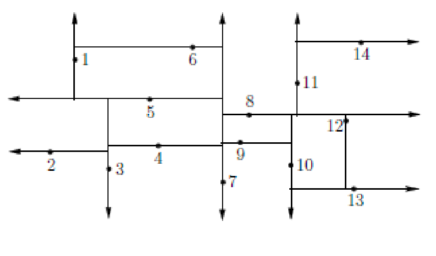 |
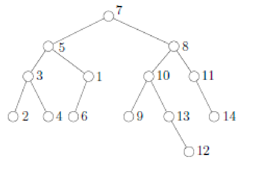 |
For example, if we have a target point $x$ that sits right next to node 14, then the search process would be:
- start at root node 7. According to the left image, node 7 partitions the space into left and right
- since $x$ is on the right side we, we go to the right child = node 8
- node 8 splits the space into above and below
- since $x$ is above, we go to the right child = node 11
- …
- finally, we reach node 14
In a nutshell: $k$-D tree sorts and stores $k$-dimensional points in a binary tree, where each node corresponds to the median point along a dimension. This will take $O(kn \log n)$ time to construct.
- if we are dealing with $k=3$ dimensions, then this tree would split by “planes” instead of a “lines” as shown above
- with the PRM algorithm, $k$ would represent the dimension of your C-space
But what if we consider the following case:
| Input 2D space | $k$-D tree |
|---|---|
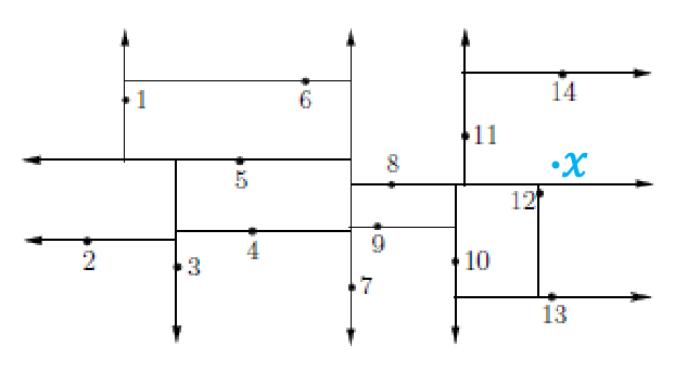 |
|
Then naively our search sequence would be $7 \to 8 \to 11 \to 14$. But we can see that the nearest neighbor is actually 12!
If our target point $x$ is closer to a boundary than the current nearest neighbot, then it means there could be nodes on the other side of the boundary that is closer (e.g., imagine there was a node right on the boundary).
- basically, at every parent (that has both children) we need to ask this question
- if the answer is yes, then during backtracking we need to consider searching the other side
Therefore, we also need to consider unwinding recursion and move back up the parent while doing checks to be completely correct:
| Step 1 | Step 2 | Step 3 | Step 4 |
|---|---|---|---|
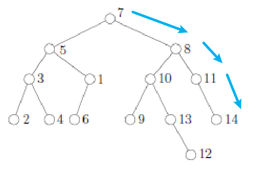 |
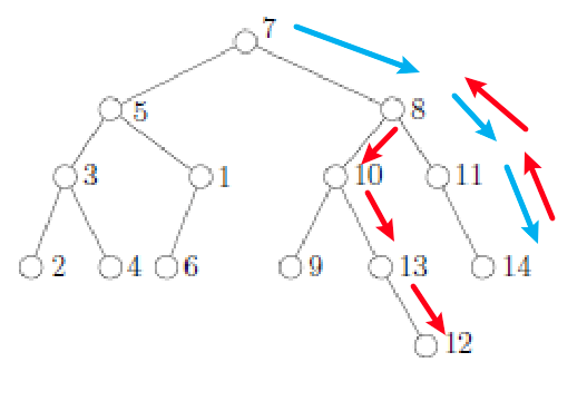 |
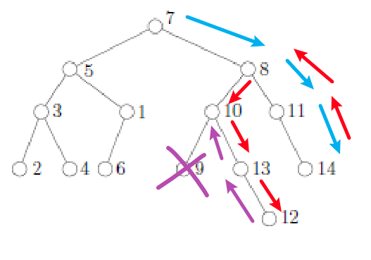 |
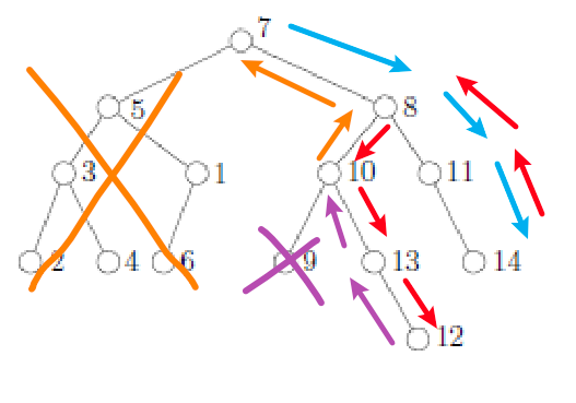 |
where:
- we start at node 7, and do a normal search to end at node 14. This is the current neighest neighbor.
- we backtrack to the first parent node that has a child = node 8. Since the distance to the boundary of node 8 is closer than the distance to the current NN (node 14), we search the other side of node 8 = node 12. This is closer!
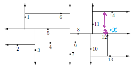
- we backtrack to node 10. This time, the distance to the boundary of node 10 is not closer than the current NN (node 12). This means we don’t need to search the other side of node 10
- we backtrack to node 7. Similar to above, we don’t need to search the other side of node 7 since its distance to the boundary is further.
- return node 12
In total, the average runtime for search is $O(\log n)$!
Vertex Neighborhood
So how can we use the $k$-D tree to obtain neighborhood of a vertex? We can:
- find nearest $k$ instead of the top-1 nearest (by additionally keeping a priority queue during the search)
- find nearest $k$ component: first find $k$-nearest nearest components, and then for each component find the nearest node
- radius: take all points within a ball of a set radius centered at $x$
- Visibility: Take all points that are visible from $x$ (analogous to the Visibility Graphs)
Here we expand on the visibility idea: can construct small roadmaps (little number of vertices) that still sufficiently cover the C-space:
| Need Neighborhood graph of $q$ | Example Output |
|---|---|
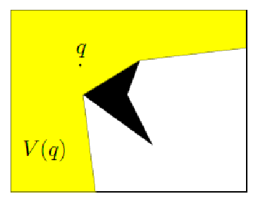 |
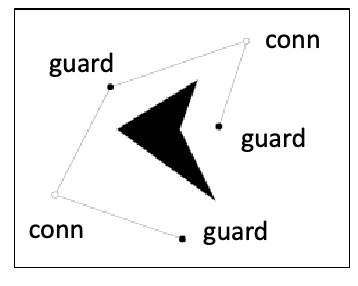 |
why is this useful: reduce connectivity again to cover large C-space with low number of nodes/edges. How does this work?
Idea: Given a vertex, its nerighbor vertex set is divided into guards and connectors:
- a guard veretx is not allowed to see any other vertex in the neighborhood
- a connector vertex must connect at least two guards
after this definition of vertices, we can have a very space graph by:
- a new vertex is considered if it’s a guard or
- a new vertex is considered if it’s a connector and it connects guards in different components
- otherwise, discard this vertex
This can clean up the neighbor set to make our edge connections/final graph a lot sparser, while still covering the C-space.
Collision Detection with Sampling Methods
Now we have methods to sample and find candidate vertices for connections. How do we check if a node/edge is collision free?
If we are considering collision detection in workspace (with arbitrary complex obstacles):
-
map the obstacles (with complicated shape) to workspace, and consider simple bounding regions
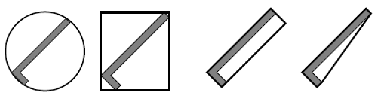
but of course, these are over-conservative.
-
then, the idea is then to consider:
- if no collision in bounding regions = no collision
- if there is, draw more fine-grained regions and repeat upto some iterations
some version of this is probably used in
pybullet
But the problem is we are planning in the high dimensional configuration space + the robot/obstacles are of complex shapes (e.g., highly non-convex)
Is there a simple approach to do collision detection? Some intuitive approach include:
Local Planner and Path Collision Detection
But in most C-space environments, we do NOT have a closed expression for the position of the obstacles. However, we can efficiently compute if a point is inside an obstacle.
So how does a local planner decide if an edge would collide with obstacles?
Again, very simple ideas include:
- draw only straight lines and check for collisions by sampling.
- this very faster but succeed less.
- to be more successful you may require denser sampling nodes.
- Slower, better planners might consider things like “curved paths”, etc.
Visually: you basically do this given that you want to (try to) connect $q$ and $q’$:
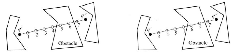
so obviously some design choice is:
- step size: too small and each check will be slow, too large and we may miss collisions
- can change step size to be adaptive, etc.
Sampling Strategies
Finally, how do we sample configurations (not too many and not too few) to construct roadmaps? Before, we kind of assumes we will be doing uniform sampling. For example, after collision detection of the nodes we could get to:
but the runtime and success rate of entire PRM procedure will have high variance.
More specialized sampling methods (e.g., using some heuristics) may be better in certain adversarial environments
Dispersion Sampling
This is actually a deterministic sampling algorithm
Idea: place more samples to shrink the size of the largest uncovered area
To do this, we first need to measure “the size of uncovered area”
The dispersion of set of samples $P$ is:
\[\delta(P) = \sup_{x \in X} \min_{p \in P} d(x,p)\]so what is this? This basically gives me the maximum distance to its nearest neighbor
- imagine computing the distance of some coordinate $x$ to its nearest neighbor
- then re-position your $x$ to maximize the above
Visually you would need to place your $x$ to be the center of the following yellow regions:
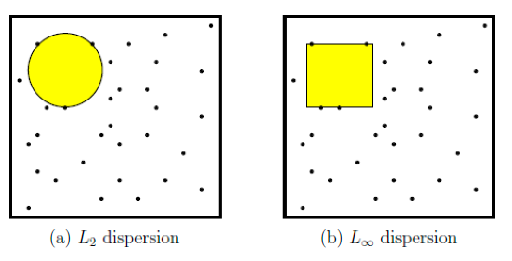
In fact, by this definition, distributing samples in a uniform grid minimizes dispersion. But that requires pre-defining how many grids to use.
So the proposed method is really aiming to achieve this while allowing you to continuously generate more samples
- because each new sample is added to minimize dispersion, this is resolution complete
- again, this can be done deterministically
Examples of algorithms that does this include
| Halton Sequence | Hammersley Sequence |
|---|---|
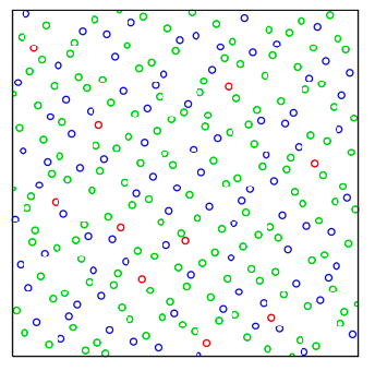 |
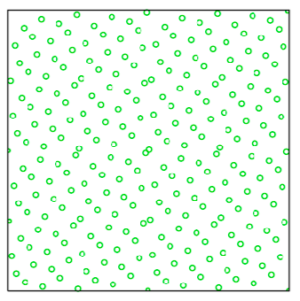 |
Connection Sampling
Previous methods are all “unbiased”: they do not really care about (e.g., the obstacles in) the environment. This can be a problem if we have narrow regions that is crowded with obstacles = likely to get disconnected components.
Idea: increase/generate more vertex samples near vertices that have weak roadmap connectivity
So we can selectively sample near such vertices to increase the density of the roadmap and try to increase roadmap connectivity:
- assign probabilities to each vertex based on heuristics like vertex degree (relative to rest of graph) or rate of failed edge connections
- when sampling, pick an existing vertex according to these probabilities and then sample in a neighborhood around it
OBPRM
A prime example that modifies the sampling procedure above and have a good practical performance is OBPRM
Idea: when you sampled $\alpha(i)$ that has a collision, instead of discarding it, sample some nodes in random directions from $\alpha(i)$. So its biased to sample near boundary of the obstacles.
Visually
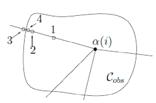
So that the roadmap at the end will look like this:
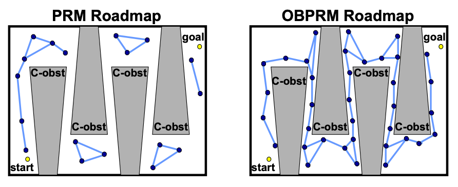
where for the PRM roadmap we were using the algorithm described in Sampling Based Methods and used uniform sampling.
Other Sampling Strategies
Some other algorithms that was useful from research:
-
GVD Sampling: We could could have a bias to get samples away from obstacles.
- We can approximate GVD by sampling uniformly, but perturb them to increase their distance away from obstacles
- to do the above we need to map back to constructing GVD in the workspace
-
Gaussian sampler: Generate $q_1$ via uniform sampling, $q_2$ from a Gaussian distribution centered at $q_2$
- Discard both if both are free or in collision; otherwise, keep the free one
-
Bridge test sampling: Generate $q_1$ and $q_2$ via uniform sampling, and if both in collision, consider their midpoint; keep if free
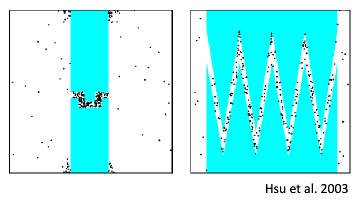
Postprocessing Queries
Given a query/solution that is already found, we can postprocess it to find some shortcuts so that the resultant path is further optimized
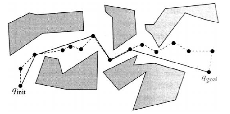
On a high level, you can
- Find a node $q_0$ closest to start that can connect directly to the goal
- Then find a node $q_1$ closest to start that can connect directly to $q_0$
- … repeat until start is directly connected to the shorter path
Single-Query Planners
For PRMs, our goal was to construct a representation of the free C-space that can be used for planning. Specifically, they are usable: once constructed, you can use them for multiple queries of different start/goal pairs.
Here, we diiscuss single-query planners that are designed to solve a single query (start/goal pair) as efficiently as possibl, i.e., in the C-space, find me a path from $q_{\mathrm{start}}$ to $q_{\mathrm{goal}}$.
As you will see, these algorithms will be:
- again sampling based, but will have bias (towards reaching the goal state) and exploration (to avoid local minima) stages
- is in practice more efficient to run than PRMs
Grid-Based Roadmap
The first (not-very single-query-related) idea is to use a grid-based roadmap. The implementation, however, can be done in a single-query manner.
Simple Grid-based Roadmap: given a start $q_I$ and end $q_G$ configuration, overlay a grid (ignoring the obstacles for now). Then, you can either remove obstacles after that, or you can check on-the-fly of planning if the vertices are in collision.
for collision-check, alike PRMs we will a run local planner (e.g., sample along the line and check for collision) at the neighbor vertices that you would traverse next.
| Lay a grid | Remove Collisions |
|---|---|
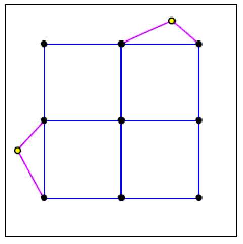 |
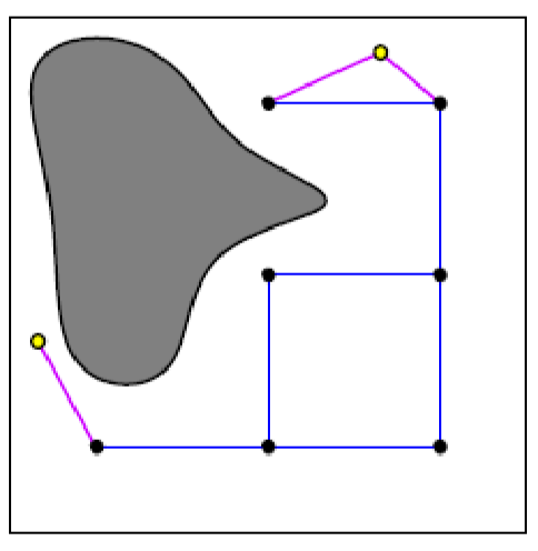 |
Problem with this approach:
- curse of dimensionality: this doesn’t scale well when you increase dimension. To keep dispersion, increasing one dimension = square the number of samples (we will cover much more efficient single-query approaches soon)
- is resolution-complete: depends on resolutions to be able to find the solutions
Practial stitches to the resoluion problem?
- just increase resolution and do again: expensive
- itereatively increase resolution between search processes
- Add new samples to the grid one (or a few) at a time
- check if the initial and goal state are in the same component (if so, done). This can be done efficiently using union-find.
Potential Functions
Besides thinking about how to construct vertices and edges efficiently in high-dimension, another concern is the cost of the search after you laid out the plan.
Searching for the path itself can be very expensive in high-dimensional spaces. Potential functions generalize heuristics (see A* Search), can be used to guide the search
for example, yuo can imaging having:
- e.g., an attractive force = distance towards the goal
- e.g., a repulsive force = distance away obstacles
but note that in C-space we often don’t know the layout, this heuristics is often just your guess. But how will this relate to the roadmap?
A peak at single-query algorithms we will see: they will consider efficient sampling based approach to explore/map out the C-space, but also guided by some cost/distance function to eventually find the path connecting the start and goal state.
From the above, you might wonder: why do we need to have exploration if I have a potential function? Suppose your guessed a potential/cost functino being the straight line distance between start and goal state:
| Unforseen Boundary | Narrow Passages |
|---|---|
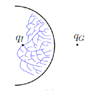 |
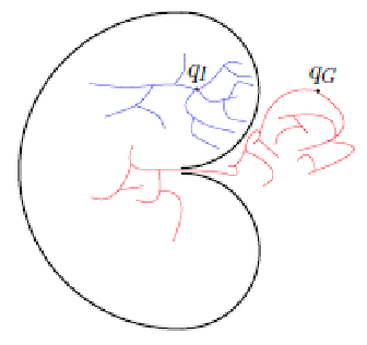 |
where:
- for the first case, really “random” exploration may be required for the search algorithm
- for the second case, you might need to also search from the goal state to be lucky
In general: finding a good potential function would require a lot of trial and errors.
Randomized Potential Fields
If we really want to use potential fields methods, there are some ways to get out of local minima. Normally, your algorithm would simply try to explore by steping in the direction to decrease potential (and eventually get stuck at a local minima).
One simple idea to add some exploration and get out of the local minima: execute a random walk
implementation-wise: perturb each coordinate by some random direction, check if potential is decreased (if not, repeat this random process for a couple of iterations)
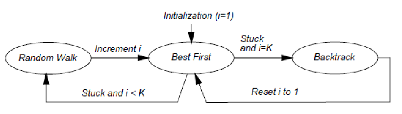
note that a backtracking step may also be used to limit the number of unsuccessful random walks.
Tree-Based Planners
Finally, we discuss the most practical single-query planners: tree-based planners.
Idea: we grow a tree by sampling (sampling vertices and connecting them), such that:
- we bias the sampling process of roadmap construction = prioritize exploring only the C-space regions that relevant to the query
- eventually it will reach the goal state = done!
On a high level, these algorithms
- are very similar steps to Dijkstra’s Algorithm and A* Search, with the main difference is they know the full graph in advance, but here we sample new vertices on-the-fly
- each step here consists of sampling a new vertex (expansion), running a local planner and inserting an edge if valid, and checking for a solution (goal test)
Expansive-Space Trees
EST algorithm: initial trees $T_{init}$ and $T_{goal}$ at the start/goal and alternatively grow trees from both sides.
- initialize two trees
- pick an existing node $q$ according to some distribution $\pi_T$
- sample a new node $q_{rand}$ near $q$ (expansion)
- if local planner say we can connect them, add $q_{rand}$ to the tree
- since we have two trees, we need to interleave some merge attemtps
- repeat from step 2 alternatively from both trees
Notice that this is much more biased than general PRM: we only sample near the current vertex and biased towards the goal/start state (by the distribution and by the merging process)
Visually, after selecting $q$ we basically do:
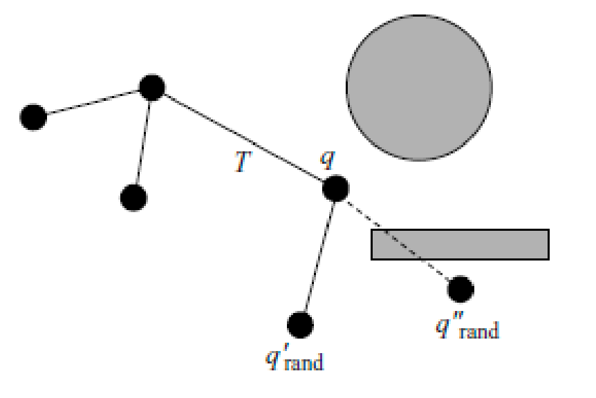
in more details:
-
how do we merge? simply treat one node in a tree (e.g., $T_{init}$) as the sampled $q_{rand}$ for the other tree (e.g., $T_{goal}$)
- so we interleave some merge attemptes with the tree growth
- eventually merge will success when the trees are close enough
- once succeeded, we are done
-
what should $\pi_T$ be = used to choose which node to expand next?
- if we want to have some exploration, this should be higher in sparser regions = reflect neighborhood density
- so this can be done in many ways, such as:
- inversely proportional to the number of nodes near $q$
- can also use other heuristics such as distance, out degree, etc.
Drawback of EST:
- we need continuously update $\pi_T$ as we expand new nodes = can be expensive.
- It is also very sensitive to how you defined $\pi_T$ and other parameters such as how often do you merge
Rapidly-Exploring Random Trees
Much more practical to uset than EST is the RRT algorithm.
Rapidly exploring random tree (RRT): instead of growing the tree blindly, we can sample $q_{rand}$ anywhere in the C-space, and “connect” them to an existing tree node $q_{near}$ that’s closest to $q_{rand}$.
- don’t need this sampling distribution $\pi_T$ to choose which node to expand
- eventually, the “connect” part will lead the trees to merge
This algoritm also
- guarantees a dense covering
- Samples may be randomly or deterministically generated
- can work by either grow one tree from $q_I$, or two trees from both $q_I$ and $q_G$ (bi-directional trees)
A bit more details of how the algorithm work
- sample a random node $q_{rand}$ (randomly or deterministically)
- figure out the closest tree node $q_{near}$
- add a new node $q_{new}$ (i.e., expansion) by taking a step size distance away from $q_{near}$ in the direction of $q_{rand}$
- if there is a collision, do not add and repeat from step 1
- if no collision from $q_{near}$ to $q_{new}$, add
- discard $q_{rand}$, and repeat from step 1
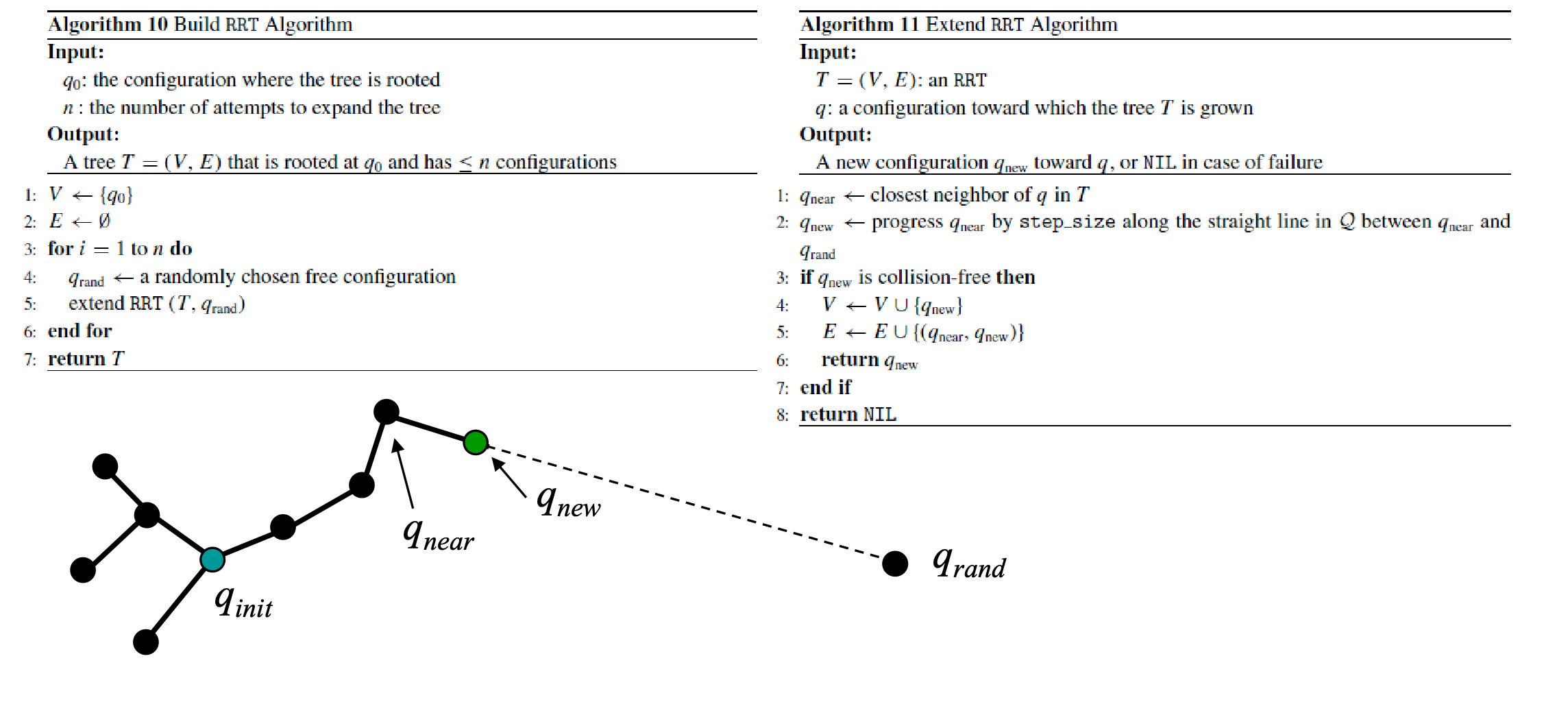
Greedy Extend RRT
While you can simply pick a small constant step size, another small change is to do this automatically and greedily.
Idea: start with one small step. If it worked, increase one step and check again. Return when we have a collision.
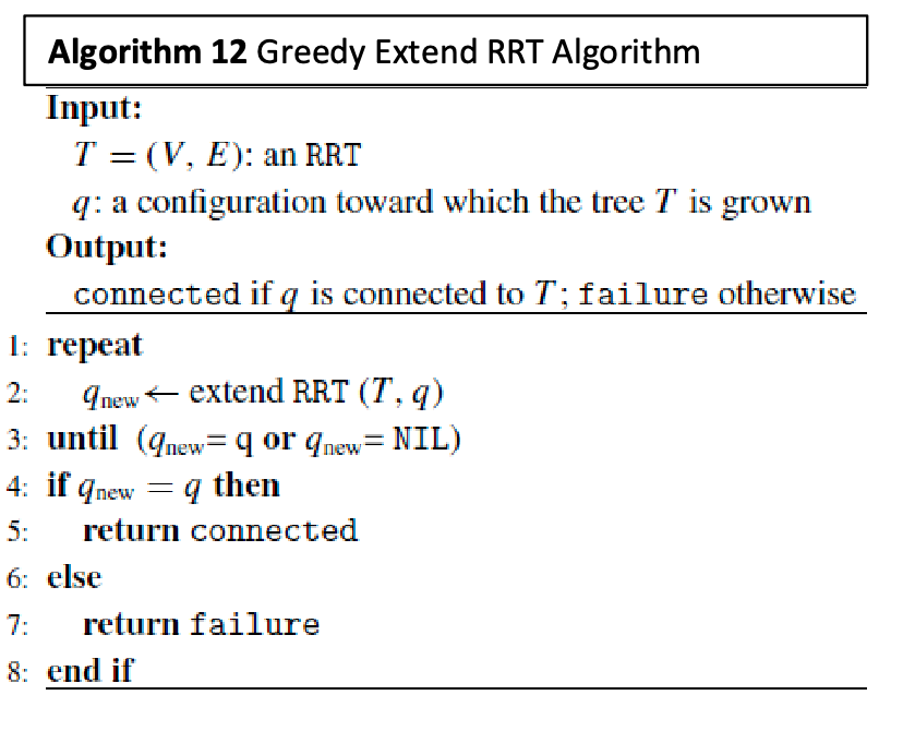
This can be used to reduce number of vertices = discard all intermediate nodes generated during this greedy extend.
Other Extend Variations
However having fewer nodes might not be always the best in this case = may make it more difficult to connect new nodes to the (sparse) tree
Idea: If we have long edges, $q_{rand}$ may be closer to an edge than a node. Then we can still connect the node, but also add a new node to the edge.
- this requires more computation = need to compute distance from a point to an edge in a high-dimensional space
- we add one new node to the existing edge and split the edge into two
So visually, you would have computed and created a new red vertex:
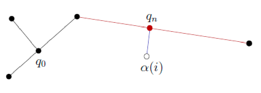
Adding Sampling Bias
Another modification that we can do to improve the algorithm is to add some sampling bias. Rather than sampling uniformly, to stick to our single-query idea, we can bias the sampling of $q_{ran}$
Idea: with a small probability $\epsilon$, set $q_{rand}:=q_{goal}$ as if its our new sample. Otherwise, $q_{rand}$ is uniformly sampled.
note that
- if we started with a single tree, this also ensures that we will connect $q_{goal}$ to our current ree
- why can’t we just do $q_{rand}:=q_{goal}$ all the time? then there is no exploration = get stuck in local minima
- so basically $\epsilon$ controls exploration
Merging RRT Trees
Finally, if we chose to grow two trees, how do we merge? Merging RRTs proceeds similarly to merging ESTs.
After growing trees for a set time, we run the merge algorithm with an upper bound on number of tries:
- suppose we expanded $T_1$ randomly and added a node $q_{new}$.
- attempt to expand $T_2$ by adding treating $q_{new}$ as its $q_{rand}$
- if fails, repat from step 1 but swap the roles of $T_1$ and $T_2$
- if step 3 failed too many times, go back to growing trees
So you basically will run this once in a while when growing your tree.
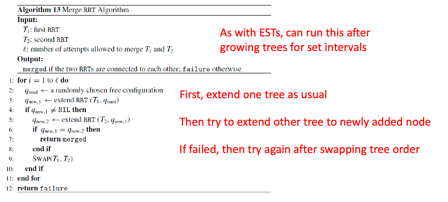
Visually you will get this green path when the two tress are close enough
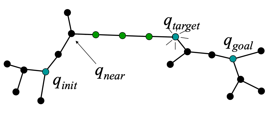
RRT Visualizations
Now we have a complete description of the algorithm, some visualizations:
| RRT Example in 2D (bi-directional trees) | RRT Example in C-space |
|---|---|
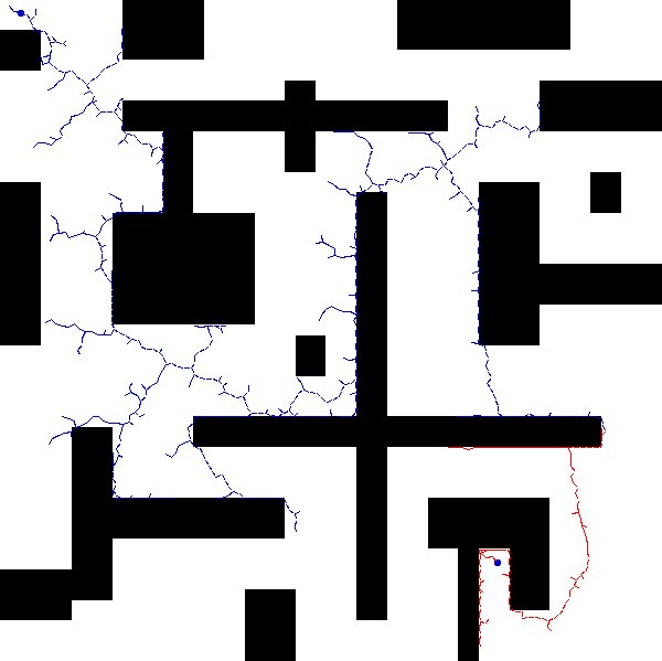 |
 |
(credit: RRT Page: Photo and Animation Gallery (lavalle.pl))
RRT Limiting Behavior
In the limit of running for infinite number of iterations, it can be proven that we can cover all places in the C-space. Visually:
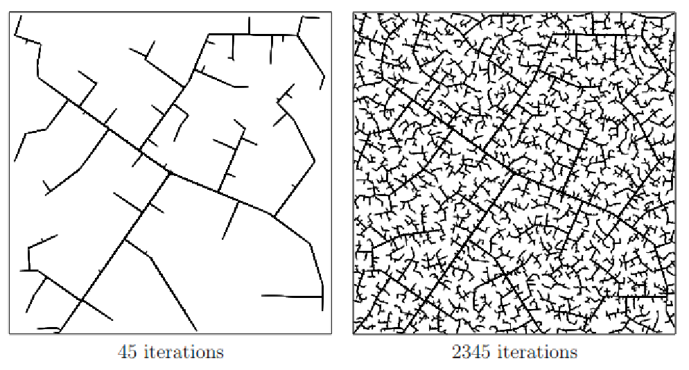
Specifically, the original paper proved that, if a path from $q_{init}$ to $q_{goal}$ exists in the free C-space:
- the expected number of iteration needs to find a path can be upperbounded
- the probability that RRT fails to find the path decreases exponentially with the number of iterations
- therefore, RRT is probabilisitically complete: in the limit that there are infinitely many nodes, the probability that a tree rooted at $q_I$ contains $q_{G}$ approaches to 1.
Growing More than Two Trees
We can also have (more) new trees grown in arbitrary or difficult parts of the C-space! This may be appealing for some reasons:
- each tree can be computed in parallel = faster computation
- instead of connecting to some start/goal state, we can just connect the trees = a more general roadmap
Some key steps you will need to do:
- uniformly sample the C-space and grow trees with EST, RRT, or any variation of the two strategies
- merge neartest tree neighrbos = can define distance as distance between representative nodes (e.g., centrooid)
Sampling-Based Roadmap of Trees
One example algorithm that does this is the Sampling-Based Roadmap of Trees (SRT). This can also be seen as an integration of both RRT and PRM, since you end up having many clusters of trees:
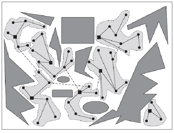
implementation-wise:
- to connect to neighbor trees together
- try one pair of nodes fro meach tree, and use a local planner to connect them
- if tailed, use RRT/EST merge algorithms (which can also grow the tree a bit)
- given some initial/end state, we can
- directly connect them to the roadmap, if they are close enough to some tree
- if not, can also grow trees from them
Note: this is more like a PRM - a multiple-query graph. In practice, if your goal is to get a PRM, then you should use traditional PRM algorithms, and use this unless you failed.
Optimality for RRT
The RRT algorithms does not have optimality, as we only aimed to find some feasible path. However, it turns out that we can modify them to achieve asymptotic optimality.
But of course, optimality = assumes there is a distance/cost metric already given.
Rapidly-Exploring Random Graph
One modification is to:
- connetc all nearest neighbors in the tree to $q_{new}$
- since this produces cycles = no longer trees but graphs
- but is proved asymptotically optimal = RRG will contain optimal path for sufficiently large node neighborhoods
RRT*
As seen in many examples, RRTs can grow many good nodes, but the edges are “not optimal”.
RRT* Idea: we grow $q_{rand}$ nodes the same way as RRT, but carefuly consider which node $q_{rand}$ should connect to.
More specifically:
- for a $q_{new}$ we just added, first connect it with all neighbors (no longer a tree as we can have cycles)
- prune the edges so that
- ensure every node in the neighborhood of $q_{new}$ has its previous parent having the cheapet cost to start
- only keep the edge to the cheaper parent
- stop until you get a tree structure
As a result, existing nodes may change parents as tree grows outward. To compare
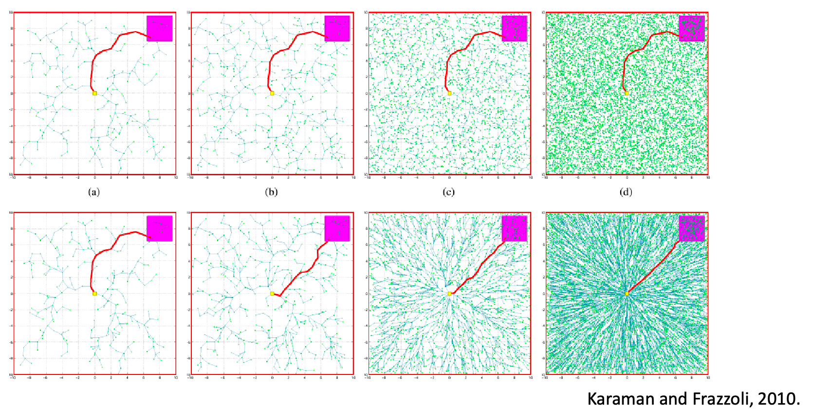
where:
- first row RRT considers random nodes and connects them = edges are in random directions
- second row RRT*: nodes are also random, but edges are pruned to be optimal w.r.t. the cost function (same function used for optimality)
Differential Constraints
So far we have really only considered path or kinematic planning: just give me a path.
The full motion planning problem also considers how the paths are followed = practical robot systems have physical constraints
Often theses are written down as differential constraints:
- constraints on velocities, directions of motion, etc.
- so written as differential equations, e.g., $\dot{x}=f(x,u)$ where $x$ is the state (e.g., current position), and $u$ is an action (e.g., control the velocity forward)
So “solving the motion planning problem” becomes: return an action trajectory $\tilde{u}$ such that the correspdoning state $\tilde{x}$ trajectory satisifes the constraints.
Can we not directly plan in the action space and do some fixes to satisfy the constraint? Not with the algorithsm discussed so far, as they consider each state being independent of each other!
- the short answer is: we can plan in the $x$-state space, but each vertex is a $u$ that satisfies the constraints. Then, given a path from start to end, we can extract the sequence of $u$ from the $x$-path.
- but before we discuss how this works, first let’s understand what kind of constraints we will have
For example: consider a simple car that has two actions: forward velocity $u_s$ and steering angle $u_\phi$. Since cars cannot do sharp turns, we constraint the velocity to be:
\[\dot{x} = u_s \cos\theta\\ \dot{y} = u_s \sin \theta\\ \dot{\theta} = \frac{u_s}{L} \tan u_\phi\]state space is $(x,y,\theta)$, and action space is $u_s, u_\phi$.
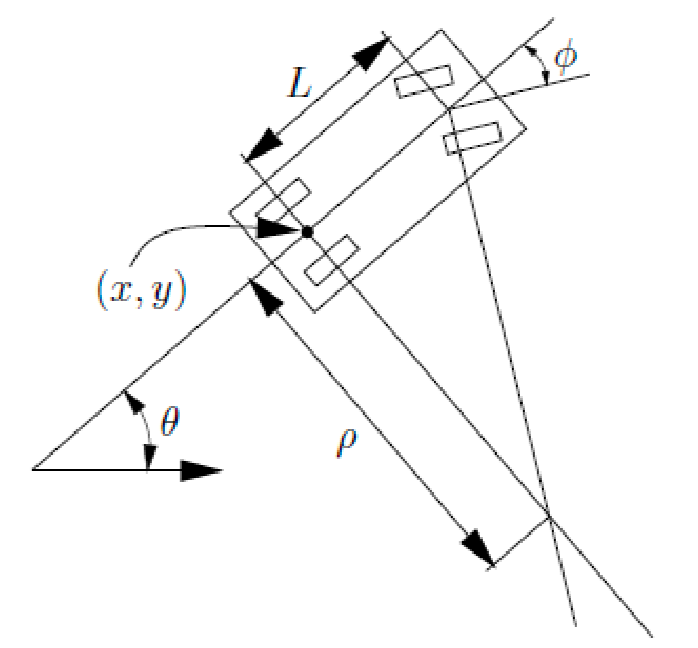
Another common example: differential drive is
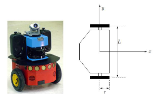
which has constraint of:
\[\dot{x} = \frac{r}{2}(u_l + u_r) \cos\theta \\ \dot{y} = \frac{r}{2}(u_l + u_r) \sin\theta \\ \dot{\theta} = \frac{r}{L}(u_r - u_l)\]So how do you do planning with this constraints?
- this becomes a nightmare for combinatorial approaches
- but turns out that sampling based approaches is more or less okay (as briefly hinted above)
Kinodynamic Planning
Idea: we plan in the $x$-state space, but each pair of vertex is connected by an action $u$ that satisfies the constraints. Then, we can extract the sequence of $u$ from the $x$-path.
So basically we consider
-
Kinodynamic RRT first samples $x_{rand}$ and finds $x_{new}$ as before
-
instead of directly do a strght line connect, the local planner will need to draw a path that solves the differential constraint between the two samples
Before Here 
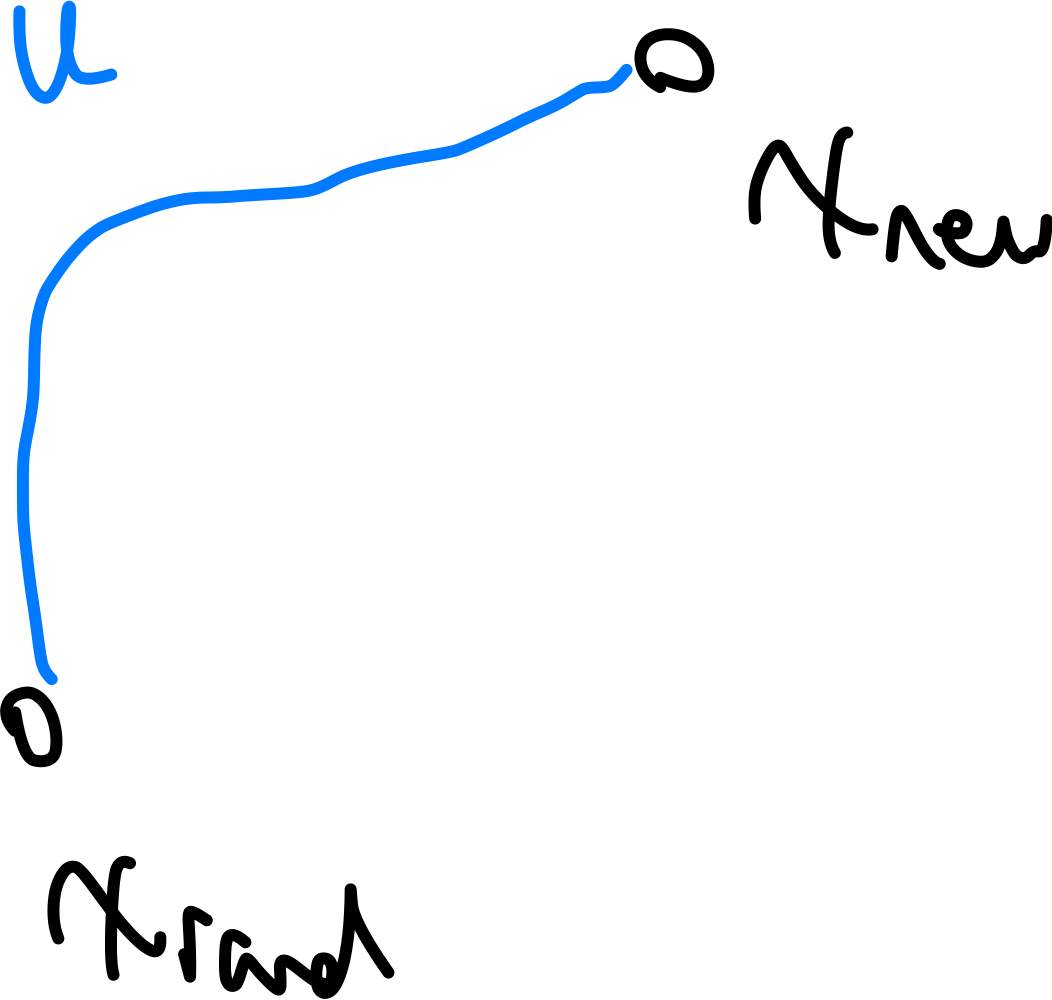
where $u$ is in the action space.
-
one we found a $x$-path, we can then extract $\tilde{u}$ as a sequence of $u$-edges.
Visually, if we only want to plot the full $x$-path, you will need to integrate over $u$ for each edge to obtain figures like below: