COMS4733 Computational Aspects of Robotics part2

[toc]

Probabilistic Models and Localization

The problem is that in reality, we can have inaccuraries of

• dynamic and unstructured environments
• noisy sensors and actuators
• inaccurate models

etc. So the goal of this section is to bring probability (e.g., confidence) into robotic modeling and algorithms

Probability and Statistics Refreshers

We denote a random variable as $X: \Omega \to \R$ map sample space outcome (e.g., dice number) to real values (e.g., 4). We then have

• in a discrete case, we have PMF $f_X(a) = \Pr(X=a)$ is the actually probability
• in a continous case, we have PDF, $\Pr(a \le X \le b) = \int_b^a f_X(x)dx$​ is probability

For multiple random variables, we have a random vector $\mathbf{X} = [X_1, …, X_n]$. This then have:

• a joint PMF being simply:

  \[f_X(x_1, ..., x_n) = \Pr(X_1 = x_1, ..., X_n = x_n)\]

  which again describes an actual probability,

• a joint PDF being:

  \[\Pr(a_1 \le x_1 \le b_1, ..., a_n \le x_n \le b_n) = \int_{a_1}^{b_1}\dots\int_{a_n}^{b_n}f_X(x_1, ..., x_n) dx_n...dx_1\]

• a marginal distribution then considers either:

  \[f_X(x) = \sum_y f_{X,Y}(x,y)\]

  for a continuous case

  \[f_X(x) = \int f_{X,Y}(x,y)dy\]

---

Important examples: Multivariate Gaussian. A n-vector $X$

\[X \sim N( \mathbf{\mu}, \Sigma), \quad \text{where } X,\mu \in \R^n, \Sigma \in \R^{n \times n}\]

this is defined by

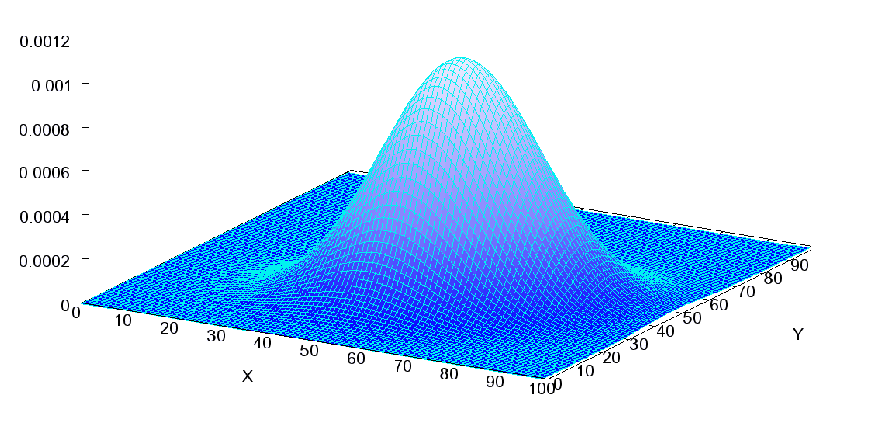
\[f_X(x) = \frac{1}{\sqrt{(2\pi)^n |\Sigma|}} \exp\left( -\frac{1}{2}(\mathbf{x} - \mathbf{\mu})^T \Sigma^{-1} (\mathbf{x} - \mathbf{\mu}) \right)\]

visually for a 2D multivariate Gaussian:

some key properties:

• linear combinations of elements of $X$​ is also a Gaussian.
• $\sqrt{(\mathbf{x} - \mu)^T \Sigma^{-1} (\mathbf{x} - \mu)}$ is the Mahalanobis distance between $\mathbf{x}$ and mean $\mathbf{\mu}$

Conditional Distributions and Independence

For conditional distribution

Discrete	Continous
$$\Pr(x	y) = \frac{\Pr(x,y)}{\Pr(y)}$$	$$f_{X	Y}(x	y) = \frac{f_{X,Y}(x,y)}{f_{Y}(y)}$$

For two RV to be independent, then:

\[f_{X,Y}(x,y) = f_X(x)f_Y(y),\quad \forall x,y\]

which is equivalent of saying $f_{X\vert Y}(x\vert y) = f_X(x)$: knowing $y$ tells us nothing extra about what $x$ could be.

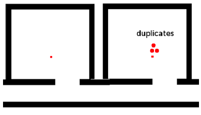
As an example, consider a bivariate uniform distribution: one everywhere inside a box:

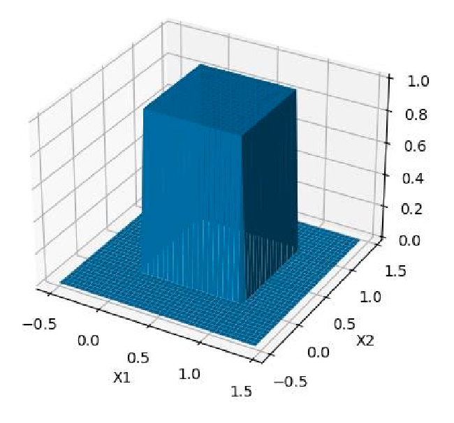
where you can check that $f_{X_1, X_2}(x_1, x_2) = f_{X_1}(x_1)f_{X_2}(x_2)$ everywhere, and that knowing $y=0.3$ or $y=0.5$ tells you nothing about $f_X(x)$.

---

In reality, independence is hard to observe. A looser version of independence is conditional independence

Conditional Independence: given a RV’s value $Z=z$, then:

\[f_{X,Y|z}(x,y|z) = f_{X|z}(x|z)f_{Y|z}(y|z)\]

we say $X,Y$ is conditional independent given $Z=z$.

Note that absolute independence may not infer conditional independence:

• $f_{X,Y\vert z}(x,y) = f_{X\vert z}(x)f_{Y\vert z}(y) \centernot\implies f_{X,Y}(x,y) = f_X(x)f_Y(y)$​ because $z$ may contain important information
• $f_{X,Y}(x,y) = f_X(x)f_Y(y)\centernot\implies f_{X,Y\vert z}(x,y) = f_{X\vert z}(x)f_{Y\vert z}(y)$ because knowing something about $z$ might break independence

Expectation and Variance

Obviously:

Discrete	Continous
$\mathbb{E}[X] = \sum_i x_i f_X[x_i]$	$\mathbb{E}[X] = \int x f_X(x)dx$

A function $g(X)$ of a random variable is also a random variable. So then you could also consider the expectation of $g(X)$ as:

\[\mathbb{E}[g(X)] = \int g(x)f_X(x)dx\]

an exercise: the linearity property of expectation

\[\begin{align*} \mathbb{E}[aX + bY] &= \iint (ax+by)f_{X,Y}(x,y) dxdy \\ &= \iint ax f_{x,y}(x,y)dxdy + \iint by f_{x,y}(x,y)dxdy\\ &= a\int xf_X(x)dx + b\int y f_Y(y) dy \\ &= a \mathbb{E}[X] + b \mathbb{E}[Y] \end{align*}\]

Then the variance is like a “second moment” but:

\[\text{Var}[X] = \mathbb{E}[ (X - \mu)^2]\]

is like measuring the dispersion of an RV’s value from the mean. We can then also show using linearity of expectation:

\[\begin{align*} \mathbb{E}[(X-\mu)^2] &= \mathbb{E}[X^2 - 2 \mu X + \mu^2]\\ &= \mathbb{E}[X^2] - 2\mu \mathbb{E}[X] + \mu^2 \\ &= \mathbb{E}[X^2] - \mu^2 \end{align*}\]

some important properties of variance. (prove them as an exercise)

• $\text{Var}[X+Y] = \text{Var[X]} + \text{Var}[Y] + 2\text{Cov}[X,Y]$, i.e., there is a “cross-term”:

  \[\text{Cov}[X_i,X_j] \equiv \mathbb{E}[ (X_i - \bar{X}_i) (X_j - \bar{X}_j) ] = \mathbb{E}[ X_iX_j] - \bar{X}_i\bar{X}_j\]

  is like how the two RV interacts with each other. So if two variables are independent of each other, then:

  \[\text{Cov}[X_i, X_j] = \mathbb{E}[X_iX_j] - \bar{X_i}\bar{X_j} = \bar{X_i}\bar{X_j}-\bar{X_i}\bar{X_j}=0\]

• $\text{Var}[aX] = a^2\text{Var[X]}$ has the scalar squared.

Finally, what if $X$ is a vector? Then

Covariance for a $n$-vector $\mathbf{X}$ is then:

\[P_X \equiv \mathbb{E}[(\mathbf{X}- \bar{\mathbf{X}})(\mathbf{X}- \bar{\mathbf{X}})^T] = \mathbb{E}[\mathbf{X}\mathbf{X}^T] - \bar{\mathbf{X}}\bar{\mathbf{X}}^T\]

visually,

\[P_x = \begin{bmatrix} \text{Var}[X_1] & \text{Cov}[X_1, X_2] & \dots & \text{Cov}[X_1, X_n]\\ \vdots & \text{Var}[X_2] & \dots & \vdots\\ \vdots & \dots & \ddots & \vdots\\ \text{Cov}[X_n, X_1] & \text{Cov}[X_n, X_2] & \dots & \text{Var}[X_n]\\ \end{bmatrix}\]

which is also symmetric, positive semi-definite matrix (i.e., $x^TP_xx \ge 0, \forall x$.)

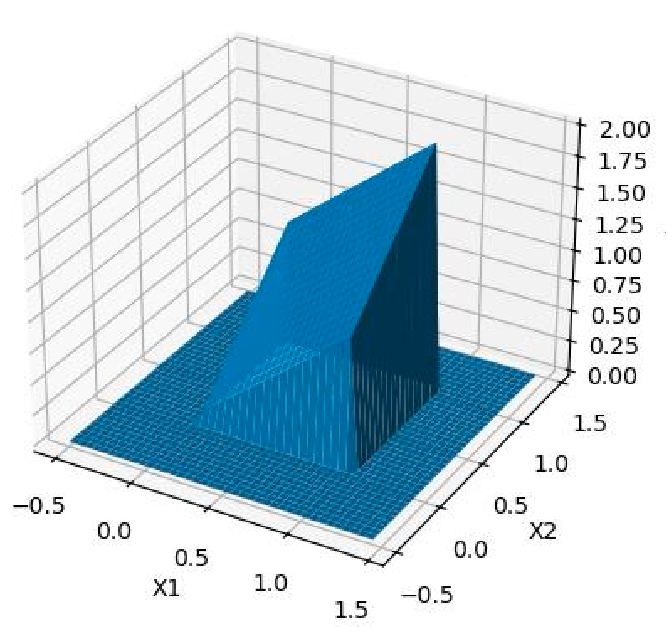
As an example, consider. a bivariate distribution

\[f_{X_1, X_2}(x_1, x_2) = \begin{cases} x_1 + x_2, & 0 \le x_1 \le 1, 0 \le x_2 \le 1\\ 0, & \text{otherwise} \end{cases}\]

visually

We can then compute:

• marginal of $f_{X_1}$:

  \[f_{X_1}(x_1) = \begin{cases} \int_{0}^1 x_1 + x_2 dx_2 = x_1 + \frac{1}{2}, & 0 \le x_1 \le 1\\ 0, & \text{otherwise} \end{cases}\]

• conditional given $x_1=1$:

  \[f_{X_2 | X_1}(x_2 | X_1=1) = \begin{cases} \frac{f_{X_1,X_2}(1,x_2)}{f_{X_1}(1)} = \frac{1+x_2}{3/2} = \frac{2}{3}(1+x_2), & 0 \le x \le 1\\ \text{undefined}, & \text{otherwise} \end{cases}\]

• expectations, which is symmetrical in this case

  \[\mathbb{E}[X_1] = \mathbb{E}[X_2] = \int_{0}^1\int_0^1 x_1 (x_1+x_2)dx_1dx_2 = \frac{7}{12}\]

• variance, again symmetrical:

  \[\text{Var}[X_1] = \text{Var}[X_2] = \int_{0}^1\int_0^1 x_1^2 (x_1+x_2)dx_1dx_2 - \bar{X}_1^2 = \frac{11}{144}\]

• covariance matrix: we know that the diagonal are the variances of individual element, we only need to find the covariances:

  \[\text{Cov}[X_1, X_2] = \int_0^1\int_0^1 x_1x_2(x_1+x_2)dx_1dx_2 - \bar{X}_1\bar{X}_2 = -\frac{1}{144}\]

  its negative but its slightly harder to see why (a negative covariance means if $X_1$ goes up, $X_2$ has to go down). To see it mathematically you will need to compare $f_{X_2 \vert X_1}(x_2 \vert X_1=1)$ and $f_{X_2 \vert X_1}(x_2 \vert X_1=0)$. But the goal is to find covariance matrix:

  \[P = \frac{1}{144}\begin{bmatrix} 11 & -1 \\ -1 & 11 \end{bmatrix}\]

State and Belief Distributions

Since we might have uncertainty about both robot and environment, we can consider

A state including all aspects of the robot and the environment at a point in time.

Since we have uncertainty in states, we consider

A belief (posterior) distribution over all possible state hypothesis:

\[B(\mathbf{x}_{k}) = \Pr[ \mathbf{x}_{k} | \mathbf{z}_{1:k}, \mathbf{u}_{1:k}]\]

where:

• $\mathbf{x}_k$: state vector at step $k$​, models what the “actual world state” is
• $\mathbf{z}{1:k}$, $\mathbf{u}{1:k}$: set of measurement (what you saw via sensors) and control vectors (what you did) from step 1 to step $k$​

For this section, you can just imagine $B(\mathbf{x}_{k})$ as a distribution that can be computed exactly by:

1. given the previous belief state $\mathbf{x}_{k-1}$​

2. give some action $\mathbf{u}_k$, then you can either or do both:

   • directly figure out where your next state by computing from a transition model (called motion model) $\Pr[\mathbf{x}k\vert \mathbf{x}{k-1},\mathbf{u}_k]$
   • fix your next state belief with a measurement from your measurement model $\Pr[\mathbf{z}_k \vert \mathbf{x}_k , \mathbf{u}_k]$​

   the former is like blind-folded predicting where the car is at after you hit the brake, and the later is that you fix your estimate of your car’s state after opening your eyes for 1s.

In practice, we might also consider modeling the next state before making a measurement $z$:

\[B'(\mathbf{x}_{k}) = \Pr[ \mathbf{x}_{k} | \mathbf{z}_{1:k-1}, \mathbf{u}_{1:k}]\]

either way, problem now is how do we update belief using transition model or measurement model?

Probabilistic Models

To be exact, you would have:

(Transition) Motion Model	Measurement Model
$\Pr[ \mathbf{x}{k} \vert \mathbf{x}{1:k-1}, \mathbf{z}{1:k-1}, \mathbf{u}{1:k}]$	$\Pr[ \mathbf{z}{k} \vert \mathbf{x}{1:k-1}, \mathbf{z}{1:k-1}, \mathbf{u}{1:k}]$

But this is very computationally heavy because these sequences can be long/high-dimension. Therefore, we often consider using Markov assumption and conditional independence to instead use

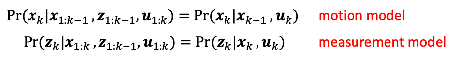
where:

• the latter is much simpler, but of course has a computation and accuracy trade-off.

• and again, knowing either of the two (especially the first one) will be very useful to update your belief estimates

Motion Models

A motion model basically is a transition model that can be applied to update your belief distribution:

If we have a belief distribution over $\mathbf{x}{k-1}$, the motion model $\Pr[ \mathbf{x}{k} \vert \mathbf{x}{k-1}, \mathbf{u}{k}]$ describes how you should then update your belief distribution given an action $\mathbf{u}_k$.

For example, even given a simple motion, you might have a distribution of where your robot is actually at.

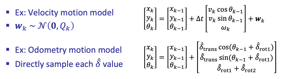
Velocity Motion Model

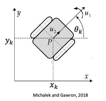
One way to describe how this transition works is by velocity vectors. Given velocity controls, e.g., $\mathbf{u} = (w, \vec{v})$ in the following example

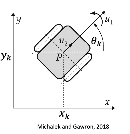
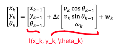
you can then model the transition function as:

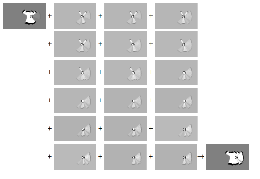
\[\begin{bmatrix} x_k \\ y_k \\ \theta_k \end{bmatrix} = \begin{bmatrix} x_{k-1} \\ y_{k-1} \\ \theta_{k-1} \end{bmatrix} + \underbrace{\Delta t \begin{bmatrix} v_k \cos \theta_{k-1} \\ v_k \sin \theta_{k-1} \\ \omega_k \\ \end{bmatrix} + \mathbf{w}_k}_{\text{your model's design}}\]

where the probabilistic part comes in by how we model the error vector $\mathbf{w}_k$. If we have no prior about it:

• a multivariate Gaussian with zero mean vector, but some non-zero covariance (which you need to define)

• then how you design this covariance matrix changes what the state distribution looks like:

  

• or if you really have no idea, this can also be estimated by some machine learning model + some data

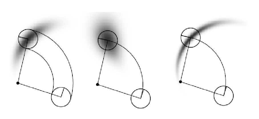
Odometry Motion Model

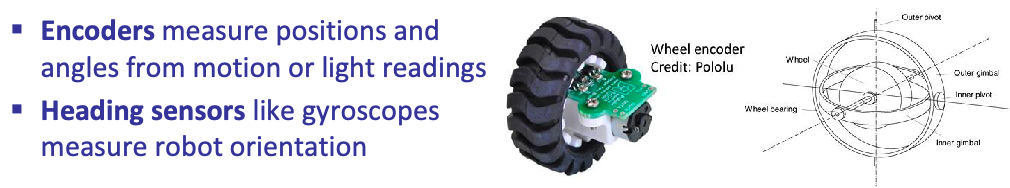
Another common motion model is based on odometry measurment, typically when you have wheel encoder.

Given three “controls” $\delta_{rot1}$, $\delta_{trans}$, $\delta_{rot2}$ being initial rotation, translation, and final rotation:

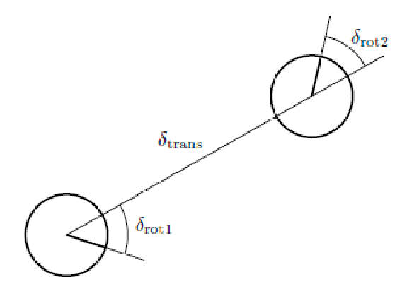
You can then model transition being

\[\begin{bmatrix} x_k \\ y_k \\ \theta_k \end{bmatrix} = \begin{bmatrix} x_{k-1} \\ y_{k-1} \\ \theta_{k-1} \end{bmatrix} + \begin{bmatrix} \hat{\delta}_{trans} \cos(\theta_{k-1} + \hat{\delta}_{rot1}) \\ \hat{\delta}_{trans} \sin(\theta_{k-1} + \hat{\delta}_{rot1}) \\ \hat{\delta}_{rot1} + \hat{\delta}_{rot2} \end{bmatrix}\]

where $\hat{\delta}$ are the true rotation/translation + some noise vector.

Measurement Models

Measurement models describe how sensor measurements are generated. These can also have noises due to stuff like misreadings, unexpected objects, etc. Therefore, the goal is how to represent the “real measurement” (i.e. what you really saw) probabilistically!

Maps and Range Finders

In this section, we have measurements are often described relative to some map

A map is an environment where you basically know a priori where is the obstacles/the free space of the robot.

One simple way to obtain measurement in this case is using range finders

A range finder measure range and/or bearing to fixed landmarks (or obstacles) in the environment.

For example, the map and beams shot out by some range finder is shown below:

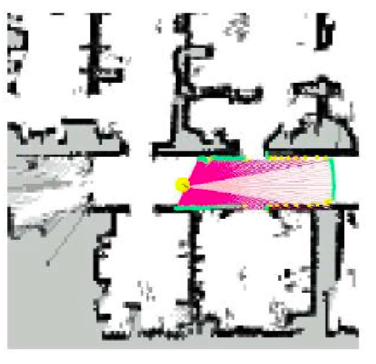
so how would you model measurements in this case?

Landmark Measurement Model

Then, we can model “measurements” as the position of the obstacles given the location of the current robot. This is also called a landmark measurement model.

note that here we ignored measurements that we could “collect from the range finder” here. In practice, you could combine the results from this measurement model with actual measurements.

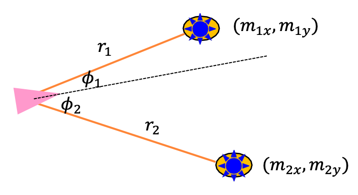
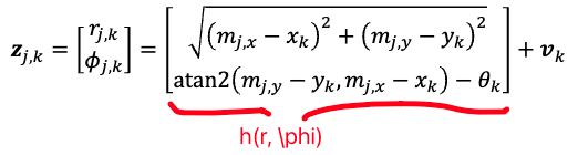
Then the measurement model for each landmark $j$​ at step $k$ of the robot is given by

\[\mathbf{z}_{j,k} = \begin{bmatrix} r_{j,k}\\ \phi_{j,k} \end{bmatrix} = \begin{bmatrix} \sqrt{(m_{j,x} - x_k)^2 + (m_{j,x} - y_k)^2}\\ \text{atan2}(m_{j,y} - y_k, m_{j,x} - x_k) - \theta_k \end{bmatrix} + \mathbf{v}_k\]

so your full measurement would just be:

\[\mathbf{z}_k = \{ \mathbf{z}_{1, k}, \mathbf{z}_{2, k}, ...,\mathbf{z}_{n, k} \}\]

where:

• the $-\theta_k$​ appears is because the robot has its own orientation

• $\mathbf{v}_k$ will be measuring the error

Localization

Finally, to figure out measurement above, you first need to figure out where the robot is relative to the map.

Localization is the problem of determining a mobile robot’s pose (position and orientation) or its coordinate transformation relative to a known map

An example of a hard global localization problem: kidnapped robot problem (your robot suddenly transported to a new location). This task can be used as a measure of how good your localization algorithm is.

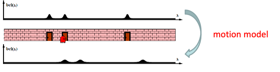
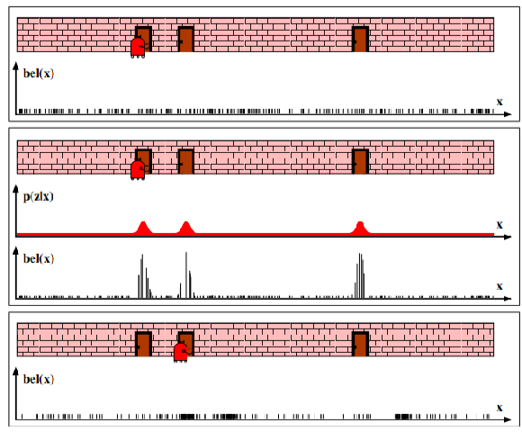
In general, an example of localization would look like:

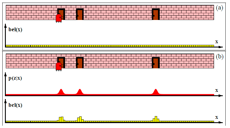
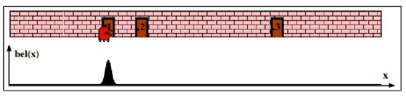
1. consider a 1-D robot, where you don’t really know where your robot is, except that its near a door.

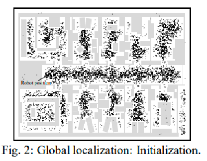
2. At the beginning, since you have no idea where you are, your initial belief state estimate would be uniform:

   

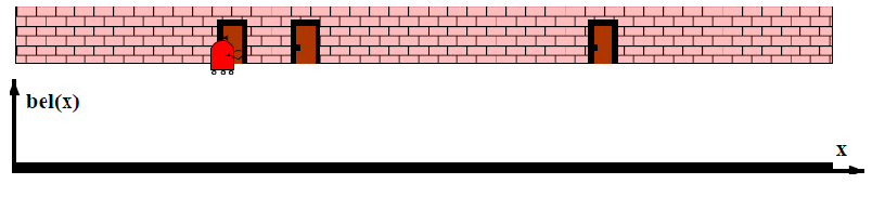
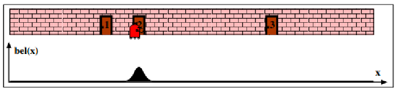
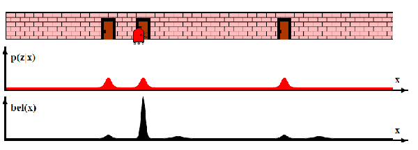
3. But you can measure the location of the door as a function of $x$​ (i.e., with a measurement model). Since you see three doors, you can then update your estimate being your robot near any of one of the three door:

   

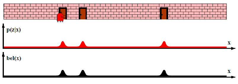
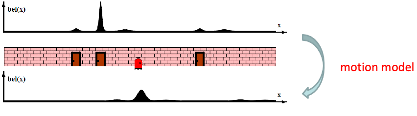
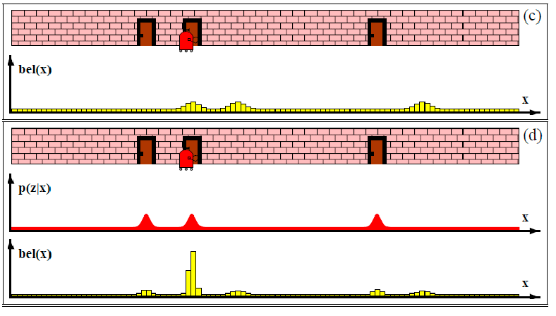
4. Then, let’s say you moved your robot a bit. You can then update your belief again using a motion/transition model:

   

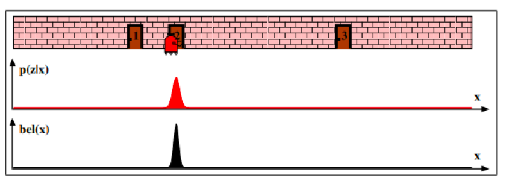
5. After that, say you make another measurement and found that you are still at a door. Then you have quite some good estimate of where your robot is:

   

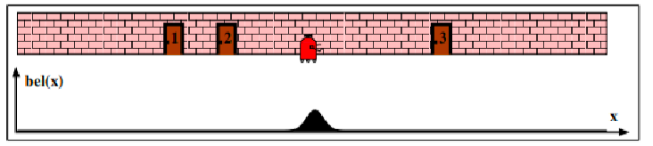
6. Lastly, if you move your robot again, your belief state estimate would be more confident:

   

Bayes Filters and Grid Localization

Now, we can formally define how to get from:

\[B(\mathbf{x}_k) = p( \mathbf{x}_k|\mathbf{z}_{1:k},\mathbf{u}_{1:k} ) \to B(\mathbf{x}_{k+1})= p( \mathbf{x}_{k+1}|\mathbf{z}_{1:k+1},\mathbf{u}_{1:k+1} )\]

with a bit more detail, we will see this being:

• given some movement $\mathbf{u}{k+1}$, use motion model to predict the next state $B(\mathbf{x}{k}) \to B’(\mathbf{x}_{k+1})$
• given some measurement $\mathbf{z}{k+1}$, use measurement model to predict the next state $B’(\mathbf{x}{k+1}) \to B(\mathbf{x}_{k+1})$

Bayesian Inference

Recall that bayes theorem shows:

\[p(x_i | x_j) = \frac{p(x_j | x_i)p(x_i)}{p(x_j)}\]

the practical usage of this is basically in inferences:

\[\text{posterior} = \frac{\text{likelihood} \times \text{prior}}{\text{normalization constant}}\]

and that this holds with multiple terms

\[p(x_i | x_j, y_1, ..., y_m) = \frac{p(x_j|x_i, y_1,..,y_m)p(x_i| y_1,..,y_m)}{p(x_j|y_1,..,y_m)}\]

where basically the original equation holds if we condition every term additionally on $y_1,..,y_m$.

So how can we use it?

Bayes Filter

Consider a simplified case we we have a prior belief $B=p(\mathbf{x}{k-1})$ and a transition model $p(\mathbf{x}{k}\vert \mathbf{x}_{k-1})$, assuming no control:

\[p(\mathbf{x}_{k}) = \int p(\mathbf{x}_{k}|\mathbf{x}_{k-1}) p(\mathbf{x}_{k-1}) d\mathbf{x}_{k-1}\]

but now suppose we observed something, i.e. have a measurement model $p(\mathbf{z}{k}\vert \mathbf{x}{k})$

\[p(\mathbf{x}_{k}|\mathbf{z}_{k}) = \frac{p(\mathbf{z}_{k}|\mathbf{x}_{k})p(\mathbf{x}_{k})}{p(\mathbf{z}_{k})} = \eta^{-1}p(\mathbf{z}_{k}|\mathbf{x}_{k})p(\mathbf{x}_{k})\]

where here is where the bayes theorem come in:

• $\eta$​​ can be computed afterwards to normalize everything to 1.0
• $p(\mathbf{x}_{k})$​ is computed from the previous step.

This means to get actually get from $B(\mathbf{x}_k) \to B(\mathbf{x}_{k+1})$ we will take two steps:

• motion prediction: given that we took an action:
  1. previous belief $B(\mathbf{x}{k-1} ) = p(\mathbf{x}{k-1}\vert \mathbf{z}{1:k-1},\mathbf{u}{1:k-1})$
  2. given an action the robot took $\mathbf{u}_k$
  3. we want to compute a motion model update for the belief states $B’(\mathbf{x}{k} ) = p(\mathbf{x}{k-1}\vert \mathbf{z}{1:k-1},\mathbf{u}{1:k})$ ​

  to be more specific, we show that:

  

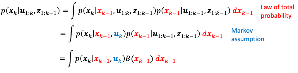
  where this basically says:

  \[B'(\mathbf{x}_{k}) = \int \underbrace{p(\mathbf{x}_{k}|\mathbf{x}_{k-1}, \mathbf{u}_{k})}_{\text{motion model}} B(\mathbf{x}_{k-1}) d\mathbf{x}_{k-1}\]
• obversation update: we then make a measurement and further refine our belief state estimate:
  1. given $B’(\mathbf{x}{k} ) = p(\mathbf{x}{k-1}\vert \mathbf{z}{1:k-1},\mathbf{u}{1:k})$
  2. given an observation $\mathbf{z}_k$
  3. we want to compute a measurement model update/final update for the belief states $B(\mathbf{x}{k} ) = p(\mathbf{x}{k}\vert \mathbf{z}{1:k},\mathbf{u}{1:k})$ ​

  to be more specific, we show that:

  

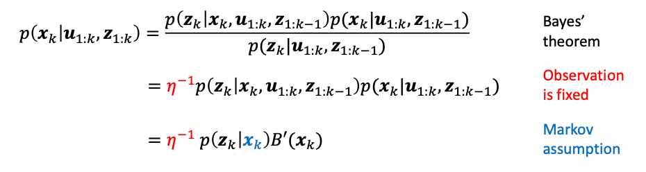
  where in the first equality, we split $\mathbf{z}{1:k} = \mathbf{z}{k}, \mathbf{z}_{1:k-1}$ and this bayes theorem is apparent. This therefore says

  \[B(\mathbf{x}_{k}) = \eta^{-1} \underbrace{p(\mathbf{z}_{k}|\mathbf{x}_{k}, \mathbf{u}_{k})}_{\text{measurement model}} B'(\mathbf{x}_{k})\]

  and depending on how your insert your assumption, you measurement model could even be:

  \[p(\mathbf{z}_{k}|\mathbf{x}_{k}, \mathbf{u}_{k}) \iff p(\mathbf{z}_{k}|\mathbf{x}_{k})\]

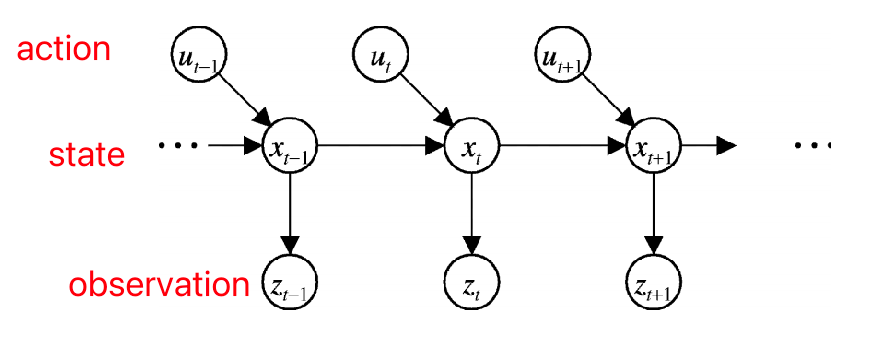
Visually, its like we are doing an HMM update

This means, in summary:

Bayes Filter: the exact computation of $B(\mathbf{x}_{k})$ where:

1. given a prior belief $B(\mathbf{x}{k-1})$= $p(\mathbf{x}{k-1}\vert \mathbf{z}{1:k-1},\mathbf{u}{1:k-1})$
2. given a robot motion $\mathbf{u}_k$, update the belief:

\[B'(\mathbf{x}_{k}) = \int p(\mathbf{x}_{k}|\mathbf{x}_{k-1}, \mathbf{u}_{k}) B(\mathbf{x}_{k-1}) d\mathbf{x}_{k-1}\]

1. given a measurement $\mathbf{z}_k$, update the belief:

\[B(\mathbf{x}_{k}) = \eta^{-1} p(\mathbf{z}_{k}|\mathbf{x}_{k}, \mathbf{u}_{k}) B'(\mathbf{x}_{k})\]

where sometimes you could also see $p(\mathbf{z}{k}\vert \mathbf{x}{k}, \mathbf{u}{k}) \iff p(\mathbf{z}{k}\vert \mathbf{x}_{k})$ being interchangeable.

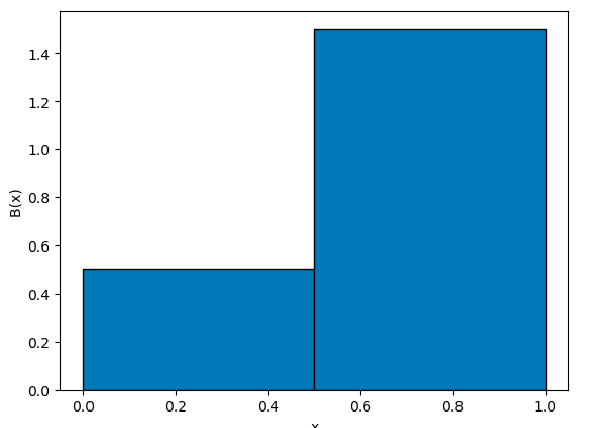
For example, suppose we have a 1D robot that moves between $[0,1]$ and we have a prior belief:

\[B(x_{k-1}) = 2x_{k-1}, \quad 0 \le x_{k-1} \le 1\]

Visually, this means the we think the robot is

Then:

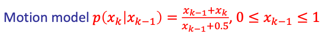
• motion model update: let a motion model be given, being:

  \[p(x_{k} | x_{k-1}) = \frac{x_{k-1} + x_k}{x_{k-1} + 0.5},\quad 0 \le x_k \le 1\]

  plugging in the equation, we get:

  \[B'(x_k) = \int_0^{1} \frac{x_{k-1} + x_k}{x_{k-1} + 0.5} 2x_{k-1} dx_{k-1} = x_{k} (2 - \ln 3) + 0.5 \ln 3,\quad 0 \le x_k \le 1\]

  where:

  • the information of how the robot moved is embedded in the motion model/transition model
  • this motion model says: given the robot moved a bit, I can estimate the chances that now I am in a position $x_k$ given I was previously at $x_{k-1}$.
  • therefore, to visualize the motion model, it will be a 2D surface.

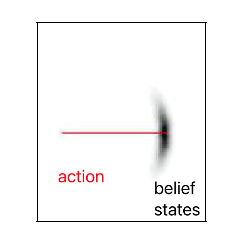
  but this $B’$ can be visualized as:

  

  which indicates the movement is probably to the left.

• measurement model update: let a measurement model be given, being:

  \[p(z_k | x_k) = 1, \quad 0.5 \le x_k \le 1\]

  plugging in the equation, we get:

  \[B(x_k) = \eta^{-1} p(z_k | x_k) B'(x_k) = \eta^{-1} (x_k (2 - \ln 3) + 0.5 \ln 3), \quad 0.5 \le x_k \le 1\]

  where:

  • again, the information of what you measured is embedded in the measurement model
  • this essentially measures the likelihood of the robot being at $x_k$ given what you just observed.

  this final $B$ can be visualized as:

  

This gives me a full updated $B(x_k)$​​ after a movement and a measurement.

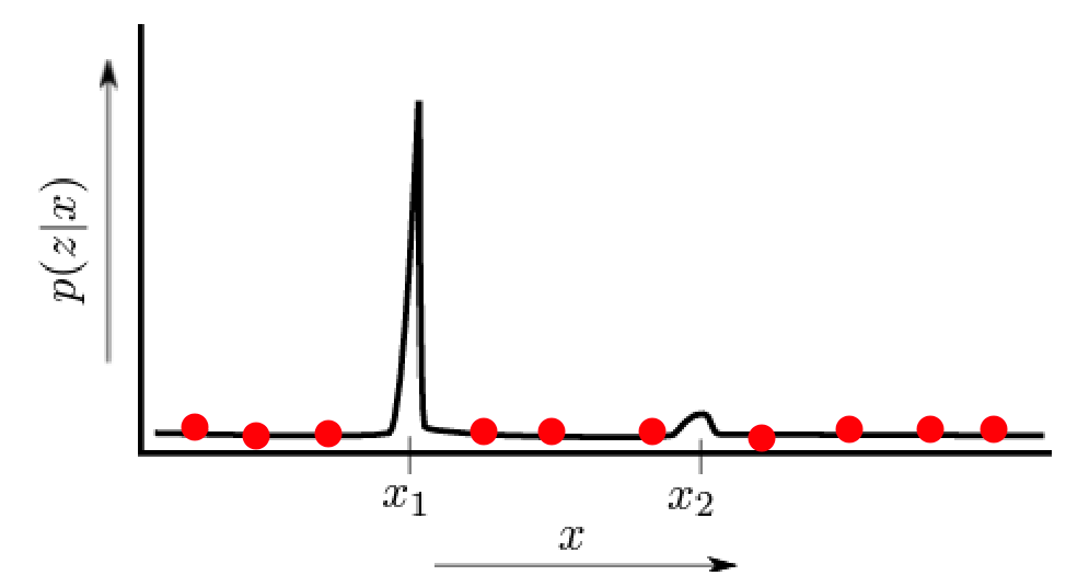
Histogram Filters

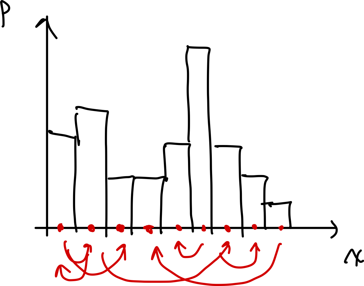
Idea: this integration over motion model would be computationally expensive and near intractable at high dimensional space. But we can discretize over the state space (e.g., grid state space) and do sum instead.

so we can have:

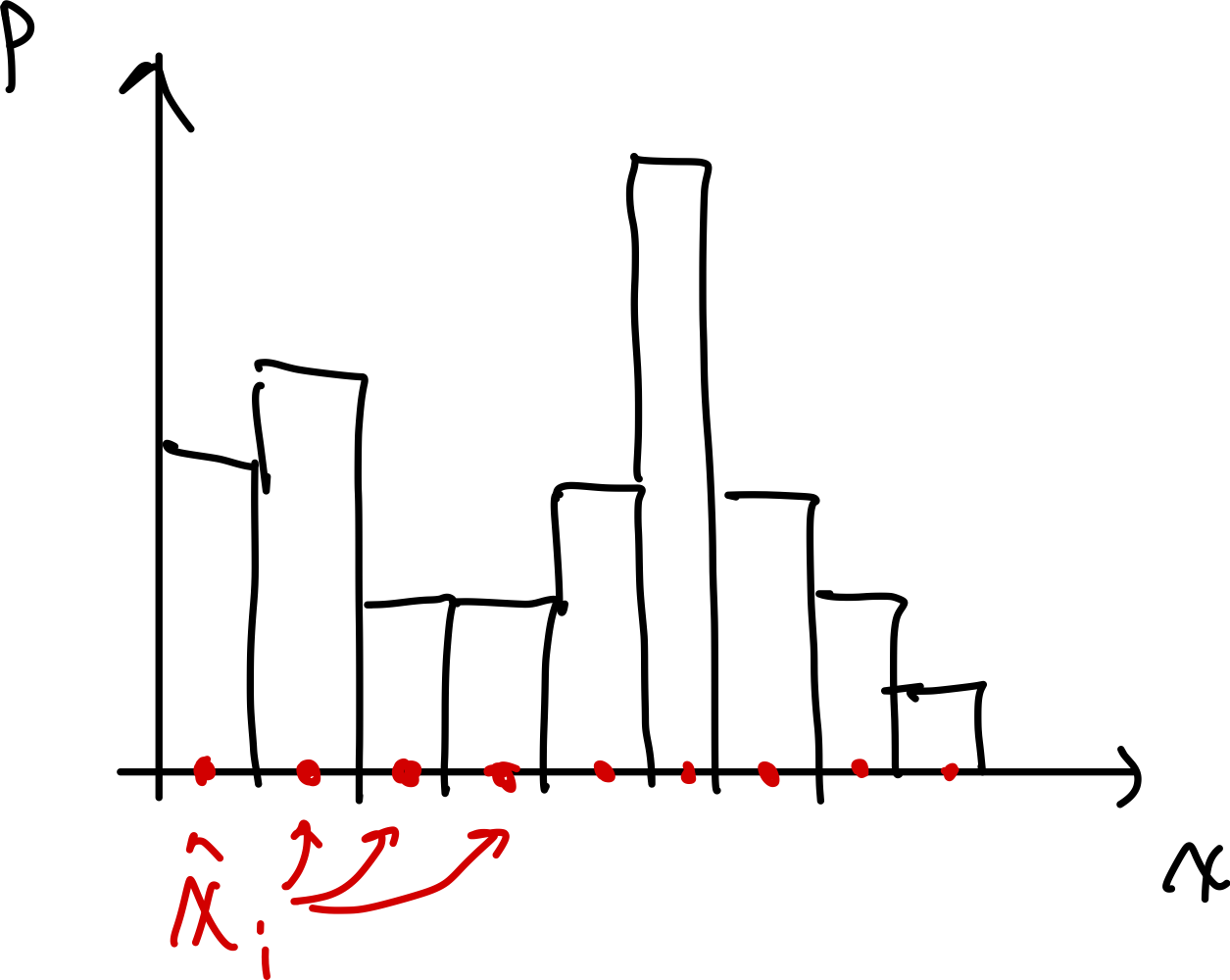
• chunk a continuous space into grid regions $x_i$
• every position in a grid region $x_i$ will have the same probability $p_i$ (e.g. probability of the mean coordinate $\hat{x}_i$)

Visually, the red dots are the representative state $\hat{x}_i$ we use for $p_i$

Then we have

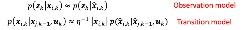
where the $\vert x_{i,k}\vert$ describes the volume of that grid region $x_i$​. The transition/motion model is then:

For example:

Continuous Transformations	Discrete Transformations

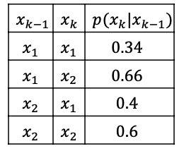
More concretely, consider discretizing our example in the previous section. Let’s still have $B(x_{k-1}) = 2x_{k-1}$ into two bins:

so basically we have two representative points: $x_1=0.25,x_2=0.75$. Then our discretized motion model looks like

Full Motion Model	Discretized (NxN matrix)

Hence our belief update $B’(x_k)$ becomes a discrete sum:

\[B'(\mathbf{x}_{k}) = \sum_{\mathbf{x}_{k-1}} p(\mathbf{x}_{k}|\mathbf{x}_{k-1}) B(\mathbf{x}_{k-1})\]

So we get:

\[B'(x_k) = \begin{bmatrix} B'(x_k=0.25) \\ B'(x_k=0.75) \end{bmatrix} = \begin{bmatrix} 0.34 (0.5) + 0.4 (1.5) \\ 0.66 (0.5) + 0.6(1.5) \end{bmatrix} = \begin{bmatrix} 0.77 \\ 1.23 \end{bmatrix}\]

and finally applying the measurement model $p(z_k\vert x_k)=1$ for $0.5\le x_k\le1$:

\[B(x_k) = \eta^{-1} p(z_k|x_k)B'(x_k) = \eta^{-1} \begin{bmatrix} 0.0 \\ 1.23 \end{bmatrix} = \begin{bmatrix} 0.0 \\ 2.0 \end{bmatrix}\]

which zeroed out the first cell entirely.

Histogram Filter: the approximate computation of $B(\mathbf{x}_{k})$ where after we discretized all states:

1. given a discretized belief $B(\hat{\mathbf{x}}{k-1})$= $p(\hat{\mathbf{x}}{k-1}\vert \mathbf{z}{1:k-1},\mathbf{u}{1:k-1})$
2. given a robot motion $\mathbf{u}_k$, update the belief:

\[B'(\hat{\mathbf{x}}_{k}) = \sum_{\hat{\mathbf{x}}_{k-1}} p(\hat{\mathbf{x}}_{k}|\hat{\mathbf{x}}_{k-1}, \mathbf{u}_{k}) B(\hat{\mathbf{x}}_{k-1})\]

1. given a measurement $\mathbf{z}_k$, update the belief:

\[B(\hat{\mathbf{x}}_{k}) = \eta^{-1} p(\mathbf{z}_{k}|\hat{\mathbf{x}}_{k}, \mathbf{u}_{k}) B'(\hat{\mathbf{x}}_{k})\]

where $p(\hat{\mathbf{x}}{k}\vert \hat{\mathbf{x}}{k-1}, \mathbf{u}{k})$ and $p(\mathbf{z}{k}\vert \hat{\mathbf{x}}{k}, \mathbf{u}{k})$ are the discretized motion and measurement models (i.e., they becomes a $N \times N$ matrix instead of a continuous function, if you have $N$ discretized states)

Grid Localization

As a visual example, we can apply this discretization method to the Localization problem. The difference is that here we discretized the states but assume that the measurement/motion model given was still at full resolution (i.e., continuous).

Given the first measurement:

after taking an action (to the right) and another measurement

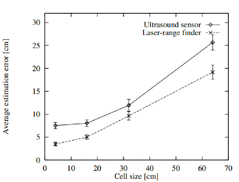
Grid Resolution

One problem of discretizatoin is that you lose information within a cell. So there is now a trade-off.

A few practical solutions to mitigate this:

• Topological grid: Regions are defined based on features and “significant” locations in the environment
• Metric grid: Regions are fine-grained cells of uniform size

Of course, we can plot the errors as a function of grid size (higher size = coarser)

But other interesting methods include:

• Increase the amount of noise that is assumed by the model. This is a bit counter-intuitive:
  • With coarse resolutions, the motion and measurement models may vary a lot within grid cells
  • so we now model that variation by making the models less accurate
• tricks to make computation faster:
  • ensor subsampling (e.g., using a subset of measurements)
  • delayed motion updates

Dynamic Decomposition

In practice, robot will not move very far within a short number of steps. So we will uslaly see zero probability (white) in most parts.

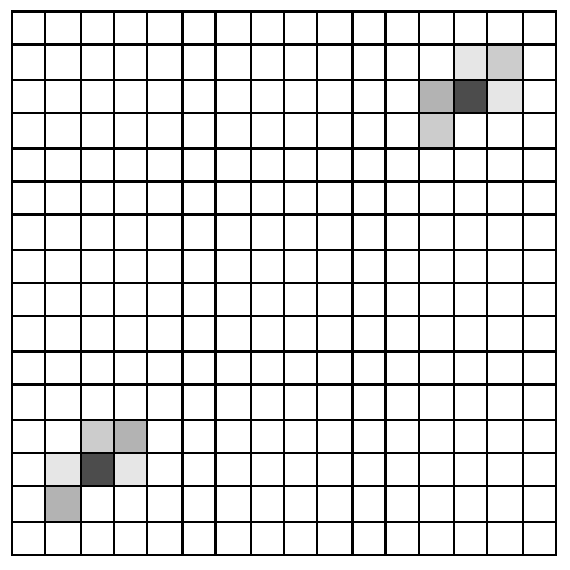
Idea: a dynamic decomposition then varies resolution in different regions

• merge regions with similar or low probabilities
• split regions where probability is higher for better representation

Visually:

Particle Filters and MC Localization

Instead of grids to do discretization, we can use random samples (I.e., particles)

Particle Filters

Alike using grid to represent distributions, you can just use particles to also do discretization

BUt why would this be useful? Consider you have:

• a prior belief $B(\mathbf{x}_0)$
• consider $M$ state particles (i.e., “clones” of your robot) being $(\mathbf{x}^1_0, \mathbf{x}^2_0, …, \mathbf{x}^M_0)$

Then, finding $B(\mathbf{x}_1)$ means:

Particle Filter: estimate $B(\mathbf{x}_{k+1})$ by imaging clones/hypothesis of your robot sampled from $B(\mathbf{x}_k)$, then do the motion/measurement model update to each of these particles.

For each timestep $k$:

1. for each particle $j$:
   • motion update: sample new particle $\mathbf{x}^j_{k+1}$ from $p(\mathbf{x}_{k+1}\vert \mathbf{x}^j_k, \mathbf{u}_k)$
   • measurement update: adjust the weight of the particle $w^j_{k+1} = p(\mathbf{z}{k+1}\vert \mathbf{x}^j{k+1})$
2. resample particles from the distribution of the weights $(w_{k+1}^{1}, w_{k+1}^{2}, …, w_{k+1}^{M})$

\[B(\mathbf{x}_{k+1}) = \text{density of the resampled particles}\]

implementation-wise this is basically sampling particles with repetition at $\mathbf{x}^j_{k+1}$ again, but with new weights

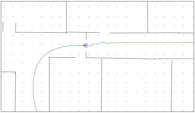
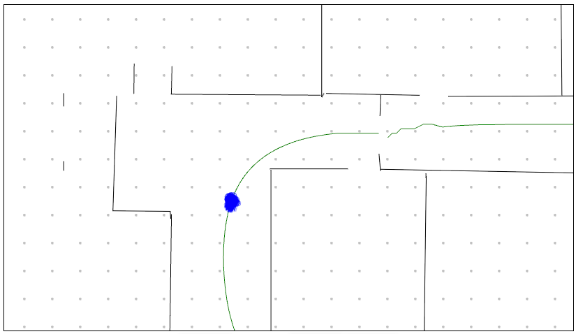
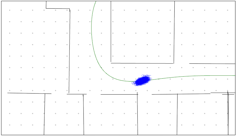
Monte Carlo Localization

An example of usage of particle filters is do localization. Since essentially this distribution is like the evolution of each particle, this is also called Monte Carlo Localization.

now, each particle has a weight defined by the measurement model (the second row).

Motion Model Sampling

Recall that the motion model defines a probability distribution to transform from one state to another. So how do we model each particle’s next state?

In the view that each particle is a “clone” of the robot, motion model update is like applying the motion model on that particle plus some noise. For example:

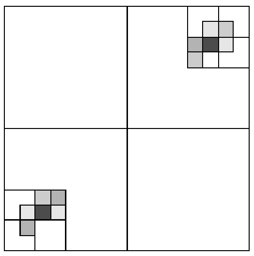
but in general, if your motion model is some crazy weird distribution, you can do rejection sampling to have new samples at a likely part of this distribution

Rejection Sampling as a way to apply motion model to particles. Given a particle $\mathbf{x}_{k-1}^{j}$ and a motion $\mathbf{u}_k$:

1. Sample one new particle $\mathbf{x}{k}$ on the support (non-zero region) of the motion model $p(\mathbf{x}{k}\vert \mathbf{x}_{k-1}^{j}, \mathbf{u}_k)$
2. Uniformly sampling $c$ between $0$ and $\max p(\mathbf{x}{k}\vert \mathbf{x}{k-1}^{j}, \mathbf{u}_k)$
3. if this particle has probability $p(\mathbf{x}{k}\vert \mathbf{x}{k-1}^{j}, \mathbf{u}_k) > c$, then accept this particle as the new state. Otherwise, reject it and repeat the process.

the idea is that you are sampling from the motion model but rejecting samples that are unlikely.

Visually, suppose $f(x)$ is your motion model given your previous particle, and you sampled $x$ for the first time, and $x’$ the next:

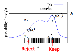
So you basically got $x’$ as your particle’s next state.

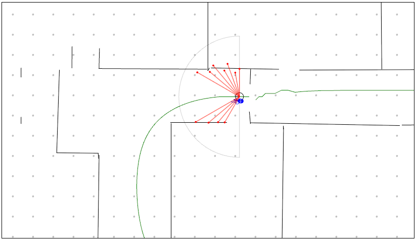
Measurement Model LIkelihood

Recall that measurement model defines a probability distribution to get a measurement given the state. So how do we model each particle’s new probability/likelihood/weight given some measurement?

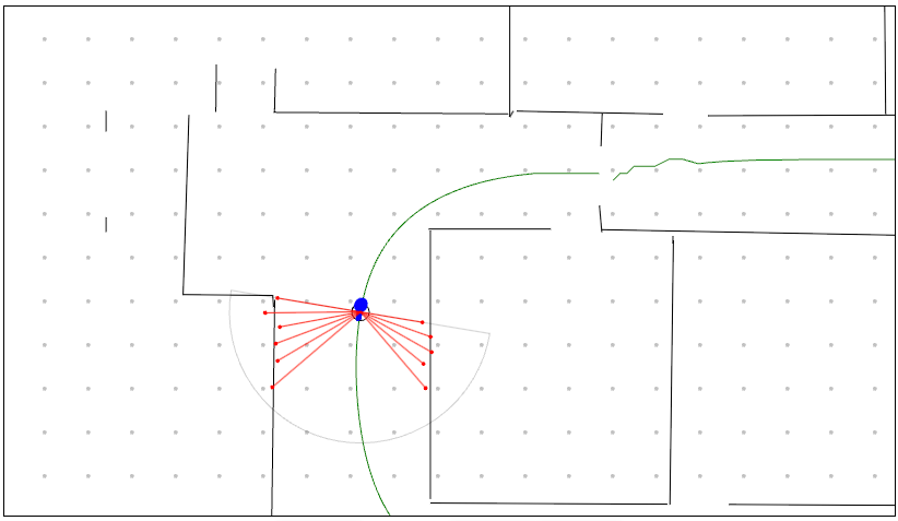
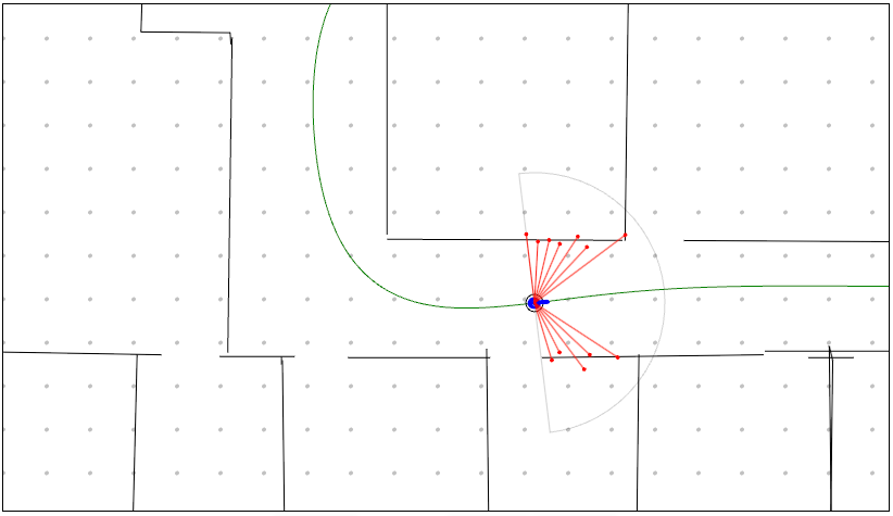
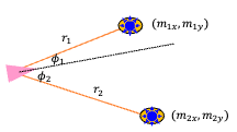
Consider an example where measurements are from range finders:

where the measurement model for each landmark $l$​ at step $k$ of the robot is given by

\[\mathbf{z}_{l,k} = \begin{bmatrix} r_{l,k}\\ \phi_{l,k} \end{bmatrix} = \begin{bmatrix} \sqrt{(m_{l,x} - x_k)^2 + (m_{l,x} - y_k)^2}\\ \text{atan2}(m_{l,y} - y_k, m_{l,x} - x_k) - \theta_k \end{bmatrix} + \mathbf{v}_k\]

Then, we can use this to specify the probability of a particle seeing the measurements as a normal distribution:

\[\mathcal{N}(\mathbf{z}_k, R)\]

given some specified covariance matrix $R$. Visually, say for particle $j$, it should see obstacle $l$ at $r=\hat{r}l^{j}$ (computed using the $r{l,k}$ equation):

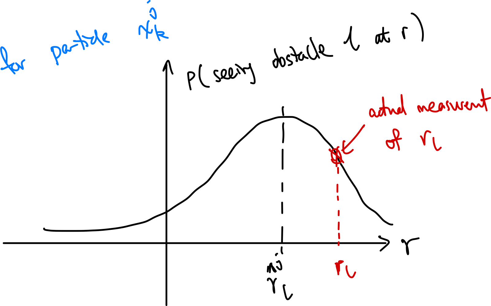
This means you can then compute the likelihood of seeing the measurement by indexing the actual measurement $\mathbf{z}_k$ from the above probability distribution. This is used as the likelihood/weight of this particle.

Importance Sampling and Resampling New Particles

Recall that the final step of the particle filter is to resample new particles from the existing particles but with these weights from the measurement model. Why and how do we do this?

First, we discuss why.

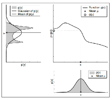
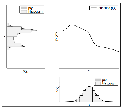
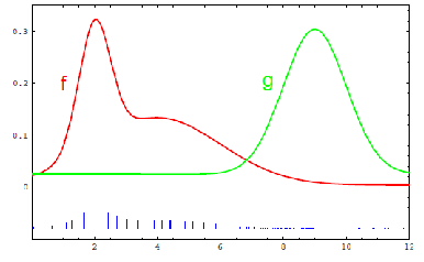
Recall the goal of particle filters is to approximate the true distribution $B(\mathbf{x}_k)$ with particles. But our initial particles are sampled from a distribution $B’(\mathbf{x}_k)$ that is different from the true distribution. As you may have guessed, this means to mimic these particles to be sampled from the true distribution, we need to do importance sampling:

1. suppose we sampled particles from $g$, but we wanted to sample from $f$:

   

2. (see the RL notes for proof) you can show that for any function $h(x)$:

   \[\mathbb{E}_{x \sim f}[h(x)] = \mathbb{E}_{x \sim g}\left[\frac{f(x)}{g(x)}h(x)\right]\]

   so that you can adjust the weights of the particles to be from the true distribution.

   

   and these importance weights corresponds to the weight computed from the measurement model.

3. Therefore, to mimic the true distribution, we finally resample particles from the distribution of the weights $(w_{k+1}^{1}, w_{k+1}^{2}, …, w_{k+1}^{M})$ for each particle. (This means that we won't have new states, but just redistribute them with repetition to better represent the true distribution)

Implementation-wise, to resample new particles:

• the resampling weights are the $p(z_k \vert x_k^j)$ being the likelihood of seeing $z_k$ if the robot is at this particle

• the resampling step aims to change the distribution from $B’(x_k)$ to $B(x_k)$ by:

  • changes the weight of the particles

    

  • resample (with repetition) from the distribution above

Example: Particle Filter Updates

Consider a uniform unitialization of particle filters:

Given some oberservation, many of these particles (hypothesis) disappear:

Less lucky	If you are lucky

More visually (see Interactive Robotics Algorithms (utexas.edu) for more examples)

• without measurement and only uses motion model = over time error accumulates and particles spread out

Step 0	Step 100	Step 200

• with measurement weights = density will be more certain as the robot moves around

Step 0	Step 100	Step 200

Sampling Variance

Pros for particle filters

• Easy to implement, accuracy increase with number of particles
• Nonparametric: can easily represent complex distributions

Cons:

• need enough particles: too few samples gives strong biases
• you may have a high sampling variance (estimated distribution may be very difference across runs)

Reducing Variance

You can deal with bias by adding particles, but what about variance?

• reduce the frequency of resampling (more deterministic)

  • For example, we should not resample if we know that state is static
  • or determine when to resample can be based on variance of likelihood weights
    • When weight variance is low and weights have similar values, not needed
    • When weight variance is high and weights have very different values, resampling can shift particles away from low weight regions

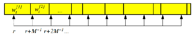
• Low-Variance Sampling: Common random number or correlated sampling are sampling methods that are near deterministic.

  • e.g.,: sample the first particle with $\text{rand}(0, M^{-1})$, and the rest $M-1$ samples deterministically at intervals of $M^{-1}$

  • visually, the particle picked is actually still obeying the probability distribution (small bins have no arrows!)

    

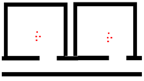
Particle Deprivation

Since your particles are eventually converging (not sampling at new locations), this may be problematic. In fact, because re-sampling is a random process. Suppose you have a robot where it didn’t move and all measurements are identical. Then you would see:

Initial	Over time

so due to randomness:

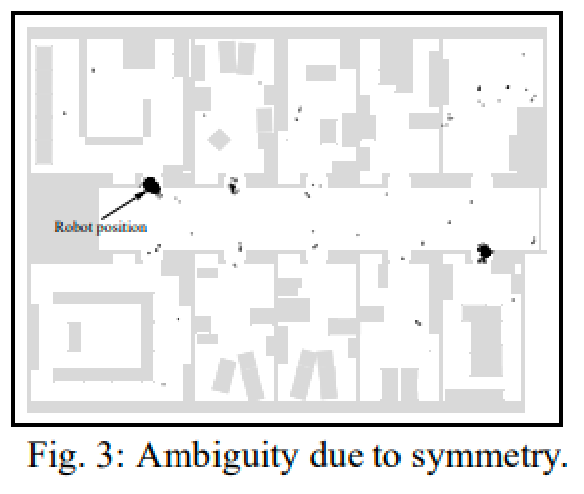
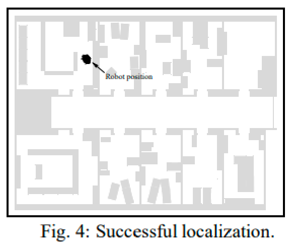
• resampling will eventually cause all particles to converge toward one of the states. But this is wrong—we should still have a uniform belief!
• in fact, it will also happen to the kidnapped robot problem. (particle filter is unable to correct itself when the robot’s state has changed drastically, see next section for an example)

Distribution Mismatch

Your samples might not really match the real distribution if your target distribution is very different. For example, the actual distribution may look like the dark line

then no matter how you do importance sampling adjustment, there is no hope. To address this issue we can consider Random Particle Injection.

Random Particle Injection: to address distribution mismatch, we can randomly inject new particles at each iteration.

At each iteration of the particle filter:

1. additionally compute two moving averages of the particles: one with a short window $w_s$ and one with a long window $w_l$
2. modify the resampling prodcedure to:
   • only with probability $\min(1, \frac{w_s}{w_l})$ resample the particles
   • otherwise replace the particle with a completely random one

The intuition is that when $w_{s} \ll w_l$, it means that the particles are converging and we should inject new randomness (alike exploration v.s. exploitation in RL).

Kalman Filters

State estimation of continuous distributions and in continuous spaces is generally non-trivial.

Previous section introduced non-parametric methods to estimate $B(\mathbf{x})$ as a distribution. In this section, we show that if you go for parametric methods (e.g. assume its Gaussian or mixture of Gaussian), then in practice the computation for state estimation becomes much easier (only need to consider how the parameters of your distribution change).

Gaussian Filters

Since we only need the mean and variance for Gaussian, this can be very parameter-efficient.

\[\text{provide mean and covariance matrix}: \mathbf{x}_k, P_k\]

then you get an entire distribution:

\[B(\mathbf{x}_k) \gets \mathcal{N}(\mathbf{x}_k, P_k) = \frac{1}{(2\pi)^{n/2} \text{det}(P_k)^{1/2}} \exp\left(-\frac{1}{2}(\mathbf{x}_k - \hat{\mathbf{x}}_k)^T P_k^{-1} (\mathbf{x}_k - \hat{\mathbf{x}}_k)\right)\]

in the case of a single Gaussian, its not so suitable for problems that have multiple hypotheses (e.g., you have two strong prior guesses of where the robot is). However, we will later show that it can be easily extended to mixture of Gaussian.

Discrete-Time Linear Systems

We then further assume that state transformations are linear transformations:

\[\begin{cases} \mathbf{x}_k = F_k \mathbf{x}_{k-1} + G_k \mathbf{u}_k + \mathbf{w}_k, & \text{motion model}\\ \mathbf{z}_k = H_k \mathbf{x}_k + \mathbf{v}_k, & \text{measurement model} \end{cases}\]

where you have:

• $\mathbf{x} \in \mathbb{R}^n$ is the state, $\mathbf{u} \in \mathbb{R}^m$ is the control input, and $\mathbf{z} \in \mathbb{R}^p$ is the measurement
• $F_k$ can be interpreted as a state transition matrix, $G_k$ is the control-input matrix, $H_k$ is the measurement matrix
• $\mathbf{w}_k$ and $\mathbf{v}_k$ are the process and measurement noise, respectively

But why would we be considering linear systems?

In this section, we will (first) focus on linear systems + Gaussian distributions. This is because affine transformations of Gaussian distributions are also Gaussian.

This means that if your prior belief is Gaussian, then the update after applying the motion model and measurement model will also be Gaussian.

At this point you might already be suspicious: Gaussian + affine transformations. Is it practical? The quick peek is that later we will:

• for non-linear transformations, approximate with taylor expansions = linearization
• for non-Gaussian distributions, approximate with mixtures of Gaussian

Kalman Filter Derivation

For discrete-time linear dynamical systems with independent, additive Gaussian noise, the Kalman filter is an optimal, recursive, and closed-form estimator.

• i.e., you can update your belief distribution exactly (as they are parametric)
• i.e., the update can be summarized in closed-form equations with matrix operations

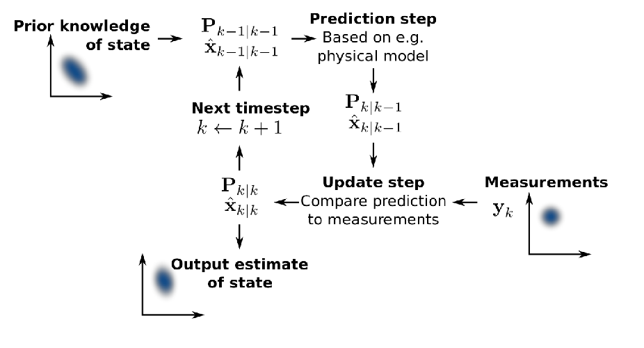
On a high level, the sequence of updates we will do is the same as before:

1. Prediction step: given a prior, make update from motion model

   

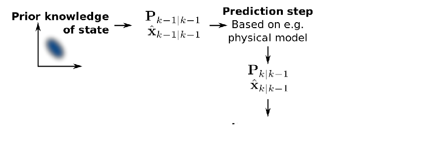
2. Update step: then given measurement model/measurements, refine the belief

   

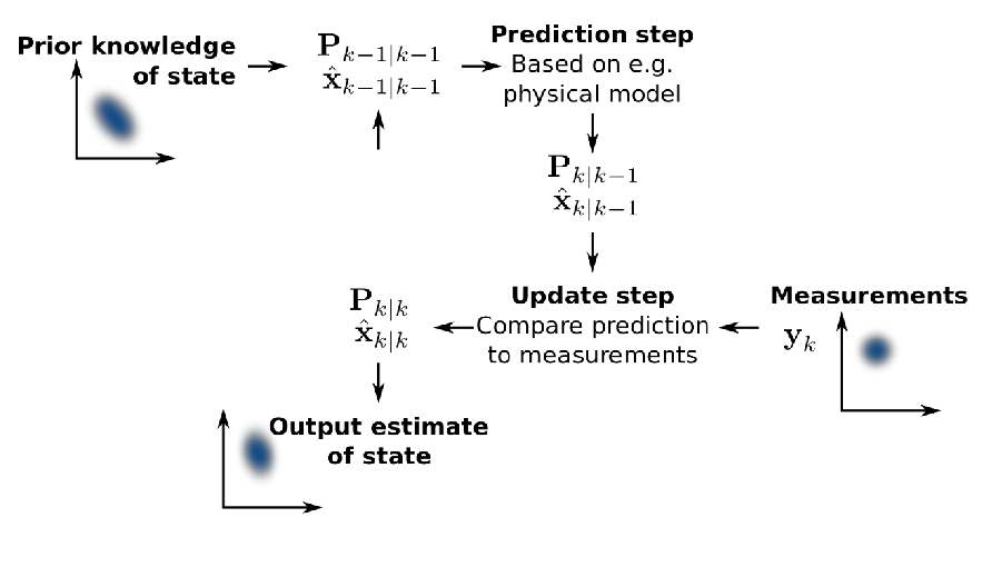
3. Repeat: then repeat the process

   

The only difference from previous methods is that here everything is Gaussian. What does this mean? For example, if your robot moves to the right:

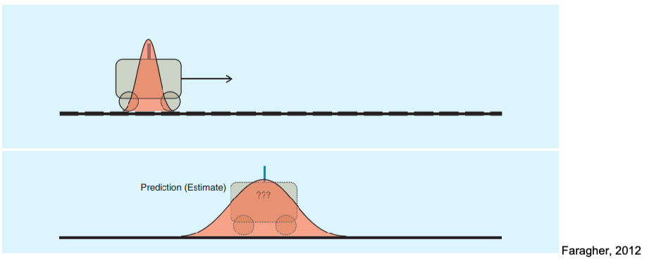
Practically you are just shifting your mean and variance:

• your mean will shift to the right according to the motion model
• your variance variance/uncertainty will increase (i.e., particles spread out as in Particle Filters) if you haven’t seen any measurements

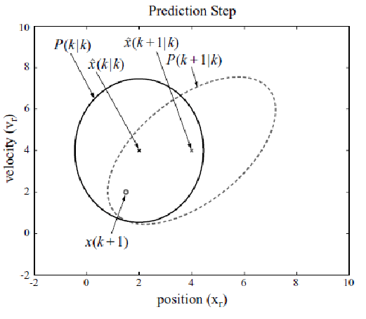
Prediction Step

So how do we update according to the motion model? Suppose we are given a prior Gaussian with known $\hat{\mathbf{x}}{k-1\vert k-1}$ and $P{k-1\vert k-1}$ (e.g., computed from previous iteration):

\[\mathbf{x}_{k-1} \sim \mathcal{N}( \hat{\mathbf{x}}_{k-1|k-1}, P_{k-1|k-1})\]

You now want to do a motion update to figure out your new belief state:

\[\mathbf{x}_{k}' \sim \mathcal{N}( \hat{\mathbf{x}}_{k|k-1}, P_{k|k-1})\]

This turns out to be easy because:

1. if we consider the motion model to be linear:

   \[\mathbf{x}_{k}' = F_{k} \mathbf{x}_{k-1} + G_{k} \mathbf{u}_{k} + \mathbf{w}_{k}, \text{ where } \mathbf{w}_{k} \sim N(0, Q_k)\]

2. then you can derive the new mean and covariance from applying this affine transformation:

   \[\begin{cases} \hat{\mathbf{x}}_{k|k-1} = F_k \hat{\mathbf{x}}_{k-1|k-1} + G_k \mathbf{u}_{k}, & \text{new mean}\\ P_{k|k-1}=F_kP_{k-1|k-1}F_k^T + Q_k, & \text{new variance} \end{cases}\]

   essentially

   • the variance is now “squared”, which intutively corresponds to squring a random variable by $x \to ax$ will square its variance $\sigma^2 \to a^2\sigma^2$​.
   • the mean is just the linear transformation of the previous mean

---

Proof of the covariance update: starting from the definition of covariance matrix:

\[\begin{align*} P_{k|k-1} &= \mathbb{E}[(F_{k} \mathbf{x}_{k-1} + G_{k} \mathbf{u}_{k} + \mathbf{w}_{k})(F_{k} \mathbf{x}_{k-1} + G_{k} \mathbf{u}_{k} + \mathbf{w}_{k})^{T}] - \hat{\mathbf{x}}_{k|k-1} \hat{\mathbf{x}}_{k|k-1}^{T}\\ &= F_{k}( \mathbb{E}( \mathbf{x}_{k-1} \mathbf{x}_{k-1}^{T}) - \hat{\mathbf{x}}_{k-1|k-1} \hat{\mathbf{x}}_{k-1|k-1}^{T}) F_{k}^{T} + \mathbb{E}(\mathbf{w}_{k} \mathbf{w}_{k}^{T}) \\ &= F_{k} P_{k-1|k-1} F_{k}^{T} + Q_{k} \end{align*}\]

where many cross terms disappear in line 2 because $\mathbf{x}{k-1}$ and noise $\mathbf{w}_k$ are independent, hence $\text{Cov}(x{k-1},w_k)=0$.

---

Visually, the mean basically moves exactly like the motion model $F_k$, and then shift the covariance:

Mean Transformation	Covariance Transformation

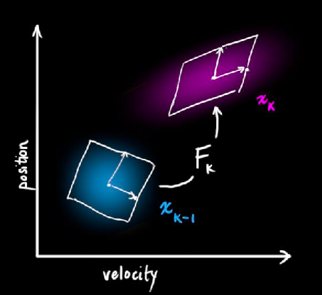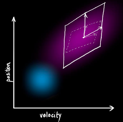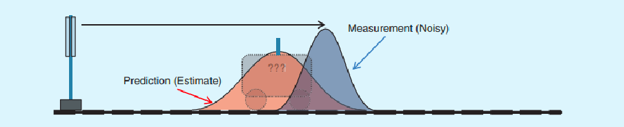
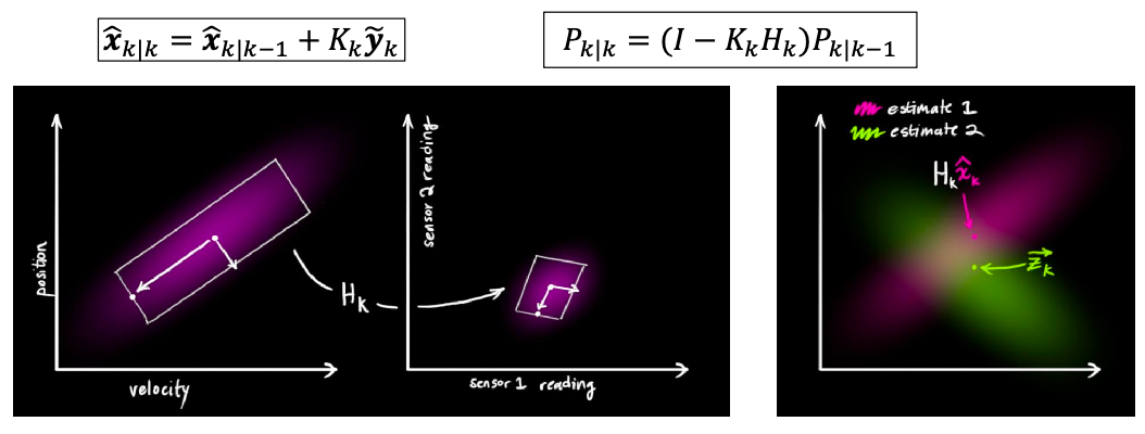
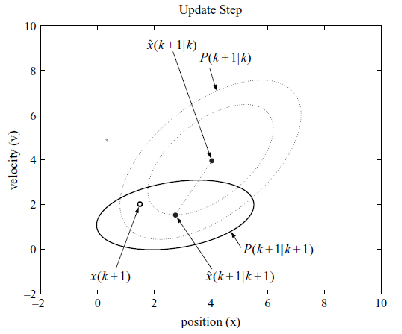
Update Step

Now we have a measurement, and we want to further refine our belief state estimate:

Belief (Orange) and Measurement (Gray)	Belief after Update (Green)

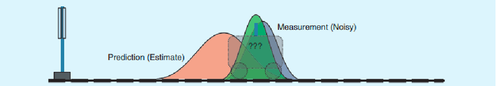so how does it work? This is slightly more complicated.

1. Recall that given a measurement model, the belief state update is given by Bayes’ Theorem:

   \[B(\mathbf{x}_k) = \eta^{-1} p(\mathbf{z}_k|\mathbf{x}_k) B'(\mathbf{x}_k)\]

2. We already have the prior belief after motion model:

   \[\mathbf{x}_{k}' \sim \mathcal{N}(\hat{\mathbf{x}}_{k|k-1}, P_{k|k-1})\]

   and we assumed that transformation is linear:

   \[\mathbf{z}_k = H_k \mathbf{x}_k + \mathbf{v}_k, \text{ where } \mathbf{v}_k \sim \mathcal{N}(0, R_k)\]

3. Then we can first show that given:

   \[\mathbf{z}_k|\mathbf{x}_k' \sim \mathcal{N}(H_k \mathbf{x}_{k}', R_k) = p(\mathbf{z}_k|\mathbf{x}_k')\]

   and finally, because the product of Gaussian is also Gaussian, we can show that the after applying the bayes theorem, the new belief state is also Gaussian:

   \[\begin{cases} \hat{\mathbf{x}}_{k|k} = \hat{\mathbf{x}}_{k|k-1} + K_{k} \tilde{\mathbf{y}}_k, & \text{new mean}\\ P_{k|k} = (I - K_k H_k) P_{k|k-1}, & \text{new variance} \end{cases}\]

   where the additional variables are:

   • $\tilde{\mathbf{y}}k = \mathbf{z}_k - H_k \hat{\mathbf{x}}{k\vert k-1}$ is the error vector or the innovation
   • $K_k = P_{k\vert k-1} H_k^{T}S_k^{-1}$ is the Kalman gain
   • $S_k = H_k P_{k\vert k-1} H_k^{T} + R_k$ is the innovation covariance

   and notice that the only things we need are $P_{k\vert k-1}, P_{k\vert k-1}$ which we know from the previous step, and the constants $H_k, R_k$ from the measurement model.

---

Proof of the mean and variance update: the trick is that because we know the result is a Gaussian, we just have to match the terms:

\[B(\mathbf{x}_k) \propto p(\mathbf{z}_k|\mathbf{x}_k) B'(\mathbf{x}_k) = \exp(- \frac{1}{2} f(\mathbf{x}_k)) \propto \mathcal{N}(\hat{\mathbf{x}}_{k|k}, P_{k|k})\]

Therefore, moving from the LHS we have:

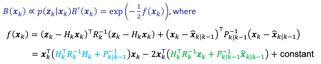
the RHS then is:

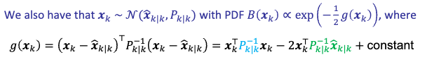
Therefore the green and blue terms have to match, ending up:

\[\begin{cases} P_{k|k}^{-1} = H_k^TR_{k}^{-1}H_k + P_{k|k-1}^{-1}, & \text{new variance}\\ \hat{\mathbf{x}}_{k|k} = P_{k|k} H_k^T R_k^{-1}(z_k - H_k \hat{\mathbf{x}}_{k|k-1}) + \hat{\mathbf{x}}_{k|k-1}, & \text{new mean} \end{cases}\]

To simply them, we can show that:

• using the matrix inversion lemma:

  \[P_{k|k} = (I - K_k H_k) P_{k|k-1}\]

  where $K_k = P_{k\vert k-1} H_k^{T}(H_k P_{k\vert k-1} H_k^{T} + R_k)^{-1}$ is the Kalman gain.

• and the new mean is just a scaled version of the error vector:

  \[\hat{\mathbf{x}}_{k|k} = \hat{\mathbf{x}}_{k|k-1} + K_{k} \tilde{\mathbf{y}}_k\]

  where $\tilde{\mathbf{y}}k = \mathbf{z}_k - H_k \hat{\mathbf{x}}{k\vert k-1}$ is the error vector, or also called the innovation.

Kalman Gain: is a matrix $K_k \in \R^{n \times p}$ governs the amount of correction applied to the belief state

To visualize this, consider we are in the 1D case, such that $K = PH / (H^2P+R)$​. Then given that:

\[P_{k|k} = (I - K_kH_k) P_{k|k-1}\]

• if $P_{k\vert k-1}$ is small, then $K$ is mostly determined by $R$ (the uncertainty from measurement). So the new uncertainty $P_{k\vert k}$ is mostly determined by your measurement.
• if $P_{k\vert k-1}$ is large (previous belief state has large uncertainty), then $K \approx 1/H$​. So new uncertainty is near zero, meaning you just trust the measurement model instead of the previous belief.

Visually:

Summary: Kalman Filter

So in summary, given the previous estimate $\hat{\mathbf{x}}{k-1\vert k-1}$ and $P{k-1\vert k-1}$, the update steps for the mean and covariances look like:

1. Apply motion model:

   \[\begin{cases} \hat{\mathbf{x}}_{k|k-1} = F_k \hat{\mathbf{x}}_{k-1|k-1} + G_k \mathbf{u}_{k}, & \text{new mean}\\ P_{k|k-1}=F_kP_{k-1|k-1}F_k^T + Q_k, & \text{new variance} \end{cases}\]

2. Apply measurement model:

   \[\begin{cases} \hat{\mathbf{x}}_{k|k} = \hat{\mathbf{x}}_{k|k-1} + K_{k} \tilde{\mathbf{y}}_k, & \text{new mean}\\ P_{k|k} = (I - K_k H_k) P_{k|k-1}, & \text{new variance} \end{cases}\]

   where you have:

   • $\tilde{\mathbf{y}}k = \mathbf{z}_k - H_k \hat{\mathbf{x}}{k\vert k-1}$
   • $K_k = P_{k\vert k-1} H_k^{T}S_k^{-1}$
   • $S_k = H_k P_{k\vert k-1} H_k^{T} + R_k$

---

For example, consider a 1D robot with mass $m$ moving in a straight line. Let it have state $\mathbf{x}_k = (x_k, v_k)$ for $x_k$ is the 1D coordinate of the robot. Let the control be the force you applied $u_k$.

Then the motion model is physically modeled by:

\[\mathbf{x}_k = \begin{bmatrix} x_k\\ v_k \end{bmatrix} = \begin{bmatrix} x_{k-1} + v_{k-1} \Delta t \\ v_{k-1} + \frac{u_k}{m} \Delta t \end{bmatrix} = \begin{bmatrix} 1 & \Delta t\\ 0 & 1 \end{bmatrix} \mathbf{x}_{k-1} + \begin{bmatrix} 0\\ \frac{\Delta t}{m} \end{bmatrix} \mathbf{u}_k + \mathbf{w}_k \iff F_k \mathbf{x}_{k-1} + G_k \mathbf{u}_k + \mathbf{w}_k\]

which is actually a linear model and $\mathbf{w}_k$ be a noise vector. Furthermore, let’s suppose we have a sensor being velocity measurement:

\[\mathbf{z}_k = [0,1]\mathbf{x}_k + \mathbf{v}_k \iff H_k \mathbf{x}_k + \mathbf{v}_k\]

which is also a linear model on $\mathbf{x}_k$. Then you can apply the Kalman filter to update the belief state.

1. Let’s first provide some parameters:

   \[m = 1, \Delta t = 0.5, R_{k} = 0.5, Q_{k} = \begin{bmatrix} 0.2 & 0.05 \\ 0.05 & 0.1 \end{bmatrix}\]

   and that the initial belief state is:

   \[B(\mathbf{x}_0) \sim \mathcal{N}(\begin{bmatrix} 2 \\ 4 \end{bmatrix}, \begin{bmatrix} 1.0 & 0 \\ 0 & 2.0 \end{bmatrix})\]

   meaning that we have a strong hypothesis the initial state is at $(x_0=2, v_0=4)$.

2. suppose we provided a control of $u_1 = 0$. Then the prediction step would be:

   \[\hat{x}_{k|k-1} = F_k \hat{x}_{k-1|k-1} + G_k u_k = \begin{bmatrix} 4 \\ 4 \end{bmatrix}\]

   and the new variance would be:

   \[P_{k|k-1} = F_k P_{k-1|k-1} F_k^T + Q_k = \begin{bmatrix} 1.7 & 1.05 \\ 1.05 & 2.1 \end{bmatrix}\]

   this means that the position uncertainty has now increased (the diagonal), and position/velocity is correlated.

3. Suppose we measured $z_k=0.9$ being our actual velocity. Then we update:

   \[\tilde{y}_k = z_k - H_k \hat{x}_{k|k-1} = 0.9 - 4 = -3.1\]

   and the Kalman gain would be:

   \[K_k = P_{k|k-1} H_k^{T}S_k^{-1} = \begin{bmatrix} 0.404 \\ 0.808 \end{bmatrix}\]

   this means that we will scale our update on velocity more than position. The new mean would be:

   \[\hat{\mathbf{x}}_{k|k} = \hat{\mathbf{x}}_{k|k-1} + K_{k} \tilde{\mathbf{y}}_k = \begin{bmatrix} 2.748 \\ 1.495 \end{bmatrix}\]

   and the new variance would be:

   \[P_{k|k} = (I - K_k H_k) P_{k|k-1} = \begin{bmatrix} 1.276 & 0.202 \\ 0.202 & 0.403 \end{bmatrix}\]

   notice that the uncertainty in position and velocity has decreased (diagonal) compared to our covariance in the prediction step.

Visually, each update is doing:

Prediction Step	Update Step

Extended Kalman Filter and Localization

The above were always taking about linear transformations. But in practice the relationships/transformations may be non-linear

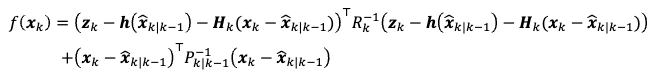
\[\mathbf{x}_k = f(\mathbf{x}_{k-1}, \mathbf{u}_{k}) + \mathbf{w}_k, \quad \mathbf{z}_k = h(\mathbf{x}_k) + \mathbf{v}_k\]

Idea: approximate it with linearization. For each update step, we can compute the Taylor expansion of the function, take the linear term, and then apply the Kalman filter.

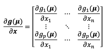
Linearization

The most straightforward method is to consider Taylor expansion:

\[\mathbf{g}(\mathbf{x}) = \mathbf{g}(\mathbf{\mu}) + \frac{\partial \mathbf{g}}{\partial \mathbf{x}}(\mathbf{\mu})(\mathbf{x} - \mathbf{\mu}) + \mathbf{O}(\|\mathbf{x} - \mathbf{\mu}\|^2)\]

where $\frac{\partial \mathbf{g}}{\partial \mathbf{x}}(\mathbf{\mu})$ is the Jacobian of the function at $\mathbf{\mu}$.

Therefore, given any non-linear function $\mathbf{x}k = f(\mathbf{x}{k-1}, \mathbf{u}_{k}) + \mathbf{w}_k$, we can:

1. compute the Jacobian to be the linear transformation matrix evaluated at the mean of the distribution:

   \[F_k = \frac{\partial f}{\partial x}(\hat{\mathbf{x}}_{k-1|k-1}, \mathbf{u}_k)\]

   so that the linearized model is, using Taylor expansion:

   \[\mathbf{x}_k = f(\hat{\mathbf{x}}_{k-1|k-1}, \mathbf{u}_k) + F_{k} \cdot (\mathbf{x}_{k-1} - \hat{\mathbf{x}}_{k-1|k-1}) + \mathbf{w}_k\]

   note that $f(\hat{\mathbf{x}}_{k-1\vert k-1})$ is a constant you can compute at each update step.

2. we can similarly apply linearization to the measurement model, with mean computed from the previous step $\hat{\mathbf{x}}_{k\vert k-1}$:

   \[H_k = \frac{\partial h}{\partial x}(\hat{\mathbf{x}}_{k|k-1})\]

   so that the linearized model is:

   \[\mathbf{z}_k = h(\hat{\mathbf{x}}_{k|k-1}) + H_k \cdot (\mathbf{x}_k - \hat{\mathbf{x}}_{k|k-1}) + \mathbf{v}_k\]

3. now all transformations are linear, we can reapply the Kalman filter to update the belief state, but the equations become a little different than before.

Extended Kalman Filter Derivations

Now, we derive the case of Kalman filters under which we use a linearized version of non-linear functions.

Extended Prediction Step

Now our motion model becomes:

\[\mathbf{x}_k = f(\hat{\mathbf{x}}_{k-1|k-1}, \mathbf{u}_k) + F_k \cdot (\mathbf{x}_{k-1} - \hat{\mathbf{x}}_{k-1|k-1}) + \mathbf{w}_k\]

and given the previous belief parameters $\hat{\mathbf{x}}{k-1\vert k-1}, P{k-1\vert k-1}$, we want to find out what’s the new mean and variance:

\[\mathbf{x}_k' \sim \mathcal{N}(\hat{\mathbf{x}}_{k|k-1}, P_{k|k-1})\]

It turns out that in this case, you will get:

\[\begin{cases} \hat{\mathbf{x}}_{k|k-1} = f(\hat{\mathbf{x}}_{k-1|k-1}, \mathbf{u}_k), & \text{new mean}\\ P_{k|k-1} = F_k P_{k-1|k-1} F_k^T + Q_k, & \text{new variance} \end{cases}\]

Therefore the new mean is just the non-linear function evaluated at the previous mean, and the new variance is the same equation but with the linearized approximation matrix $F_k$.

Extended Update Step

Now our measurement model becomes:

\[\mathbf{z}_k = h(\hat{\mathbf{x}}_{k|k-1}) + H_k \cdot (\mathbf{x}_k - \hat{\mathbf{x}}_{k|k-1}) + \mathbf{v}_k\]

then you can do the same thing to find what’s the new mean and covariance if you do the same procedure as before:

\[B(x_k) \propto p(\mathbf{z}_k|\mathbf{x}_k) B'(\mathbf{x}_k) = \exp(- \frac{1}{2} f(\mathbf{x}_k)) \propto \mathcal{N}(\hat{\mathbf{x}}_{k|k}, P_{k|k})\]

matching the terms that the final distribution is Gaussian, you will get: and you will find that:

Hence we get exactly the same as before

\[\begin{cases} \hat{\mathbf{x}}_{k|k} = \hat{\mathbf{x}}_{k|k-1} + K_{k} \tilde{\mathbf{y}}_k, & \text{new mean}\\ P_{k|k} = (I - K_k H_k) P_{k|k-1}, & \text{new variance} \end{cases}\]

except that:

• $\tilde{\mathbf{y}}k = \mathbf{z}_k - h(\hat{\mathbf{x}}{k\vert k-1})$ is the innovation using the non-linear function
• $K_k = P_{k\vert k-1} H_k^{T}S_k^{-1}$ is the Kalman gain using the linearized approximation
• $S_k = H_k P_{k\vert k-1} H_k^{T} + R_k$ is the innovation covariance using the linearized approximation

Summary of Extended Kalman Filter

In summary, given a prior belief state $\hat{\mathbf{x}}{k-1\vert k-1}, P{k-1\vert k-1}$, the update steps for the mean and covariances look like:

1. Prediction step with motion model:

   \[\begin{cases} \hat{\mathbf{x}}_{k|k-1} = f(\hat{\mathbf{x}}_{k-1|k-1}, \mathbf{u}_k), & \text{nonlinear}\\ P_{k|k-1} = F_k P_{k-1|k-1} F_k^T + Q_k, & \text{linear with Jacobian} \end{cases}\]

2. Update step with measurement model:

   \[\begin{cases} \hat{\mathbf{x}}_{k|k} = \hat{\mathbf{x}}_{k|k-1} + K_{k} \tilde{\mathbf{y}}_k, & \text{nonlinear}\\ P_{k|k} = (I - K_k H_k) P_{k|k-1}, & \text{linear with Jacobian} \end{cases}\]

   where you have:

   • $\tilde{\mathbf{y}}k = \mathbf{z}_k - h(\hat{\mathbf{x}}{k\vert k-1})$
   • $K_k = P_{k\vert k-1} H_k^{T}S_k^{-1}$
   • $S_k = H_k P_{k\vert k-1} H_k^{T} + R_k$

In practice:

• Just as efficient as regular KF, relatively robust in many real problems
• Less robust when uncertainty is high or models are locally very nonlinear

EKF Problem Cases

Key problem: linearization is evaluated at the mean of the distribution.

Intuitively, if your belief distribution is very narrow, then linearization near the mean would probably be fine:

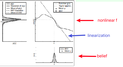
But if your belief distribution is spread out, then the linearization gives a lot of errors at the tails

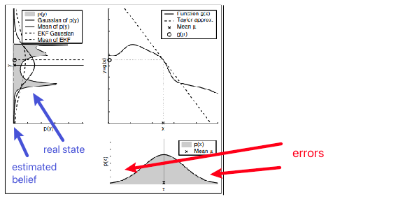
Alternatively, if your function is not very linear away from the point of linearization

EKF Localization

For example, consider a 1D robot where we had a good initial belief

Then let’s apply a motion model moving to the right, but with increased uncertainty

But then if you apply the measurement now:

and finally, if you moved again:

Motion Model Linearization Example

Now, let’s consider a planar mobile robot in SE(2):

Robot	Motion Model

where obviously the motion model is non-linear as it involves sin and cosine of the angle. So you can linearize it by taking the Jacobian:

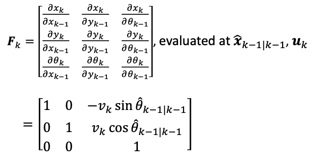
and then you can apply the EKF update steps as before.

Measurement Model Linearization Example

Now, le’s consider a measurement model being the range finder given a map:

Visual	Measurement Model

Again, it’s a non-linear function, so we need to linearize it by taking the Jacobian:

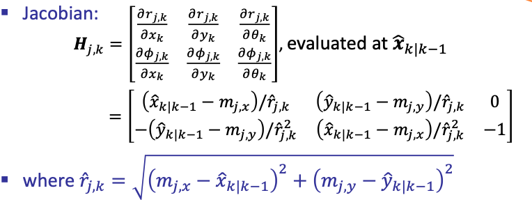
where we are looking at the $j$-th landmark at the $k$-th time step.

Problem: if there are $l$ land marks, the Jacobian will be very large and expensive to compute. Also the covariance matrix will $2l \times 2l$, and computing its inverse is expensive in EKF.

one common trick is to assume that the landmarks are independent, so that the updates for each landmark can be computed independently. With $l$ landmarks, we will get:

1. first initialize:

   \[\hat{\mathbf{x}}_{k|k} \gets \hat{\mathbf{x}}_{k|k-1}, \quad P_{k|k} \gets P_{k|k-1}\]

2. then for each landmark, compute independently:

   \[\begin{cases} \hat{\mathbf{x}}_{k|k} = \hat{\mathbf{x}}_{k|k} + K_{j,k} \tilde{\mathbf{y}}_{j,k}, & \text{new mean}\\ P_{k|k} = (I - K_{j,k} H_{j,k}) P_{k|k}, & \text{new variance} \end{cases}\]

   where:

   • $\tilde{\mathbf{y}}{j,k} = \mathbf{z}{j,k} - h_{j,k}(\hat{\mathbf{x}}_{k\vert k})$
   • $K_{j,k} = P_{k\vert k} H_{j,k}^{T}S_{j,k}^{-1}$
   • $S_{j,k} = H_{j,k} P_{k\vert k} H_{j,k}^{T} + R_{j,k}$

   and now $S^{-1}_{j,k}$ shown above is much easier to compute.

---

As an example, consider white circles as the landmarks, and the solid line being the actual movement. The dashed line is what the robot thinks it’s moving. The light gray is belief after motion model updates

And if you increase uncertainty in real measurement (e.g., sensor errors)

Data Association

Another practical problem is that, given $l$ measurements, we need to know which landmark it corresponds to in order to do the above computation. In practice, we need to estimate it since we don’t know the true correspondence.

Idea: use maximum likelihood. For each landmark given the current (mean) position, we can estimate the likelihood of an measurement being the landmark $l$ and then choose the one with the highest likelihood.

So then this will need to be implemented as a separate sub-rountine in the EKF algorithm:

1. given a measurement $\mathbf{z}_k$, compute the likelihood of each landmark $l$’s expected measurement:

   \[\mathcal{N}(h_j(\hat{\mathbf{x}}_{k|k}), S_{j,k})\]

2. associate $z_{i,k}$ with the landmark $j$ that maximizes the likelihood

and more tricks to clean this up include

• may first filter out landmarks that are very unlikely or similar to each other
• may add a mutual exclusion constraint to prevent a landmark from being associated with multiple measurements

Multi-Hypothesis Tracking

Previously we assumed that Kalman filters work with belief = unimodal Gaussian. This is quite restrictive, but

Idea: Instead of one Gaussian, our belief can be written as a mixture of Gaussians

Then what happens in KF? It can be still extended, with:

• apply KF to each of the Gaussian
• add a few correction terms (details omitted)

This could be useful for:

• initial robot belief is uncertain: it might be at 2 different places with high prob.
• In the extreme case, this can solve the data association problem by creating a mixture component for every possible feature-measurement correspondence!

in practice maintaining all the Gaussians is expensive, so a simple fix would be that we simply prune the components down to a fixed number after each filter update

Other Considerations for Kalman Filters

A few differenes:

• in Particle Filters obstacle regions are automatically avoided. EKFs cannot represent spatial constraints
• too many measurement features increase computation and possibility of mixing up features (e.g., the data association problem); too few may be insufficient for good estimation
• EKFs cannot incorporate negative information, e.g. absence of a feature: I don’t see a door X, therefore I cannot be at location Y.

Simultaneous Localization and Mapping

Previsouly we discussed localization methods assuming we know the map/obstacles in advance. In this section, we will:

• discuss how to perform mapping (by itself) assuming we know the robot’s state/measurements (localization)
• discuss how to perform localization and mapping simultaneously

So we can consider The posterior over all maps given data is Pr(𝒎

𝒙1:𝑘 , 𝒛1:𝑘 ) and independence

Occupancy Grid Mapping

A popular method to represent the map is to use an occupancy grid: the map becomes a grid world, and you want to know whether each cell is occupied by an obstacle or not.

Mathematically, we want to model:

\[\Pr(\mathbf{m} | \mathbf{x}_{1:k}, \mathbf{z}_{1:k})\]

where here we can assume that the history of robot states and measurements are given. $m$ would be like a vector of the size of the number of grids, modeling the probability of each cell being occupied.

Bayes Filter for Mapping

The above is difficult to even represent if you have a large map. Therefore, one assumption we can make is to assume each grid/cell’s occupancy is independent of others:

\[\Pr(\mathbf{m} | \mathbf{x}_{1:k}, \mathbf{z}_{1:k}) = \prod_{i} \Pr(m_i | \mathbf{x}_{1:k}, \mathbf{z}_{1:k})\]

so we can model the belief distribution of each grid cell independently. So how do we do not?

Recall that Bayes filter is a recursive way to update the belief state given the previous estimates:

\[\Pr( m_i | \mathbf{x}_{1:k}, \mathbf{z}_{1:k}) \gets \text{previous estimate } \Pr(m_i | \mathbf{x}_{1:k-1}, \mathbf{z}_{1:k-1})\]

Foolowing conditional independence between the latest observation $\mathbf{z}k$ and the history $\mathbf{x}{1:k-1},\mathbf{z}_{1:k-1}$ given the robot’s current state $\mathbf{x}_k$, we can write the above as:

\[\begin{align*} \Pr(m_i | \mathbf{x}_{1:k}, \mathbf{z}_{1:k}) &= \eta \Pr(\mathbf{z}_k | m_i, \mathbf{x}_{1:k}, \mathbf{z}_{1:k-1}) \Pr(m_i | \mathbf{x}_{1:k}, \mathbf{z}_{1:k-1}) \\ &= \eta \Pr(\mathbf{z}_k | m_i, \mathbf{x}_k) \Pr(m_i | \mathbf{x}_{1:k}, \mathbf{z}_{1:k-1})\\ &= \eta \frac{\Pr( m_{i} | \mathbf{x}_{k}, \mathbf{z}_{k}) \Pr(\mathbf{z}_k | \mathbf{x}_k )}{\Pr( m_i | \mathbf{x}_k)} \Pr(m_i | \mathbf{x}_{1:k}, \mathbf{z}_{1:k-1})\\ &= \eta \frac{\Pr( m_{i} | \mathbf{x}_{k}, \mathbf{z}_{k}) \Pr(\mathbf{z}_k | \mathbf{x}_k )}{\Pr( m_i )} \Pr(m_i | \mathbf{x}_{1:k}, \mathbf{z}_{1:k-1}) \end{align*}\]

where the second equality used conditional independence mentioned above, and the last equality used the independence of $m_i$ and $\mathbf{x}_k$ (dependent only if we have an observation $\mathbf{z}_k$).

Log Odds

However, the above is computationally not efficient because:

• computing the joint $\Pr(\mathbf{m} \vert \mathbf{x}{1:k}, \mathbf{z}{1:k})$ would end up multiplying a lot of probabilities
• there are three probabilities to compute for each cell $\Pr(m_i \vert \mathbf{x}{1:k}, \mathbf{z}{1:k})$

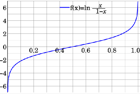
One trick to solve both issue would be using the log odds instead.

Consider the probability of observing an event $x$ as $\Pr(X)$, then define:

\[l(x) = \text{log odds} = \log \frac{\Pr(X)}{1 - \Pr(X)} = \log \frac{\Pr(X)}{\Pr(\bar{X})}\]

Visually, it would look like

This is useful because the log odd of $\Pr(m_i \vert \mathbf{x}{1:k}, \mathbf{z}{1:k})$ then becomes:

\[\begin{align*} l_{i,1:k} &= \log \frac{\Pr(m_i | \mathbf{x}_{1:k}, \mathbf{z}_{1:k})}{1 - \Pr(m_i | \mathbf{x}_{1:k}, \mathbf{z}_{1:k})}\\ &= \log \frac{\Pr(m_i | \mathbf{x}_{1:k-1}, \mathbf{z}_{1:k-1})}{1 - \Pr(m_i | \mathbf{x}_{1:k-1}, \mathbf{z}_{1:k-1})} \frac{\Pr( m_{i} | \mathbf{x}_{k}, \mathbf{z}_{k})}{ 1- \Pr( m_{i} | \mathbf{x}_{k}, \mathbf{z}_{k}) } \frac{ 1 - \Pr( m_i )}{\Pr( m_i )}\\ &\equiv l_{i,1:k-1} + l_{i,k} - l_{i} \end{align*}\]

so that:

• the term $\Pr(\mathbf{z}_k \vert \mathbf{x}_k )$ is cancelled as we compute the ratio
• adding log odds is numerically stable
• you have basically the “next log odd = previous log odd + log odd of $m_i$ given current measurement/states - log odd of prior”

The only challenge left is how do we model $l_{i,k}$?

Inverse Sensor Model

It turns out that $l_{i,k} = \log \frac{\Pr( m_{i} \vert \mathbf{x}{k}, \mathbf{z}{k})}{ 1- \Pr( m_{i} \vert \mathbf{x}{k}, \mathbf{z}{k}) }$ is also called a n inverse sensor model and there is no single best way to do this yet. The popular approach (next section) is do learn this from a machine learning model.

In some special case, however, there are methods that can estimate this. Consider we are using a beam sensor like this:

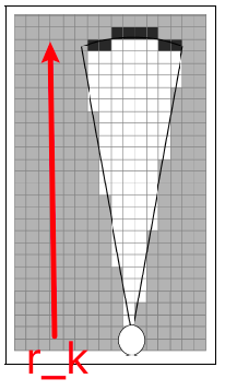
where $r_k$ is the distance from robot to the dark square. Then we can model this log odds by:

1. decrease log odds of cell closer than $r_k$ as they are likely free
2. increase log odds of cell physically around $r_k$ as they are likely occupied
3. no change for other cells

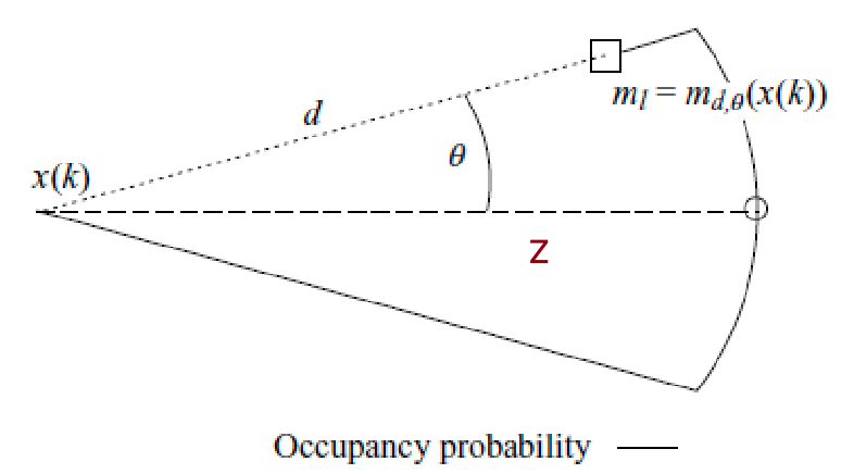
again, this is empirical, but works quite well. Implementation-wise, one can first consider a mixture of zero-mean gaussian over $\theta$ and a decreasing linear function of $r_k$ to capture uncertainty in both range and bearing

Then, given a measurement $z$ being the distance to the obstacle, we can update the distribution with a piecewise function on the left:

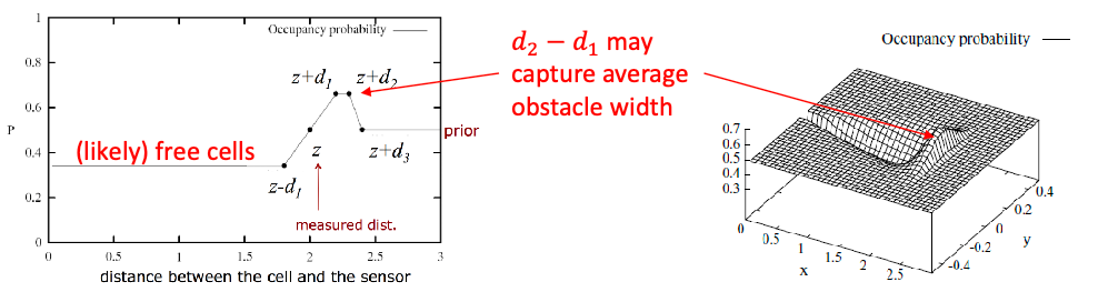
where $d_1, d_3$ are hyperparameters. A full mapping run using the above technique would look like:

Process	Mapped

Learning Inverse Sensor Models

But again, there is no closed-form solution to derive $\Pr( m_{i} \vert \mathbf{x}{k}, \mathbf{z}{k})$, an inverse model, given the forward model $\Pr( \mathbf{z}{k} \vert \mathbf{x}{k}, m_{i} )$ using Bayes.

So other pratical yet pretty good trick is to learn a model using supervised learning:

1. generate training data ${(\mathbf{x}_k, \mathbf{z}_k, m_i)}$ by sampling from known maps, robot states, and measurements
2. train a model to predict $m_i$ given $\mathbf{x}_k, \mathbf{z}_k$ using a neural network or other machine learning models

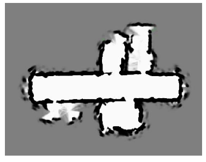
Independence Assumption

Finally, another problem of our current method is that we are assuming the occupancy of each cell is independent of each other. This is may not be true in practice:

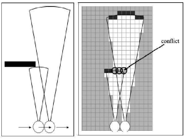
where in the above example, certain cells (e.g., the conflict shown above) depends on knowing its immediate neighbor being an obstacle.

In practice, this can be somewhat alleviated by:

• narrower beam sensors like lidar can help alleviate this issue
• or somehow learn this as well from machine learning models (above)

SLAM

Finally, here we discuss how to do localization and mapping simultaneously. The idea is to include the map as part of the state vector, and make corresponding modifications to the EKF or Particle Filter algorithm.

EKF-SLAM

Suppose we know that our map consists of $N$ landmarks, but we are not sure where they are ($N$ can increase as the algorithm goes).

Then we can model state $\mathbf{x}$ = robot state + landmark location. This means that we consider:

\[\mathbf{x} = (x,y,\theta, m_{1x},m_{1y}, ...,m_{Nx},m_{Ny}) \in \R^{3+2N}\]

for a robot in 2D space, and then apply the EKF algorithm as before (with some modifications below)

First, we note that our covariance matrix becomes $P \in \R^{(3+2N)\times (3+2N)}$

\[P = \begin{bmatrix} P_{xx} & P_{xm}\\ P_{mx} & P_{mm} \end{bmatrix}\]

where $P_{xx} \in \R^{3\times 3}$ is the covariance of the robot state, $P_{mm} \in \R^{2N\times 2N}$ is the covariance of the landmarks, and $P_{xm} \in \R^{3\times 2N}$ is the cross-covariance between the robot state and the landmarks.

Algorithmically:

1. we can initialize with 1) robot initial position and landmark being uncorrelated, and 2) infinite variance for the landmarks since we have no idea where they are:

   \[P_{xx,0} = \mathbf{0}^{3\times 3}, \quad P_{mm,0} = \infty \times \mathbf{I}^{2N\times 2N}, \quad P_{xm,0} = \mathbf{0}^{3\times 2N}\]

   and some robot state guess $\mathbf{x}0$ and landmark guess $\mathbf{m}{0}$.

   Note that we can also add landmarks as we go (e.g., if our data association model found some landmark estimate to be extremely low = likely a new landmark, or there is a signature we can use to check if its a existing landmark). In this case, we can add terms to the covariance/mean with a non-zero initialization:

   \[\begin{bmatrix} \hat{m}_{jx} \\ \hat{m}_{jy} \end{bmatrix} = \begin{bmatrix} \hat{x} \\ \hat{y} \end{bmatrix} + \begin{bmatrix} r_j \cos(\hat{\theta} + \phi_j) \\ r_j \sin(\hat{\theta} + \phi_j) \end{bmatrix}\]

2. predict step given some movement/motion model (e.g., a vecolity model)

   

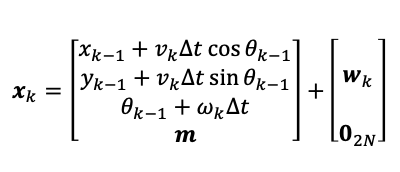
   where we do not update the landmarks position since they don’t move. We can then linearize this and show that

   

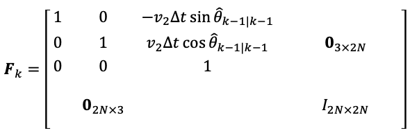
   then we apply the same prediction step to both the covariance and the mean. Note that given the nature of obstacles not moving, $P_{mm}$ will remain unchanged while $P_{xx}$ and $P_{xm}$ will change in this step.

3. update step then you can compute your observation $z$​ but with landmark location (you estimated) from previous step

   

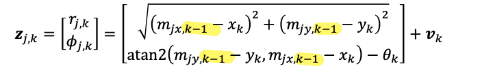
   and again, we need to linearize the above ($h(\cdot)$) using the Jacobian $H_{i,j}$ evaluted at the estimated state/landmark location:

   

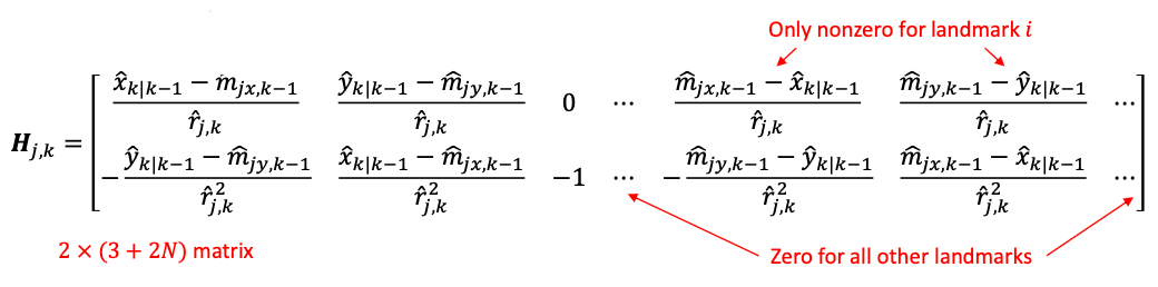
   This would give a $2 \times (3+2N)$ matrix $H_k$. Since landmarks do not affect each other, we will only have two additional non-zero columns for each landmark $j$. With this, we can apply the same measurement step from EKF to both covariance and mean updates.

In summary, EKF-SLAM equations are near identical to the regular EKF algorithm:

1. predict step considers:

   \[\begin{cases} \hat{\mathbf{x}}_{k|k-1} = f(\hat{\mathbf{x}}_{k-1|k-1}, \mathbf{u}_k), & \text{nonlinear}\\ P_{k|k-1} = F_k P_{k-1|k-1} F_k^T + Q_k, & \text{linear with Jacobian} \end{cases}\]

   Note that given the nature of obstacles not moving, $P_{mm}$ will remain unchanged while $P_{xx}$ and $P_{xm}$ will change in this step.

2. update step considers:

   \[\begin{cases} \hat{\mathbf{x}}_{k|k} = \hat{\mathbf{x}}_{k|k-1} + K_{k} \tilde{\mathbf{y}}_k, & \text{nonlinear}\\ P_{k|k} = (I - K_k H_k) P_{k|k-1}, & \text{linear with Jacobian} \end{cases}\]

   where you have:

   • $\tilde{\mathbf{y}}k = \mathbf{z}_k - h(\hat{\mathbf{x}}{k\vert k-1}, \hat{m}_{k-1})$ depends on your estimate of the landmark
   • $K_k = P_{k\vert k-1} H_k^{T}S_k^{-1}$
   • $S_k = H_k P_{k\vert k-1} H_k^{T} + R_k$

note that although $H_k$ is sparse, the Kalman gain $K_k \in \R^{3 \times (3+2N)}$ is generally dense. This is because it incorporates correlations/updates between landmarks that were previously seen.

For example, if we have two landmarks, then $F_k \in \R^{(3 + 2\times 2)\times (3 + 2\times 2)}$ matrix

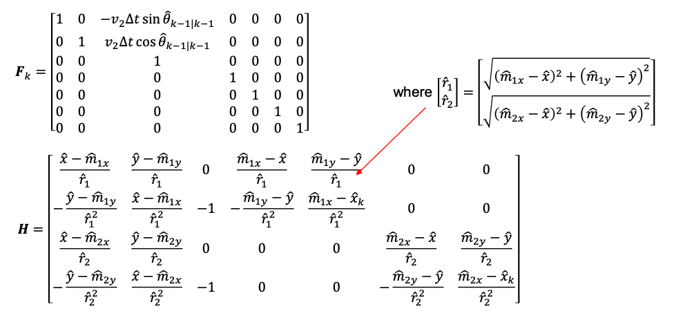
where we dropped the $k$ subscript in $H=[H_1, H_2]^{T}$ for each landmark to save space. Notice that the last four columns in $H$ is block diagonal: this is because the $x,y$​​ for a landmark is independent of the other landmarks.

Note in this section it seems that mapping is not very hard: this is because we have simplified the map to simply be the location of obstacles. In practice, if you need Occupany Grid, then you really need Occupancy Grid Mapping.

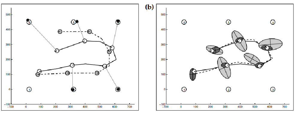
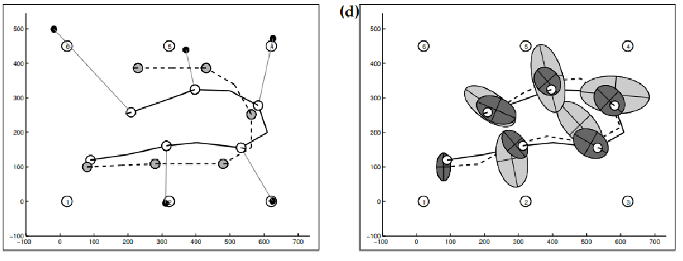
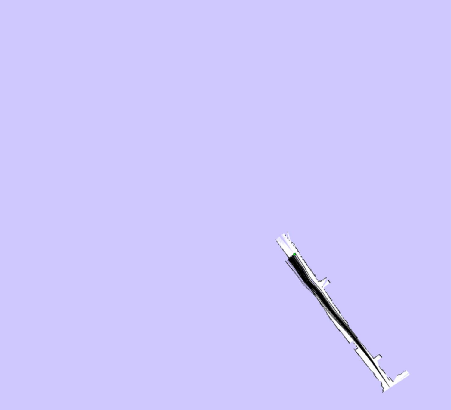
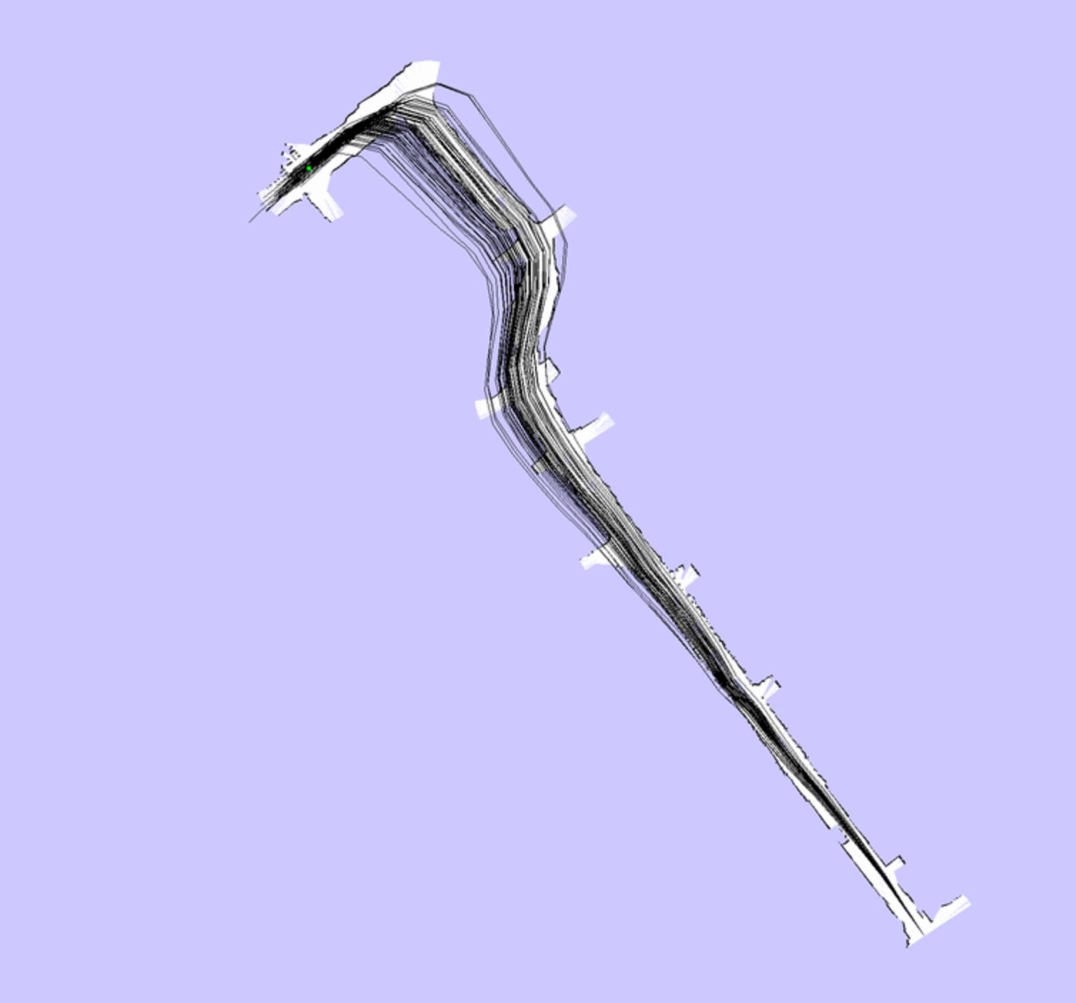
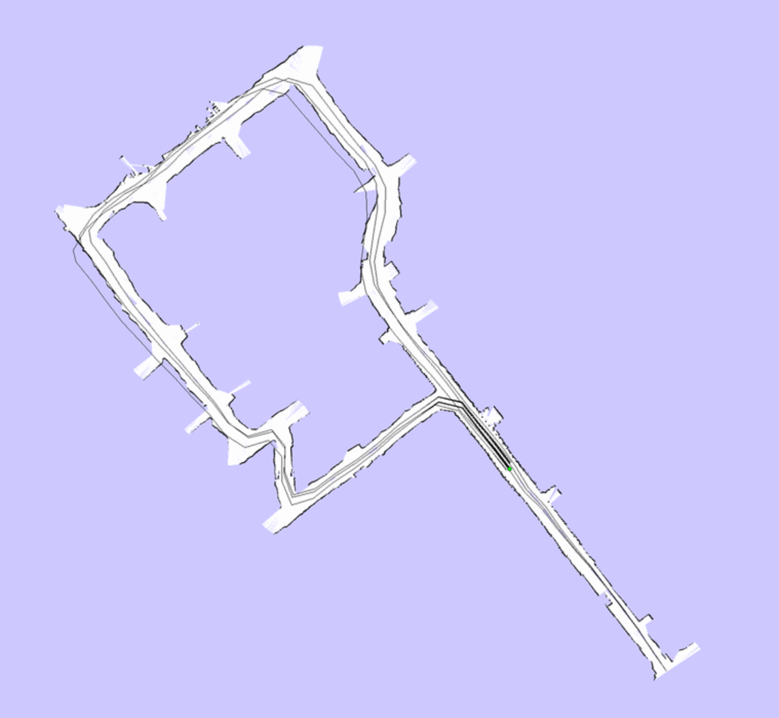
EKF-SLAM Example

Visually, let the red small dots be the actual landmarks, and gray dots be the actual robot’s path. Then our estimate of mean and variance may look like:

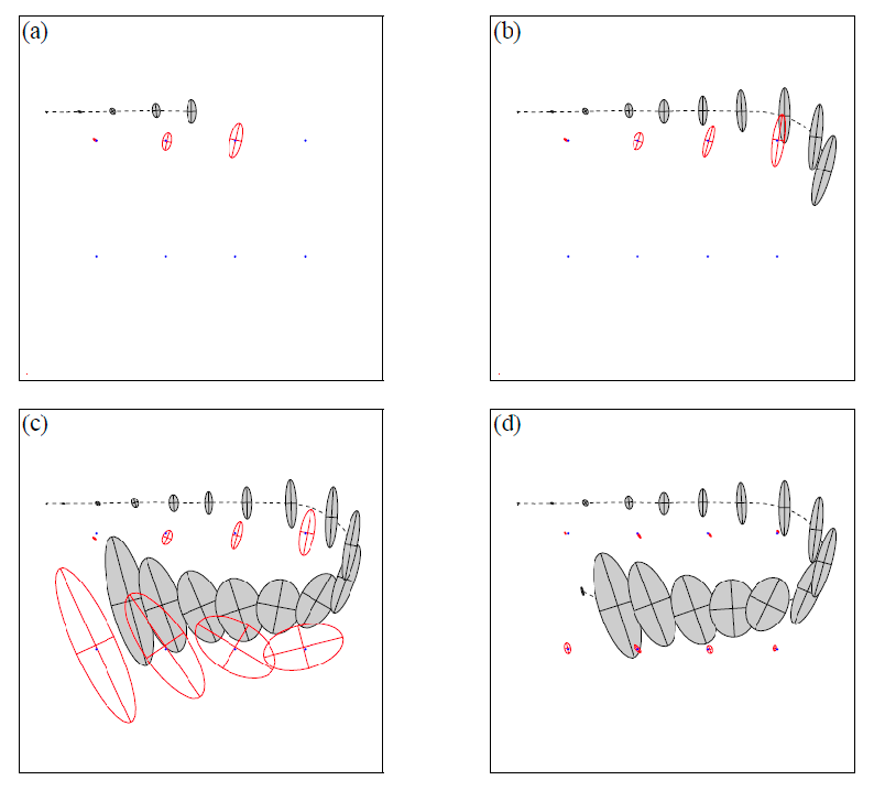
note that:

• in the beginning, as the robot moves and sees new landmarks, its own uncertainty grows. Landmark uncertainties also grow since they depend on robot uncertainty
• but uncerintaty of landmarks are correlated: once we have a low uncertainty for a landmark (in (d) as we saw the top left landmark again), the uncertainty of the other ones decrease as it indicates our estimate of landmarks were likely all correct.
• With sufficient observations, the individual variances (uncertainties) of both robot state and landmarks converge toward a lower bound = becomes certain of its position and the landmarks

Problems with EKF-SLAM:

• Complexity of each EKF iteration is quadratic in the number of landmarks = cannot handle very large maps
• Cannot take advantage of sparsity, as all landmarks eventually become fully correlated
• Still subject to the usual limitations of EKFs (nonlinearity, high uncertainty)
• data association problem becomes more critical in this case

Particle Filters for SLAM

Recall that in Particle Filters, we had each particle representing a clone of the robot. Consider a simple idea similar to EKF SLAM, where now each particle represent the robot + a map configuration.

The problem with naively doing the above is its cloning the map too much.

• in EKF, we have one distribution over the robot state
• in particle filter, each particle itself is certain of its robot state, but the distribution is recovered by the distribution of the particles.

Therefore, the key idea is to assume each particle has no uncertainties about its state, and hence the partcle can itself solve its own mapping problem.

Rao-Blackwellization

The key idea is implemented with factoring the state distribution $\mathbf{x}=[\mathbf{x}_{1:k}, \mathbf{m}]$ into two parts:

\[\begin{align*} \Pr(\mathbf{x}_{1:k}, \mathbf{m} | \mathbf{z}_{1:k}, \mathbf{u}_{1:k}) &= \Pr(\mathbf{x}_{1:k} | \mathbf{z}_{1:k}, \mathbf{u}_{1:k}) \Pr(\mathbf{m} | \mathbf{x}_{1:k}, \mathbf{z}_{1:k}, \mathbf{u}_{1:k})\\ &= \Pr(\mathbf{x}_{1:k} | \mathbf{z}_{1:k}, \mathbf{u}_{1:k}) \Pr(\mathbf{m} | \mathbf{x}_{1:k}, \mathbf{z}_{1:k})\\ &= \Pr(\mathbf{x}_{1:k} | \mathbf{z}_{1:k}, \mathbf{u}_{1:k}) \prod_{i} \Pr(m_i | \mathbf{x}_{1:k}, \mathbf{z}_{1:k}) \end{align*}\]

where the last equality is because the map is independent of the control sequence $\mathbf{u}_{1:k}$​​. Then

• the term $\Pr(\mathbf{x}{1:k} \vert \mathbf{z}{1:k}, \mathbf{u}_{1:k})$ can be represented purely by the density distribution of our partciles
• the term $\Pr(m_i \vert \mathbf{x}{1:k}, \mathbf{z}{1:k})$ is simply the individual landmark estimate given a robot state/measurement.

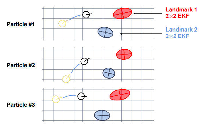
FastSLAM

Using the above factorization, we can do

FastSLAM: Use normal particle filter for the robot state, and then for each particle, use EKF to model each of the landmarks.

This means that given $M$ particles, we will consider tracking:

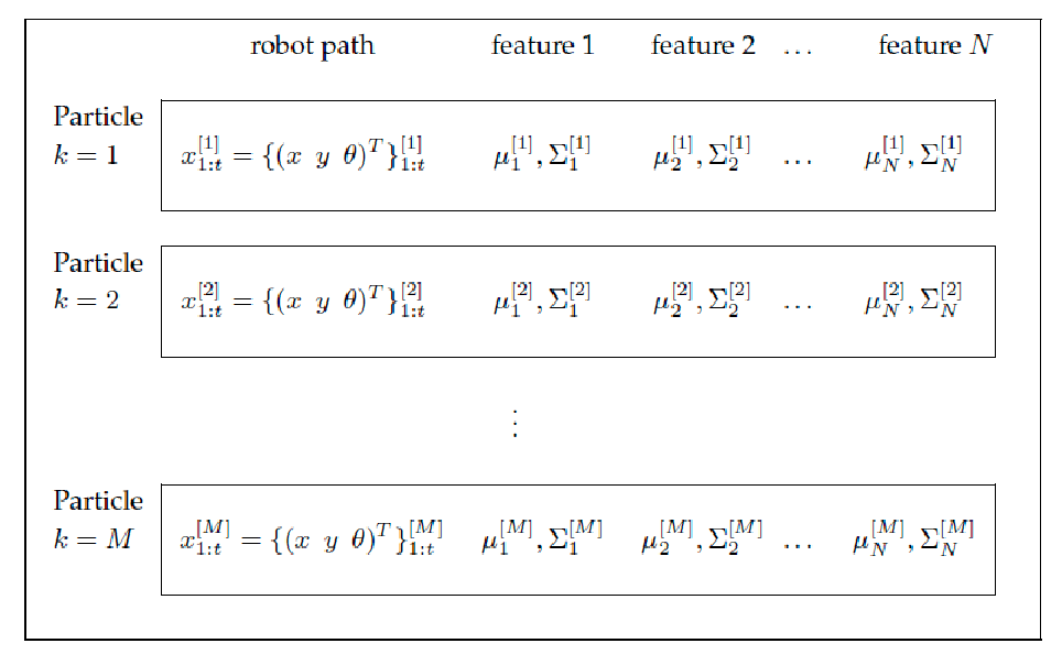
where:

• for each particle, we track its trajectory and its own estimate of landmark’s mean and variance:
• each landmark’s mean and covariance is also modelled independently in this algorithm: much easier to compute as its simply $\R^{2 \times 2}$ for each landmark!
• this results in 1 filter (normal particle filter) of the robot’s state (the above), and $MN$ filters for landmarks (one EKF filter for each particle and each landmark).

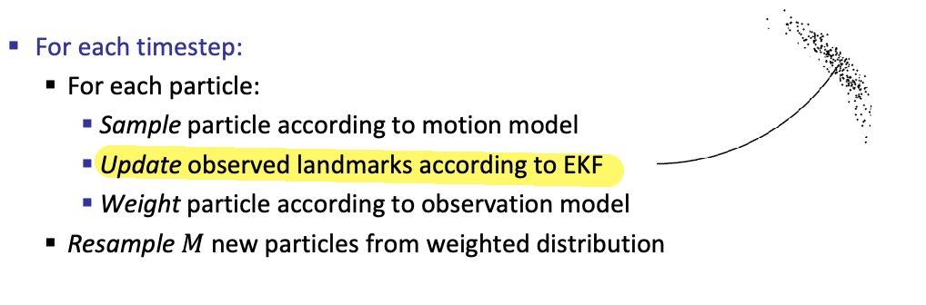
Overall, the algorithm is similar to the normal particle filter:>

In summary, FastSLAM equations are near identical to the regular particle filter algorithm:

The only difference is that we will be using EKF to model the landmarks, and the re-weighing operation will depend on our estimate of the landmarks.

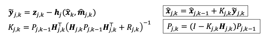
FastSLAM: updating landmarks

For each landmark, consider a Gaussian distribution for each landmarks’ position. Then we can model this using mean and covariance matrices. Specifically, we can show that for landmark $j$ with a measurement $z_{j,k}$, we can update our estimate with:

\[\Pr(m_{j,k} | \mathbf{x}_{1:k}, \mathbf{z}_{1:k}) \propto \Pr(\mathbf{z}_{j,k} | m_{j,k}, \mathbf{x}_{k}) \Pr(m_{j,k} | \mathbf{x}_{1:k-1}, \mathbf{z}_{1:k-1})\]

which can then be derived using EKK update steps! THis means we can do linearized models and update the mean and covariance with for each landmark $j$ with:

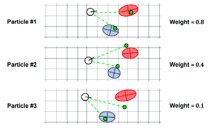
FastSLAM: Weighing

Finally, we want to re-weight each particle with the likelihood of seeing the measurement $z_k$ given the particle’s estimate of the map and its current position:

\[w = \Pr(\mathbf{z}_k | \mathbf{x}_k, \mathbf{m}_k) = \prod_{j} \Pr(\mathbf{z}_{j,k} | m_{j,k}, \mathbf{x}_k)\]

Then each of the weight can be obtained by modeling a Gaussian

\[w_{j} = \frac{1}{\sqrt{(2\pi)^2 |S_{j,k}|}} \exp\left(-\frac{1}{2} (\mathbf{z}_{j,k} - h_{j,k}(\mathbf{x}_k, m_{j,k}))^T S_{j,k}^{-1} (\mathbf{z}_{j,k} - h_{j,k}(\mathbf{x}_k, m_{j,k}))\right)\]

where $S_{j,k} = H_{j,k} P_{j\vert k-1} H_{j,k}^{T} + R_{j,k}$.

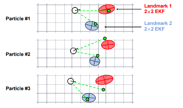
FastSLAM: Example

Consider the case of using $N=3$ particles, and there are 2 landmarks. Initially:

Let the green dots be the actual measurement made, and each particle can compute independently covariance updates of landmarks

finally, reweight and resample

An example in real life:

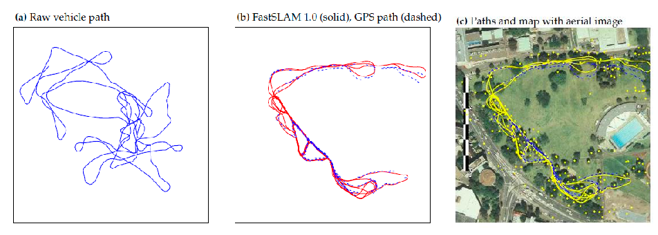
With an animated example:

Beginning	More Obstacles Seen	Loop Closure

Comparing SLAM Algorithms

In practice you need to do data associations yourselves.

• With EKF-SLAM, we can only compute a single association per measurement
• With FastSLAM, each particle can compute its “best” correspondence for the same measurement, e.g. using maximum likelihood (actually an advantage)

With map updates:

• With EKF-SLAM, you update a single map update
• With FastSLAM, each particles can maintain their own maps by adding or removing landmarks when necessary

For both SLAM, convergence occur when loop is closed

• particle filters face the problem of particle deprivation: before loop is closed, you need to maintain particle diversity otherwise estimate could converge to a wrong estimate = bias

  

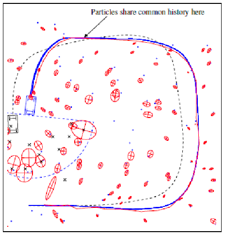
• resampling particles = as particles are resampled, we lose most of the estimated histories

  • in an extreme case, particle filters might not even be able to close the loop: suppose you just observed obstacle $m_j$ but also lost all particles that saw it before
  • this is less of a problem for EKF-SLAM, since all historical correlations are tracked

Some fixes for FastSLAM:

• simply have more or insert random particles to alleviate deprivation
• In FastSLAM 2.0, they use a proposal distribution that takes into account both motion and measurements

Robot Perception and Vision

Implementation-wise, previous sections were considering algorithms that runs on “already processed data”, i.e., observations as simple numbers/vectors. However, in practice, robots need to perceive the world using sensors, and interpret the data to make decisions.

Modern robots have access to a wide variety of different sensors:

• Proprioceptive sensors measure internal state, e.g. motor speed, joint angles
• Exteroceptive sensors acquire external environment information, e.g. distance measurements, light intensity

Examples include

In later subsections, we will instead focus on vision sensors/models that takes in camera input and returns measurements. This means:

Vision-type sensors have two key ingredients:

• Digital cameras (e.g., color, depth, stereo) are sensors that capture light and transform them to digital images
• Computer vision is concerned with acquiring, processing, and understanding those digital images in order to extract symbolic information

This means that we will be tranforming our “mapping” or “pose estimation” tasks to become:

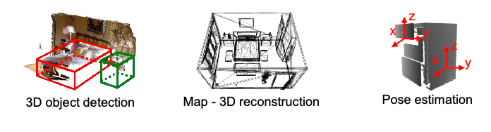
Image Representation and Filtering

This section assumes you are familiar with basic CV approaches.

• images are most often represented as a grid of pixel values $I(x,y)$

  • brightness adjustment $I(x,y)+\beta$
  • contrast adjustment: $\alpha I(x,y)$

• another way to processes those images is filtering

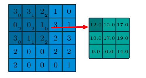
  • Spatial filters transform images using functions on pixel neighborhoods (i.e. convolution)

    \[I'(x,y) = F*I = \sum_{i=-M}^{M}\sum_{j=-N}^N F(i,j)I(x+i, y+j)\]

    where $F$ is a kernel with shape $(2M+1)\times (2N+1)$. Usually this kernel is a square:

    

  • examples of simple filters include:

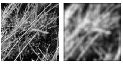
    • moving average filter:

      \[B = \frac{1}{9}\begin{bmatrix} 1 & 1 & 1\\ 1 & 1 & 1\\ 1 & 1 & 1 \end{bmatrix}\]

      this will basically blur an image

      

    • sharpening filter:

      \[S = \begin{bmatrix} 0 & 0 & 0\\ 0 & 2 & 0\\ 0 & 0 & 0 \end{bmatrix}\]

      this will sharpen the image

      

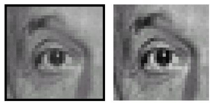
    • Gaussian filters; also achieves blurring, but weights are defined proportional to a Gaussian centered at each pixel

      

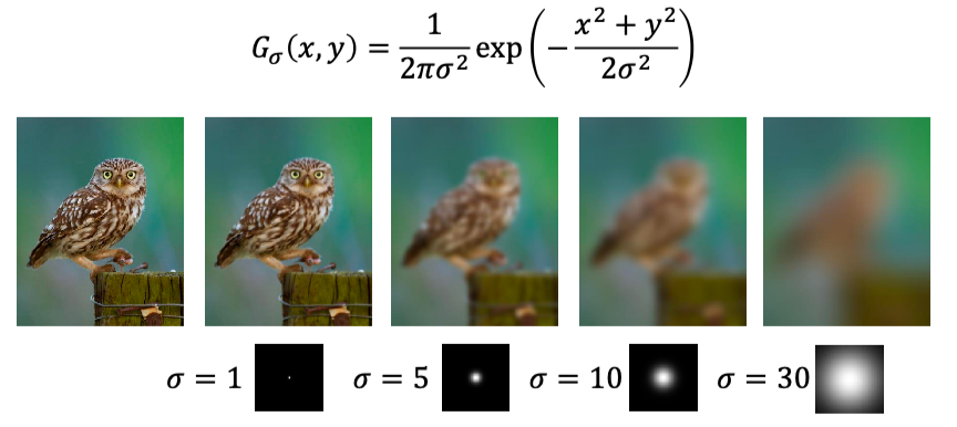
But recall that the goal is to understand what is in the image. This then includes:

• edge detection: when intensities are changing in a certain direction, it is “and edge”.

  Sobel detector	Result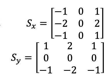

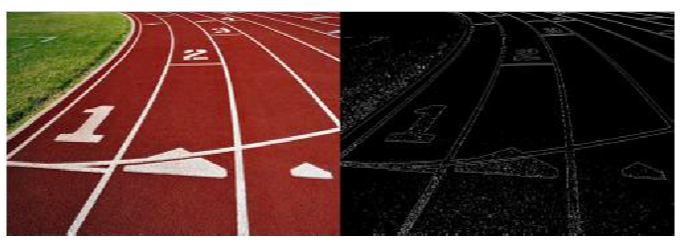
  There is also Canny detector is a multi-stage algorithm involving Gaussian smoothing and thresholding

  

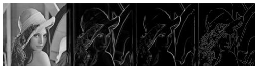
• corner detection: a point with large changes in intensity in all directions. In general, corners can be more directly used for 3D reconstruction and panorama stitching

  

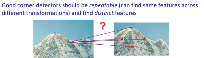
  More generally, image descriptors are features that can be compared across images, useful for object detection and matching

  

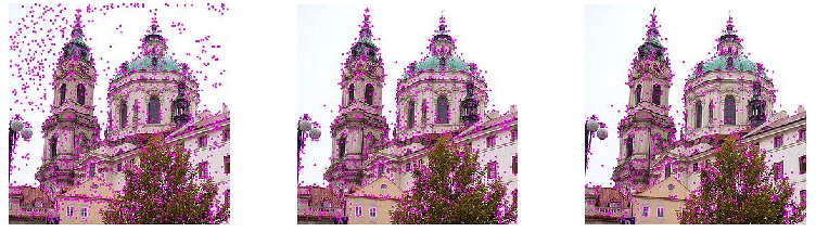
  there are many existing detection algorithms to do the above, e.g., SIFT (scale-invariant feature transform)

Point-Cloud Registration

Suppose we have two point clouds, and we want to want to find a spatial transformation that aligns them. This task can be useful for:

• finding globally consistent model
• 3D reconstruction and pose estimation
• data association in SLAM (see ICP later)

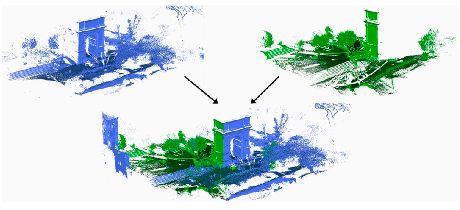
Since it is to figure out a transformation, this can be formulated mathematically as minimizing an error between one set of points and a transformation of the other set

And it turns out that if this transformation is a rotation followed by a translation, then there is a closed-form solution.

1. given two set of points $X= {x_1, …, x_n}$ and $P={p_1, …, p_n}$ and suppose they are associated already $(x_i, p_i)$

2. we can consider a transformation such that the following is minimized:

   \[E(R, \mathbf{t}) = \sum_{i=1}^{n} || \mathbf{x}_i - (R\mathbf{p}_i + \mathbf{t}) ||^2\]

3. then there is a closed formed solution:

   1. first re-center the data by:

      \[X' = X - \mu_x, \quad P' = P - \mu_p\]

   2. then compute a outer product matrix:

      \[W = \sum_{i=1}^{n} \mathbf{x}_i \mathbf{p}_i^T\]

      and perform SVD on $W = U \Sigma V^T$.

   3. then the optimal solution is given by:

      \[R^* = UV^T, \quad \mathbf{t}^* = \mu_x - R^* \mu_p\]

      which would minimize the error $E(R, \mathbf{t})$.

But then how do we find the data association with this?

ICP

One simple algorithm is just iteratively: estimate an association, compute the best solution and its error, provide a better estimate, and repeat.

And this leads us to ICP:

Iterative closest point (ICP): Iterate between estimating the correspondences by finding closest points and solving the least squares problem

but of course, this method:

• can be computationally intensive, especially with correspondence estimation
• Convergence depends on the initial guess and presence of noise and outliers
• Will generally converge to a local optimum, no guarantee of global optimal

ICP Improvements

Several lines of improvements on its efficiency and robustness:

• use $k$-d tree to increase the efficiency of finding closes points
• apply variable weighting to different pairs of points, e.g. lower weights to pairs that are very far apart or deemed less informative
• detecting outliers and ignore them in computations (see next section)

Random Sample Consensus

In general, detecting outlier data and removing them from your method is useful both in ICP and other CV problems. One common method is RANSAC:

RANSAC: Iterative algorithm for parameter estimation and outlier detection

The general approach is to:

1. randomly subsample from the full dataset
2. fit a model (e.g., a line shown in green below)
3. test all the data using the model to determine a consensus set (data that is consistent with this line) under some threshold
4. repeat, and keep the model that has the largest consensus set.

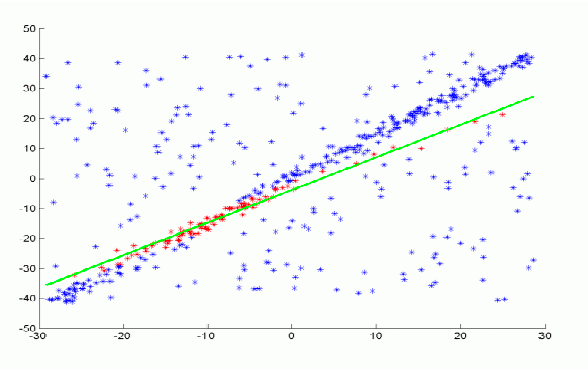
Since each of this loop is independent, one can compute this in parallel.

Convolutional Neural Networks

This section assumes you are familiar with basic CV approaches. So we will skip through the basics, and only keep some relevant information here.

Since images are large in dimension, CNN based approaches are very parameter efficient:

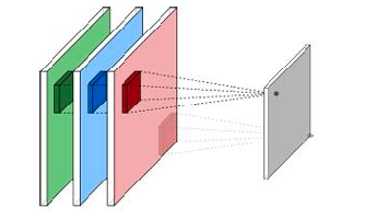
The set of outputs from all filters make up a new image called an activation map. This means you can:

1. each CNN can apply more than 1 kernel. Since the above applied one kernel and obtained an output of $(1, W,H)$ matrix, using $N$ kernels in a layer gives you back matrices of $(N, W, H)$.

2. then you can just stack those CNN layers, and learned features typically progress from more primitive (edges/corners) to more high-level

   

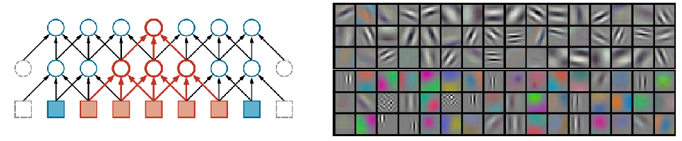
   to achieve this, typically the the receptive field (i.e., size of kernel) of a filter also increases with each layer

And other common layers used in CNN today include:

• Pooling layers: downsample and shrink the image. This can also be useful to prevent overfitting. This can implemented similarly to filters

  

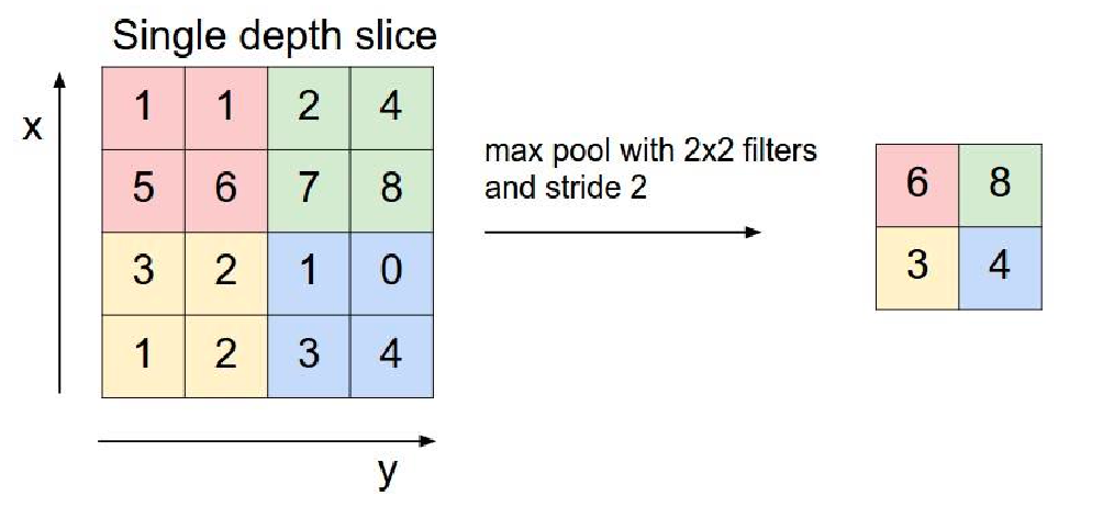
• Nonlinear activations: since convolution is still a linear operation, we still need nonlinear activation functions (e.g., RELU, GeLU, etc) to achieve better performance

Finally, the actual “classification task” is done by a few layers of FFNN:

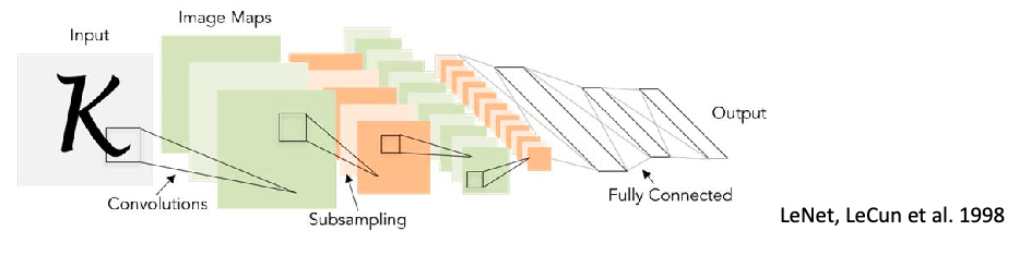
So in this view, CNN are mostly used to perform feature extraction efficiently, and the last regular FFNN layers + softmax performs the actual classification.

Reinforcement Learning

With both increasing computational power and complexity of robots, it is often desirable to learn models from data rather than derive them analytically. The idea is therefore to do RL from data.

But of course, data cannot solve everything:

• Curse of dimensionality—robots can be very high-dimensional systems
• We often only see data from a small part of the C- or state space
  • Probabilistic learning methods can help robot to infer missing information
• Real robots may also need to also consider effects such as friction
• To ensure sufficient richness in your data, may need lots of exploration, artificial noise while collecting data

Additionally, learning algorithms may also need to consider, given the data:

• there is often massive amounts of data coming through sensors -> need to discern what is useful
• need fast, real-time planning/execution algorithms
• May want to incorporate prior knowledge, active learning by interacting with humans for data labeling
• real life are non-stationary systems: Time-dependent dynamics, changing environments

RL Basics

We will go through RL quickly, assuming you are already familiar with most RL concepts. The key difference between SFT and RL is that the latter is learning through interaction/experience, whereas the former is fully offline.

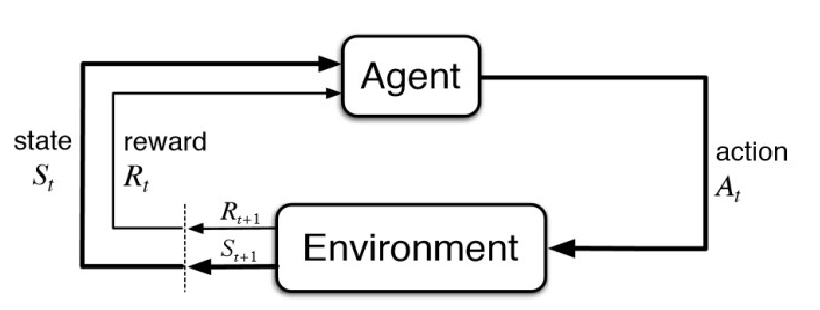
Example RL tasks in robotics look like:

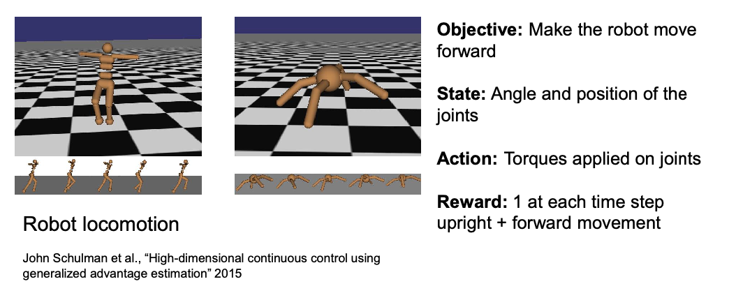
Example: Grid World

Consider the following setup

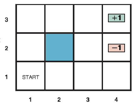
where:

• States and actions: Agent can choose to move in one of four cardinal directions from a given state, except at terminal states

• Transition function (motion model) $\Pr[s’\vert s,a]$: Probability distribution of successor states, given starting state and action. For example, it may be non-deterministic:

  

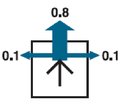
• Reward function: $\pm1$ for terminal states; constant living reward (e.g., $0$) for all other transitions

And then you can define value functions and action value functions as:

\[V^\pi(s) = \mathbb{E}_{\pi}\left[\sum_{t=0} \gamma^t r_t | s_0=s \right], \quad Q^\pi(s,a) = \mathbb{E}_{\pi}\left[\sum_{t=0} \gamma^t r_t | s_0=s, a_0=a \right]\]

where $\gamma\in(0,1]$ can be used to: 1) avoid infinite value functions if all rewards are positive, and 2) models how human may not lookahead to much.

In the case of a grid world, we can directly find the optimal value function $V^,Q^$, and hence extract the optimal policy $\pi^*$​. The idea is to use Bellman’s optimality equation and iteratively run:

\[Q(s,a) \gets \mathbb{E}_{s'}[R(s,a) + \gamma \max_{a'}Q(s',a')]\]

visually, applying the equation above will change the values near the terminal states with non-zero reward first, and then slowly propagate to all the remaining states. Finally, after this converged to $Q^$, we can extract $\pi^ = \arg\max_a Q^*(s,a)$​.

For DL methods, this will become:

1. sampling $(s,a,r)$​ observations
2. update the $Q$ network using the equation above
3. balance exploration-exploitation to select next action to do (typically $\epsilon$-greedy)
   • want to balance exploration with exploitation to avoid pure random walks

Deep Q-Network

The idea is to use ConvNet + RL to play games like Atari. This can be done by modeling the ConvNet as $Q_\theta$ and:

1. consider a loss function as:

   \[L_i(\theta_i) = \mathbb{E}[ (y_i - Q_{\theta_i}(s_t, a_t))^2]\]

   for your network at the $i$-th iteration. Since there is no label/ground truth $Q^*$, you can use

   \[y_i = \mathbb{E}_{s'}[r + \gamma \max_a Q_{\theta_{i-1}}(s_{t+1},a)]\]

   note that this is also an unbiased estimator of the optimal $Q^*$, if the above $Q_\theta$ has loss converges to zero.

2. play the game while training your model with the loss above.

The general policy-iteration paradigm for DL therefore looks like:

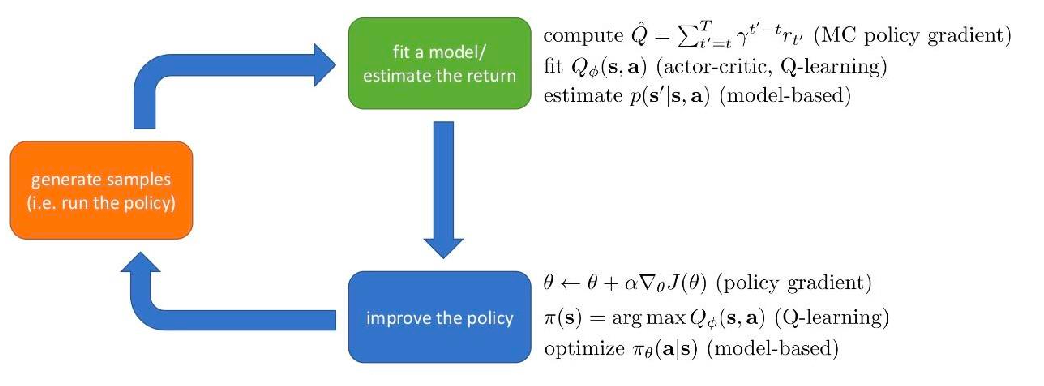
Imitation Learning

Many specialized tasks (especially those pertaining to humans) are difficult to define, program, and generalize from scratch. The idea is then to start with imitation learning, before considering RL.

On this approach. there can be many different ways of obtaining demonstration data

• Kinesthetic teaching: Physical guidance of the robot.

  • i.e., actually forcing the robot (e.g., arms) to do stuff

    

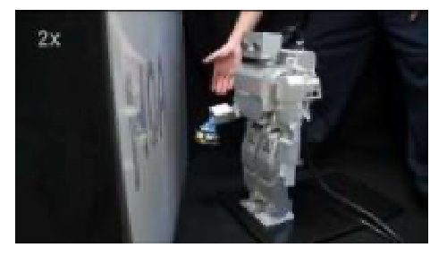
  • No explicit physical correspondence is needed

• Teleoperation: User has same perception as the robot.

  

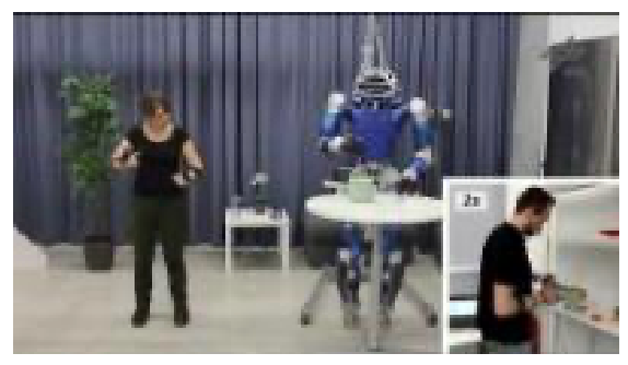
  • Can train robots from a distance or remotely
  • Difficult to perform low-level motion demonstrations

• Imitation: Directly recording human motions

  • Use of motion tracking systems, e.g. vision or wearable motion sensors
  • Need to solve human-robot correspondences

With these data (typically ~hundreds of demonstrations)

Typically we learn either policies, rewards/costs, or plans from these demonstrations.

• note that if we try to learn underlying models or reward functions instead, this goes into the framework of inverse reinforcement learning. One motivation for this is that for some tasks, the reward ($R^$) is often more succinct and robust than optimal policy ($\pi^$)
• if learning complex tasks, we try to break down them down into a sequence of sub-tasks or primitive actions—a plan
• Training a mapping going directly from raw pixels or observations to commands or actions is also known as end-to-end learning

For example

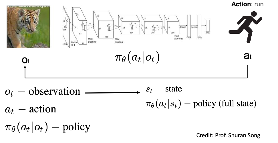
Challenges of Real World RL

Practical challenges:

• Discretization of continuous state and action spaces dramatically increases their dimensionality
• Real-world samples can be unreliable, expensive, and slow
• Robots must explore safely.
• Small modeling errors can lead to large error accumulations in unstable tasks
• Simulation bias—well-trained sim models may translate poorly to real systems