COMS6998 Spoken Language Processing

Logistics and Introduction

Syllabus:

• Mainly its weekly reading + posts
• 5% class participation (attendance at EoClass), 20% weekly post, and 75% from three HWs
• See for details cs.columbia.edu/~julia/courses/CS6998-24/syllabus24.html
• TA office hours:
  • Ziwei (Sara): CESPR714 M3-4pm
  • Debasmirta: CESPR 714 TH2-4pm
  • Yu-Wen Chen: Zoom FR 2-4pm
• a very useful reference I found: Introduction to Speech Processing — Introduction to Speech Processing (aalto.fi)
• a very useful Praat scripting reference: Sound (uva.nl)

Introduction

• Spoken language processing = not only what you say, but also how you say it.

• intonation contour: notice the difference between

  • You’re going. (statement)
  • You’re going? (question)

  and the fact that you can convey the two meaning without explicitly saying it ends with . or ?

• by just listening to how a person is saying things, you can learn about his/hers personality, mental health, etc.

• current and past challenges in spoken language processing:

  • e.g., “Do you live at 288 110th street?” is different from just pronouncing the numbers as-is
  • e.g., “They city hall parking lot was chock full of cars.” notice where pause are inserted between phrases.

From Sounds to Language

Linguistic sounds: how are sounds produced, and what sounds are shared by languages X and Y?

Motivation:

• sometimes sounds you produce can affect your thinking. e.g. ou sounds “bigger and more expensive “ than ee. As a result, you may think “$2.33” sounds like a better deal than “$2.22”.
• sometimes how your lips visually move can affect what you think he/she is saying. e.g., the The McGurk Effect.

Specifically, we will study in this section

• Auditory phonetics: the perception of speech sounds
• Articulatory phonetics: the articulation of speech sounds
• Acoustic phonetics: the acoustic features of speech sounds

Some definitions

• Phonemes: perceptually distinct units of sound
• Phones: the phonetic representation of the phoneme we produce when we speak
• Allophones: different ways of saying things but has the same meaning
• Orthographic Representation: how to “spell” a sound. For example “sea, see, scene, receive, thief” all had [i] in it.
  • so a single sound may be represented differently in orthography = is orthography a good choice for English?
• Phonetic Symbol Sets: use things like International Phonetic Alphabet (IPA) to represent sounds = has a single character for each unique sound.
  • IPA as you have guessed, is quite large
  • for example, “Xiao” would be “[ɕi̯ɑʊ̯]”

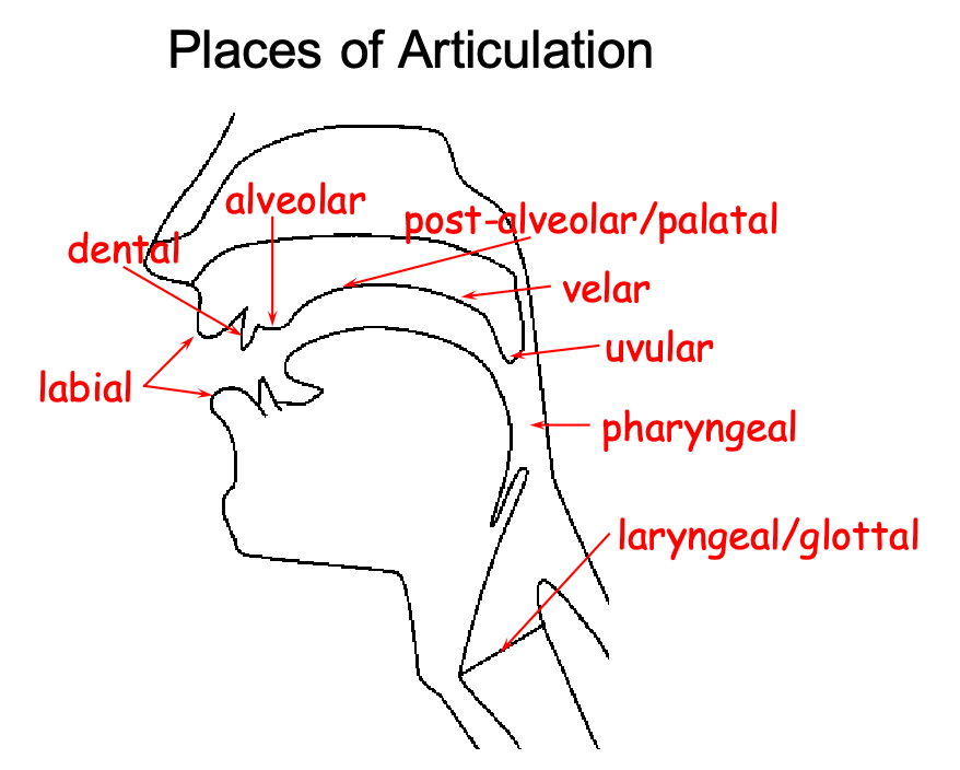
Articulatory Phonetics

How do you produce sounds? Each language is different, but typically multiple parts of your body:

In English, we further have:

• Consonants: voiced or voiceless, but often with restriction/blockage of air flow
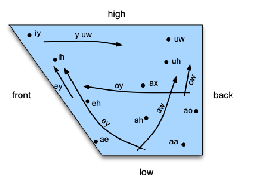
• Vowels: generally voiced with little restrictions. Variations in different vowels caused by factors such as ‘height of tongue’, ‘roundness of lips’

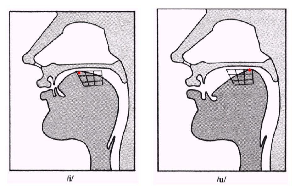
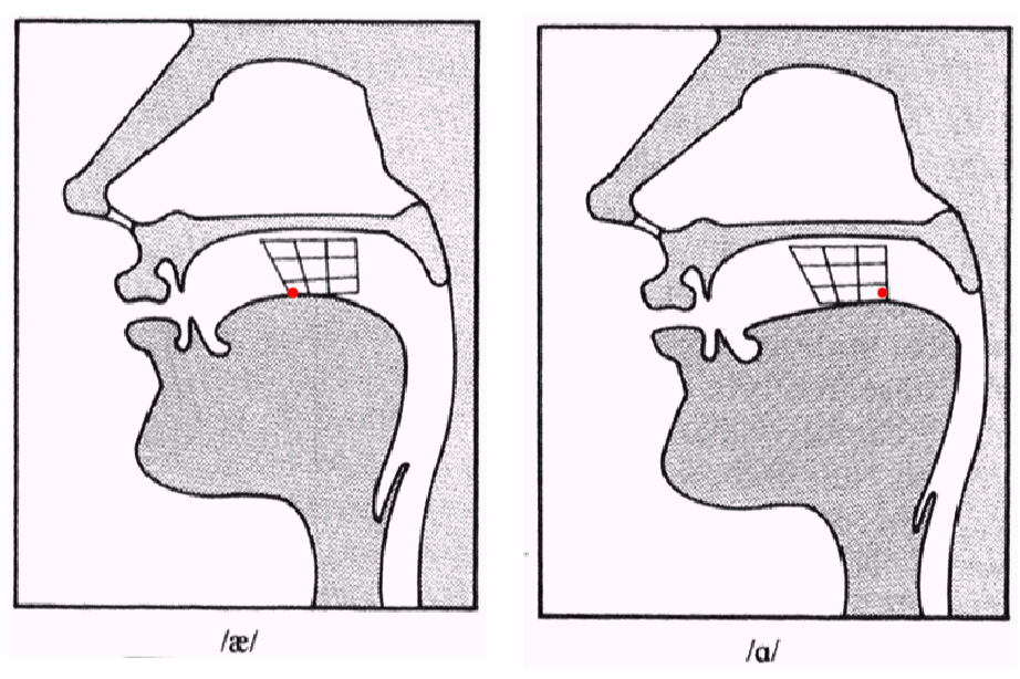
More specifcally, vowels can be categorized into

For example:

High Front or Back for [iy] and [uw]	Low Front or Back [ae] and [aa]

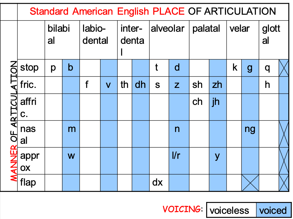
For consonants, two things define its type: place of articulation and manner of articulation

Coarticulation: one challenge is that things can be different depending on its phonetic context - a major issue in ASR

• e.g. place of articulation moves forward in “eight” v.s. “eighth”, due to different adjacent sounds

Representations of Sounds

We have ways to represent sounds (e.g., IPA) and to classify similar sounds. This is important, because it relates to how systems such as ASR, TTS (speech synthesis), Speech Pathology, Language/Speaker ID.

So how do we recognize sounds automatically?

• e.g., use the relationship between representation and acoustics to identify speech automatically?

  

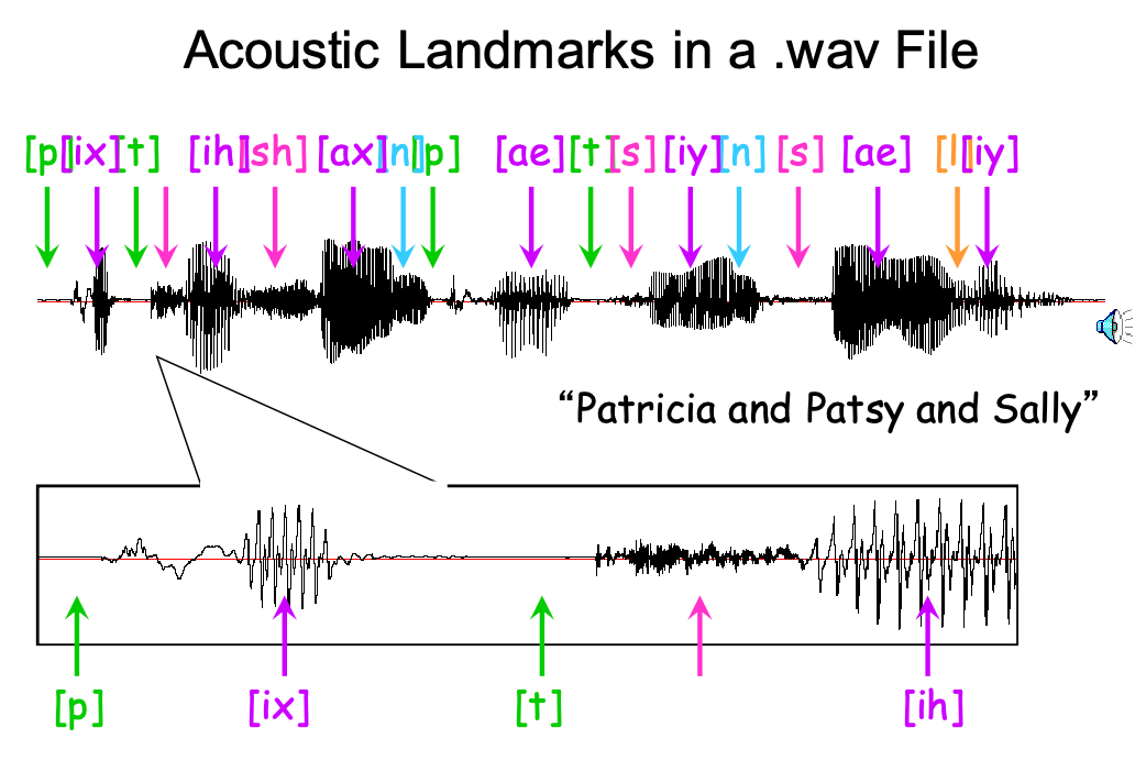
  notice that vowels (purple) have higher amplitudes, and also note that these “shape” will change depending on what is pronounced before them.

• and interestingly, people (Nima Mesgarani) show that you could directly produce speech using brain signals

  

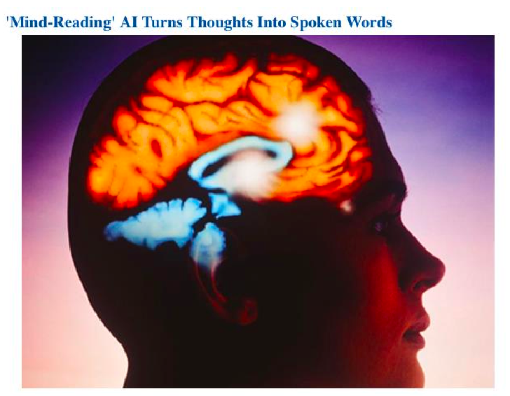
  i.e., think it in your brain and we can identify what you were thinking! (combining speech synthesis and brain interface!)

Reading notes for Lecture 1

Key notes from Jurafsky & Martin Chapter 28 (Chapters 1-3)

• earliest writing systems we know of (Sumerian, Chinese, Mayan) were mainly logographic: one symbol representing a whole word. But

  • some symbols were also used to represent the sounds that made up words

• the idea that the spoken word is composed of smaller units of speech underlies algorithms for both speech recognition (transcribing waveforms into text) and text-to-speech (converting text into waveforms)

  • but the difficulty is that a single letter (e.g., p) can represent very different sounds in different contexts

• Phonetics: the study of the speech sounds

• We will represent the pronunciation of a word as a string of phones (see the transcription part). Examples look like

  

  where the standard representation is using the International Phonetic Alphabet (IPA) symbols, but here we use the ARPAbet as it uses ACSII.

• Articulatory phonetics: how these “phones” are pronounced by various organs in the mouth, throat, and nose

  

  • Consonants are made by restriction or blocking of the airflow in some way, and can be voiced or unvoiced
  • Vowels have less obstruction, are usually voiced, and are generally louder and longer-lasting than consonants.

• More specifics about consonants:

  • can group consonants into their point of maximum restriction, their place of articulation

  • Consonants are also distinguished by how the restriction in airflow is made, for example, by a complete stoppage of air or by a partial blockage

    

    and the combination of how and where is usually sufficient to uniquely identify a consonant.

• More specifics about vowels:

  • The three most relevant parameters for vowels are what is called vowel height, which correlates roughly with the height of the highest part of the tongue

    • vowel frontness or backness, indicating whether this high point is toward the front or back of the oral tract and
    • whether the shape of the lips is rounded or not

    

• Consonants and vowels combine to make a syllable

  • yes, there are rules of what constitutes a syllable, although practically everybody knows by trying to pronounce them

    

    where:

    • initial consonants, if any, are called the onset
    • The rime, or rhyme, is the nucleus (vowel at the core of a syllable) plus coda (optional consonant following the nucleus)

• Prosody is the study of the intonational and rhythmic aspects of language, and in particular the use of F0, energy, and duration to convey pragmatic, affective, or conversation-interactional meanings. On a high level:

  • energy as the acoustic quality that we perceive as loudness
  • F0 as the frequency of the sound that is produced
  • acoustic quality is what we hear as the pitch of an utterance.

  this is heavily used to convey affective meanings like happiness, surprise, or anger. For example, speakers make a word or syllable more salient in English by saying it louder, saying it slower (so it has a longer duration), or by varying F0 during the word, making it higher or more variable

• Prosodic Prominence: Accent, Stress and Schwa

  • Words or syllables that are prominent are said to bear (be associated with) a pitch accent (e.g., the underlined words below):

    “I’m a little surprised to hear it characterized as happy.”

  • syllable that has lexical stress is the one that will be louder or longer if the word is accented. For example, the word surprised is stressed on its second syllable, not its first

• Prosodic Structure: some words seem to group naturally together, while some words seem to have a noticeable break or disjuncture between them.

  • an example we have seen earlier “They city hall parking lot was chock full of cars.”
  • Automatically predicting prosodic boundaries can be important for tasks like TTS

• The tune of an utterance is the rise and fall of its F0 over time.

• A very obvious example of tune is the difference between statements and yes-no questions in English

  a final F0 rise	a final drop in F0 (also called a final fall)

Acoustics of Speech

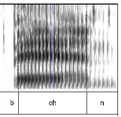
How do we automatically distinguish one pheome from speech, even if they sound similar. For example, how do we distinguish between “kill him” v.s. “bill him” only using sound (e.g., using spectrograms, see Reading notes)

Sound production:

• signal to noise ration (SNR): sound produced might not always be people’s speech
• harmonic to noise ratio (HNR): ratio between periodic and a-periodic speech components. In particular, speech waveform that show repeating patterns over time in distorted or unnatural speech

What do we need to capture good speech data?

• good recording conditions (quite space)
• close-talking microphone (right next to the bottom left of your lips)
• a good microphone that can capture at least 2 samples per cycle (to figure out the frequency)
  • human hearing can discern up to 20k, but for studying speech, typically 16k-22k sampling rate is enough
  • this probably also relates to how humans acuity is lower at higher frequency

Sampling errors:

• aliasing: different signals can become indistinguishable from one another when they are sampled
  • e.g., often happens when sound $>$ nyquitst frequency, or when you quantized too much
  • e.g., solutions include simply increase your sampling rate (or called resolution), or buy larger storage to store more bits per sample
• speech file formats: mostly wav, and a useful tool is SoX (sound eXchange) that can convert between many formats

Frequency:

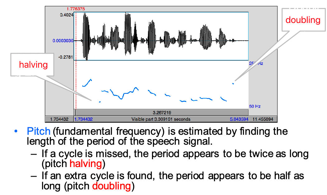
• pitch track: plotting F0 over time

  

• how exactly is F0 determined? by definition: F0 approximate frequency of the (quasi-)periodic structure of voiced speech signals. This means if you zoom into any segment of speech wave, you will see some periodic pattern (originates from our vocal cord):

  

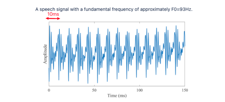
  for exmaple, the F0 above is $F_0 = 1/0.01 \approx 100 \mathrm{Hz}$, where $T\approx 10\mathrm{ms}$ above. Of course, since these are produced by an organ, it’s not exactly periodic and have fluctuations. Specifically, the amount of variation in period length and amplitude are known respectively as jitter and shimmer.

• there are softwares that can automatically plot these, e.g. Praat

  • but note that it can contain errors, such as pitch doubling or halving (i.e., looks very high or low in the diagram, but we don’t perceive it as high)

  

• difference between pitch and F0? Pitch is how human perceives the F0, and humans has lower acuity at higher frequency

  • hence there is stuff like the mel scale to measure frequency (see Reading notes)
  • the dB scale mostly measure **amplitude **(e.g., whisper is about 10dB, normal conversation is about 50-70dB)

How is HNR useful?

• lower HNR indicates more noise in signal, often perceived as hoarseness and roughness (emotionally-wise)
• can also be used to discern pathological voice disorders

More on visualizing waveform:

• fricative v.s. vowel, the latter more clearly articulated

  

• and we can also use libraries to get the spectrogram of a waveform (by doing Fourier transforms) and analyze from there, i.e. using the formants (see Reading notes)

  

  but again, these formants will change depending on the consonant contexts.

• What’s the connection between the fundamental frequency $F_0$, and the formants $F_1, F_2, …$? if we consider a spectrum of a speech segment (i.e., the frequency-amplitude space after Fourier transform):

  

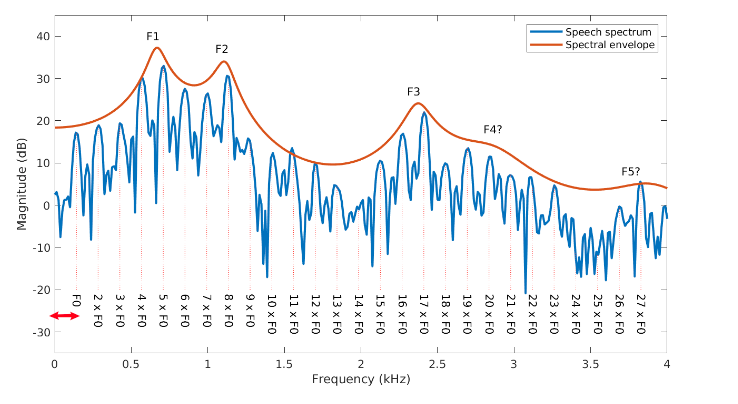
  notice that F1, F2, ... are the frequencies of the amplitude peaks (i.e., the dark spots in the spectrogram), and they are all integer multiples of F0, which can be found by counting how frequent things peak here.

• useful library here include MFCC and Praat, which can basically give you every quantity mentioned above automatically

Reading Notes for Lecture 2

• acoustic analysis is going again back to sine and cosine functions:

  \[y = A * \sin(2\pi ft) = A * \sin(2\pi t / T)\]

  and sound waves are basically the above due to the change in air pressure = compression and rarefaction of air molecules in a plane wave. For example:

  

  how is this produced in reality? It’s an analog-to-digital conversion where:

  1. we sample `$\to$ sampling frequency. To accurately measure a wave, we must have at least two samples in each cycle.
     • this means the maximum measurable frequency is half of the sampling rate. For human speech, we would need 20,000 Hz sampling rate = measure 20,000 amplitudes per second
  2. we quantize real value measurements into integers
     • for easier storage, we sometimes also compress them, e.g., using $\mu$​-law which is a log compression algorithm.

• tie this back to articulatory phonetics:

  • the frequency we record come from vibration of our vocal folds
  • so each major peak in Figure 28.9 corresponds to an opening of the vocal folds

  then basically we are recording frequency of vocal folds vibration , which is called fundamental frequency of a wave form, often abbreviated as F0:

  

  for example, in the middle plot above we show the F0 over time in a pitch track = plotting the frequency as a function of time.

• Similarly we can also plot (average) amplitude variation over time. But since directly averaging them you would get near zero everywhere, people typically use 1) root mean square amplitude 2) normalize it to human auditory threshold, measured in dB.

  \[\mathrm{Intensity} = 10 \log_{10} \frac{1}{NP_0} \sum_{i=1}^N x_i^2\]

  visually:

  

• human perceived pitch relates to frequency, but the difference is that:

  • human hearings has different acuities for different frequencies
  • mostly linear for low frequency below 1000Hz (can accurately distinguish), but logarithmically for high frequency.

  as a result, there is also a mel scale, where a unit of pitch is defined such that pair of sounds which are perceptually equidistant in pitch are separated by an equal number of mels.

• human perceived loudness corelates to power, but again

  • humans have a greater resolution in the lower-power range

• phones can often be visually found by inspecting its waveform:

  

  notice that vowels are often voiced = have regular peaks in amplitudes.

• an alternative representation of the above is to use Fourier analysis to decompose a wave at any time using frequencies and amplitudes of the composite waves:

  Original Wave	Fourier Decomposition

  recall that since Fourier analysis can break any smooth function $f(t)$ into a sum of sine/cosine waves:

  Original Wave	Fourier Decomposition
  	1

  but why is this decomposition useful? It turns out peaks (e.g. around 930, 1860, and 3020Hz) are =characteristics of different phones.

• a yet another way of representing sound is using spectrograms (inspired by the finding above). In a spectrogram, we can plot all time, frequency, and amplitude by using a dark points to signify high amplitude:

  

  this is useful because:

  • let each horizontal dark bar (or spectral peak) be called a formant
  • then F1 (first formant) of the first vowel (left) is at about 470Hz, much lower than the other two (at about 800 Hz)
  • so again, since different vowel have different formants at characteristics places = spectrum can distinguish vowels from each other (typically just using F1 and F2 suffices)

• there are many online phonetic resources where we can use for computation work, here a few is highlighted

  • online pronunciation dictionaries such as LDC
  • phonetically annotated corpus, a collection of waveforms hand-labeled with the corresponding string of phones

Tools for Speech Analysis

Praat: a general purpose speech tool for

• editing, segmentation and labeling sounds
• can also create plots!

Assuming you have already gone through the tutorials (record, analysis, and save). By default, viewing a sound file should also give you a spectrogram

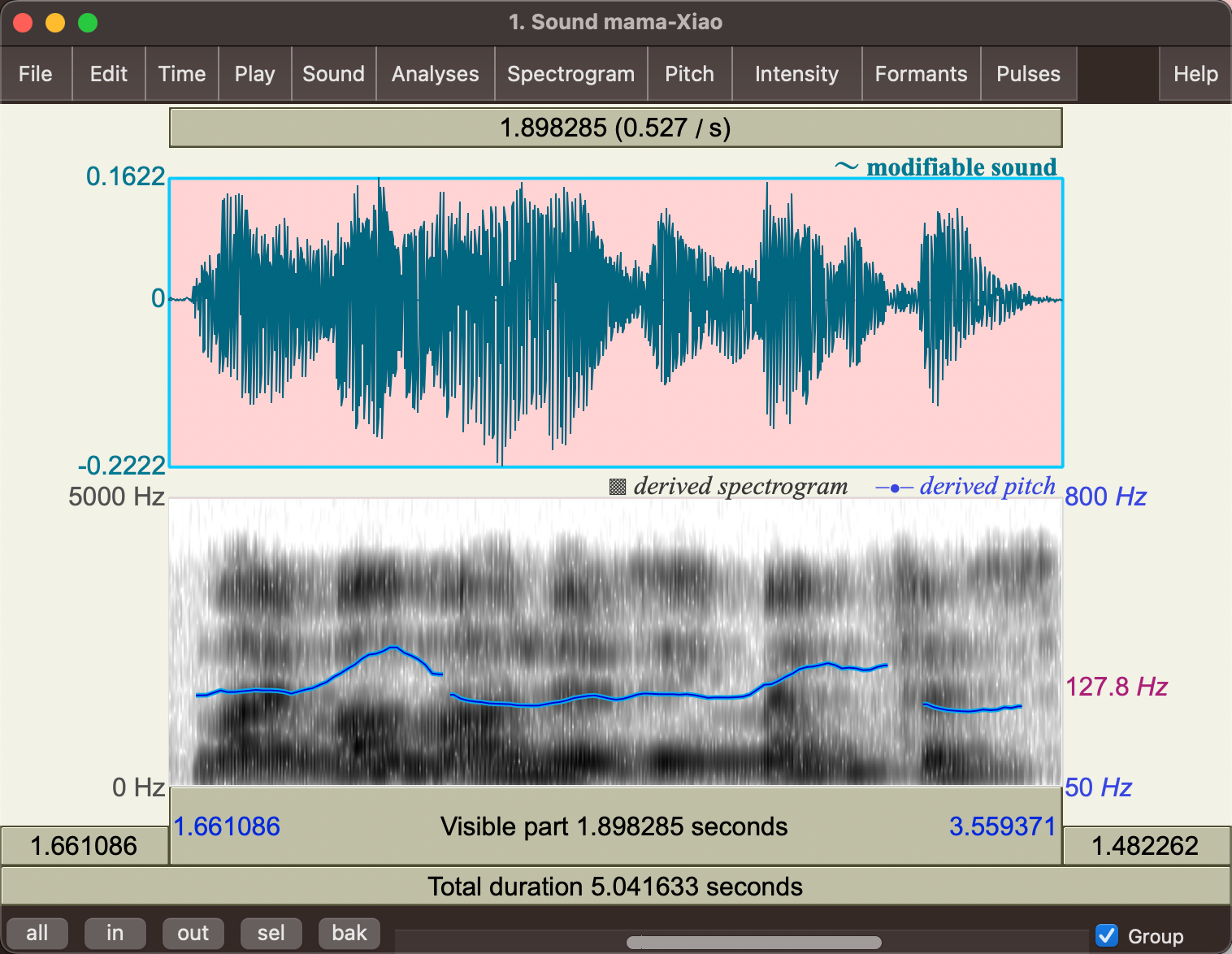
and basically from the top menu bar, you can analyze information such as “maximum pitch”.

By comparing the analysis between different files, you could find:

• maximum pitch of male voice is much lower than that of females
• intensity for whispering is lower than not whispering
• F0 contour rises at the end for yes or no question
• etc.

You can also manipulate your sound using the manipulation option from the objects window. For example, changing the pitch and duration (speed) of the last part of the “My mama lives in Memphis”:

Getting the manipulation object

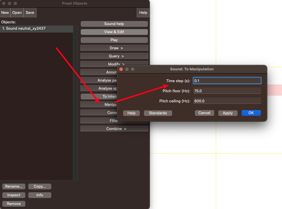Then simply drag and move manipulatable dots using or you can add them (using the menu bar on top)

Normal Sound	Manipulating to get a Y and N question

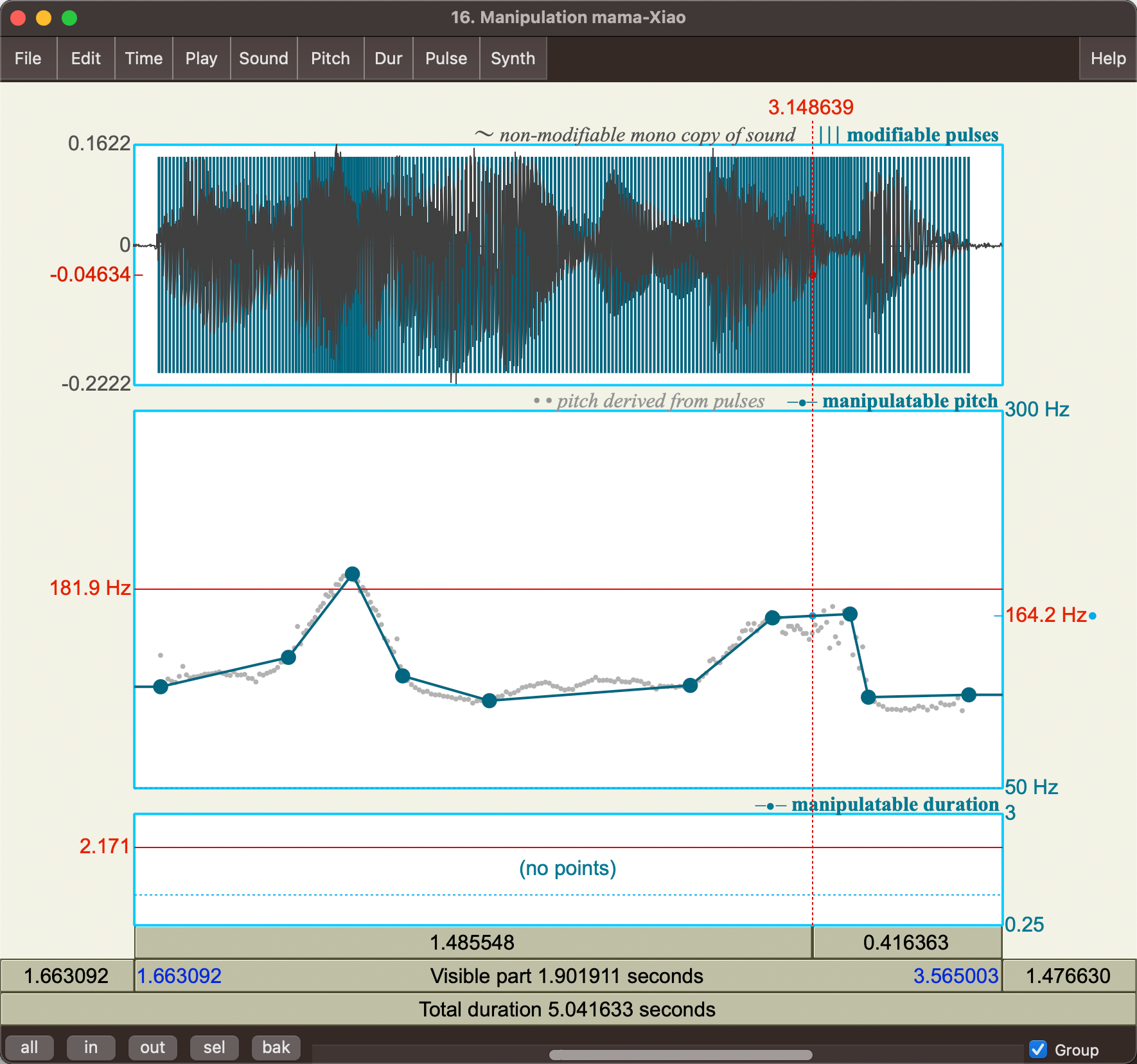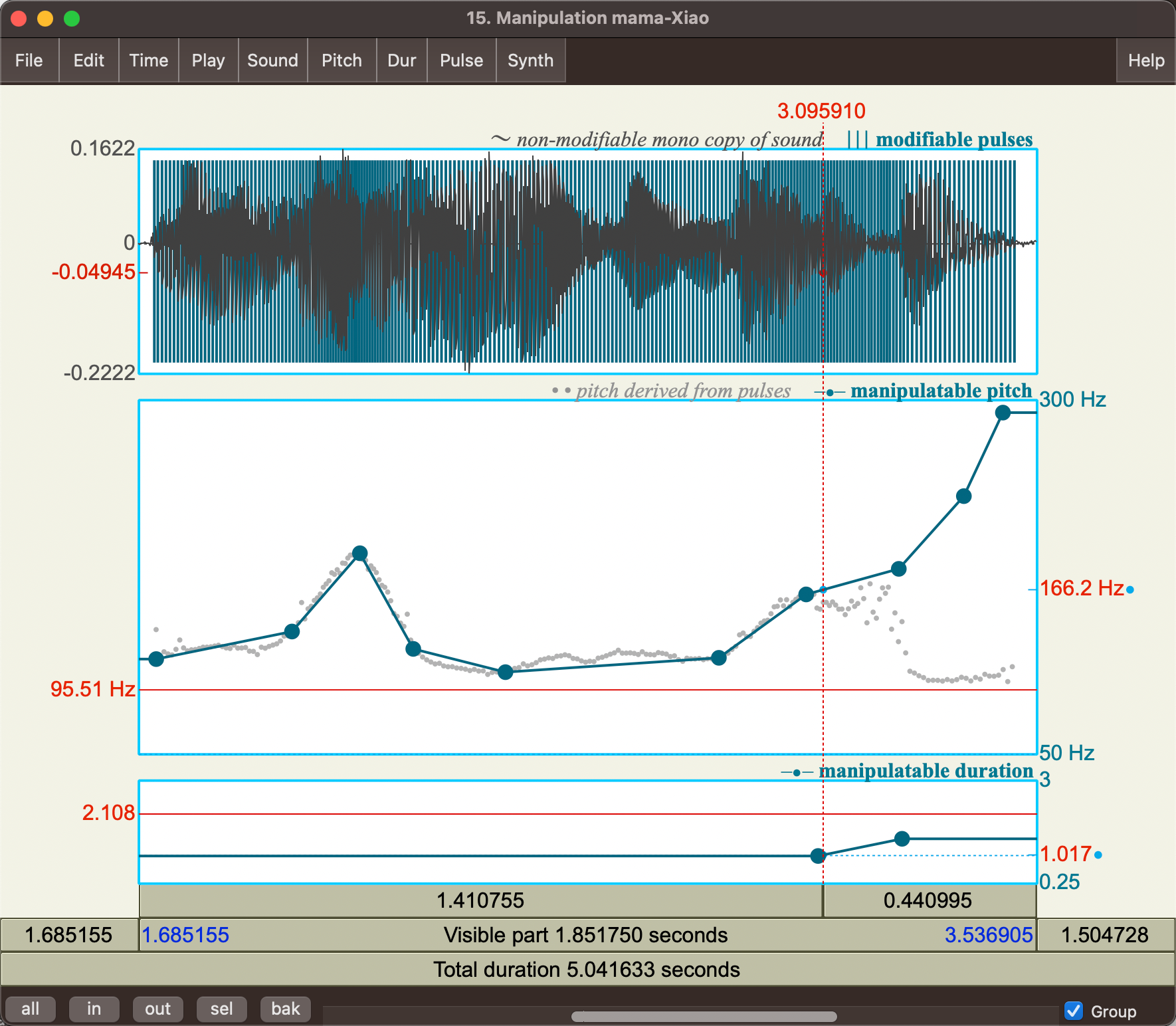For more details, refer to Week 4 on this syllabus: cs.columbia.edu/~julia/courses/CS6998-24/syllabus24.html

Scripting in Praat

The main reference is Sound (uva.nl), but some generic note is you can “translate” clicking in Praat to scripting by, for example:

Obtain mean intensity:

1. Get an intensity object:

   

2. query for intensity min:

   Query Command	Setting/Arguments	Results

The above would translate to the following commands in python. Note that the arguments to the call function are basically the same ones you see in the Settings pop up window above.

import parselmouth
from parselmouth.praat import call

def extract_features_from_file(wav_file_path: str, transcriptions: Dict):
    sound_obj = parselmouth.Sound(wav_file_path)
    data_dict = {}

    ### intensity analysis
    intensity_obj = call(sound_obj, "To Intensity", 100, 0, "yes")
    mean_intensity = call(intensity_obj, "Get mean", 0, 0, "energy")
    max_intensity = call(intensity_obj, "Get maximum", 0, 0, "Parabolic")
    min_intensity = call(intensity_obj, "Get minimum", 0, 0, "Parabolic")
    stdev_intensity = call(intensity_obj, "Get standard deviation", 0, 0)
    data_dict["Mean Intensity"] = mean_intensity
    data_dict["Max Intensity"] = max_intensity
    data_dict["Min Intensity"] = min_intensity
    data_dict["Sd Intensity"] = stdev_intensity
    
    # other code omitted

Analyzing Speech Prosody

Prosody is the study of the elements of speech that aren’t phonetic segments (e.g. vowels and consonants) and is concerned with the way speech sounds.

Differences in how people produce a speech influence how we interpret it (i.e., semantic meanings). Therefore, building a good prosodic model can be very useful for:

• improving text-to-speech synthesis
• improve speech recognition and understanding
• etc.

Some challenges in building a good prosodic model:

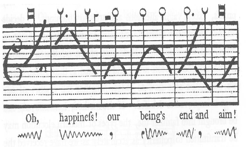
• naively using a pitch contour directly = people could have spoke in different pitches = difficult to represent similarities between contours

  

• how about just annotating them with arrows and capital letters?

  

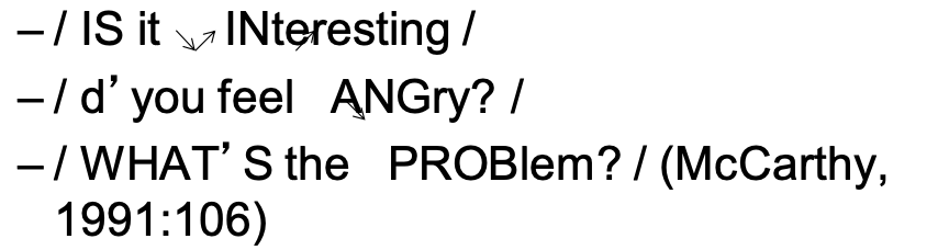
  but this is too generic: it doesn’t capture full contours or type of pitch accents

before we go to modern systems such as TOBI, we need to discusst some definitions

Recall that:

• Prominence/Pitch Accent: making a word or syllable “stand out”
• Perceived Disjuncture: pauses during the speech, for instance used to structure information (e.g., group words into regions)

Tone Sequence Models

How we annotate prosody today:

British School	American School (we will focus on this)

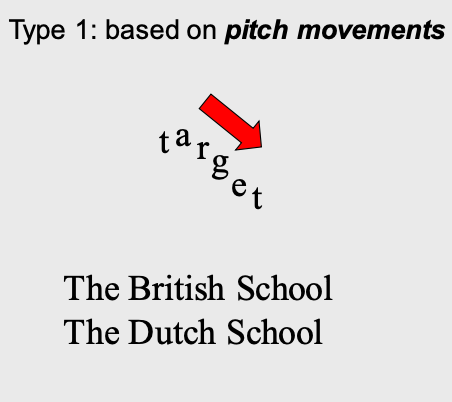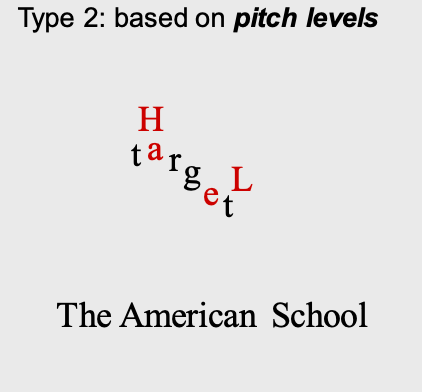On a high level, the American school consider:

• accents (if a particular word is prominent)
• boundary tones (if the entire phrase is prominent)
• phrase accents (if part of a phrase is prominent)
• and different ways to pause (break index), etc.

The American school became popular since the 1980 thesis from Pierrehumbert, where how human produces speech = transitions in the state diagram below:

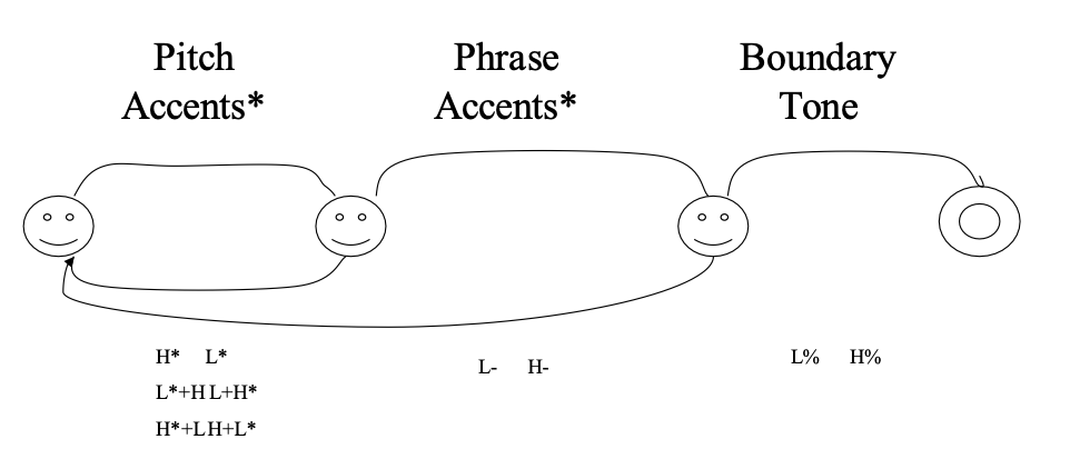
In the 1991-94, there comes the TOBI system that combined the above and other prior work with the goal of

• Devise common labeling scheme for Standard American English that is robust and reliable
• Promote collection of large, prosodically labeled, shareable corpora

In TOBI, prosody is

• inherently categorical in labeling prosody
• basically describes high (H) and low (L) toes associated with events such as pitch accents, phrase accents, and boundary tones
• break indices to describe when you pause, and the degree/length of the pause

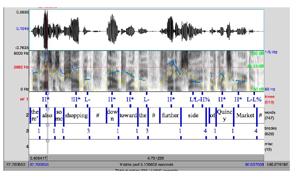
On a high level, TOBI annotates the F0 contour with four tiers:

1. orthographic: annotate the actual words that are said
2. break-index: pauses and how long is the pause
3. Tonal Tier: all accents (prominence) including pitch accents, phrase accents, boundary tones
4. Miscellaneous Tier: disfluencies, laughter, etc.

TOBI Pitch Accent Types

Words can be accented/deaccented in different ways

Accent Contour	Meaning

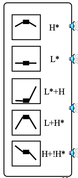An example

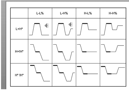
Prosodic Phrase and Phrase Ending in TOBI

Combined we can describe an entire phrase -> combined we can describe accents in an entire sentence.

For instance, the rows indicates the accent to start something, and columns indicate accent in the middle/ending.

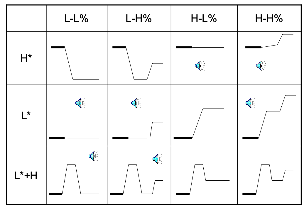
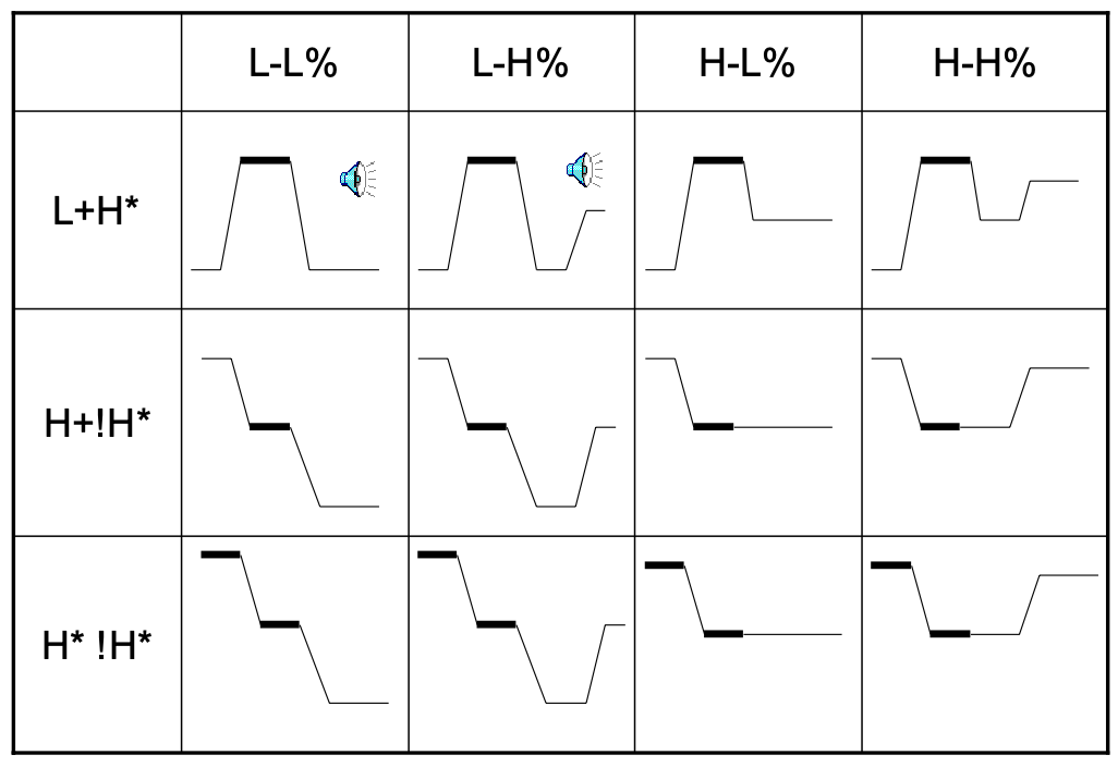
Examples include

• (H*; L-L%) “I (up) like you (down)”
• (L*; L-L%) “Amelia.”
• (L* + H; L - H%) “A (low) me (high) li (low) a (up)”

A full example with a sentence (note that no label for a word = deaccented/no accent)

Although it might seem “subjective” to decide when there is an accent and how its accented, but it turns out:

• 88% agreement on presence/absence of tonal category
• 81% agreement on category label
• 91% agreement on break indices to within 1 level

so after some training this should be pretty robust/intuitive!

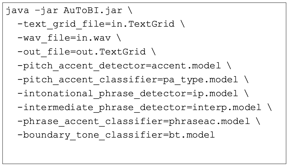
AuTOBI

Somebody also built a way to automatically annotate a voice track with TOBI. Basically it identifies pitch accents and boundaries with high accuracy using many acoustic-prosodic features.

Input you will give:

• Time-aligned word boundaries (human or automatically done)
• a .wav file of the speech
• some previously trained AuToBI models (e.g. for different language, trained on different corpus)

Output

• TOBI tones and break indicies
• confidence scores as well

An example

Other Prosodic Models

There are many other ways to model prosody and analyze them.

• many models are developed for database retrieval, phonological analysis and text-to-speech synthesis
• How can we extract information from large speech corpora that go beyond pitch, intensity, speaking rate?
• How can we analyze the way subjects convey different kinds of information?
• etc.

Reading Notes for Lecture 4

Analyzing Speech Prosody

See PDF at conv.dvi (columbia.edu)

The TOBI (Tones and Break Indices) annotation system is a tool used for marking intonation and prosodic structure in spoken language. TOBI provides a standardized way to annotate speech, facilitating the study of how intonation patterns affect meaning, signal sentence structure, and express speaker attitudes.

It consists of four tiers for labeling the F0 contour of a speech:

1. an orthographic tier

   • an orthographic word = one standalone English word
   • transcription of orthographic words done at the final segment of the word = the right edge
   • some considerations here include: whether or not to annotate pauses such as “er”, “mm”, “uh”, etc.

2. a tone tier: we mark two type of events

   • pitch events associated with intonational boundaries (phrasal tones)
     • assigned at every intermediate phrase
     • L- or H- phrase accent, which occurs at an intermediate phrase boundary
     • L% or H% boundary tone
     • %H high initial boundary tone = phrase that begins relative high in the speaker’s pitch range
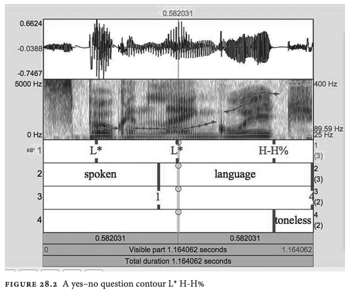
     • example include “H-H%” in a yes-no question, and “L-L%” for a full intonation phrase with a L accent ending its final phrase and a L% boundary tone falling to a point low in pitch
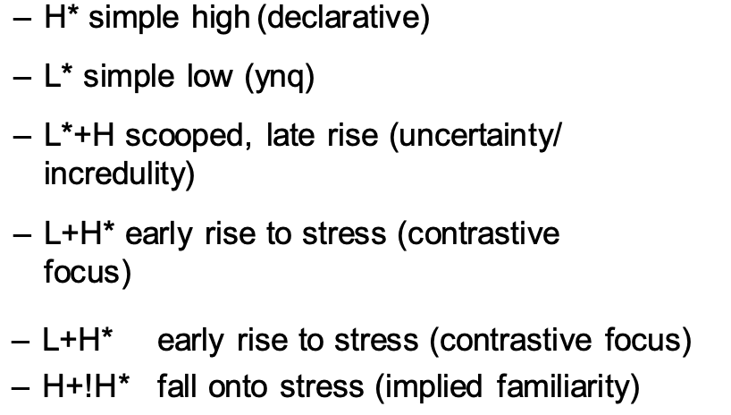
   • pitch events associated with accented syllabus (pitch accent)
     • marked at every accented syllable
     • H* peak accent = high pitch range for the speaker
     • L* low accent
     • L*+H scooped accent = low taget on the accented syllable immediately followed by a sharp rise
     • L+H* rising peak accent = a high peak target on the accented syllable preceded by a sharp rise from a valley
     • H+!H* a clear step down onto the accented syllable…
   • examples include:

   low boundary tone	yes-no question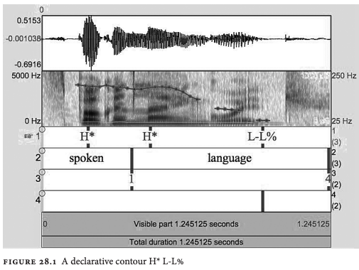

   other variants of phrasal accents are shown in

   

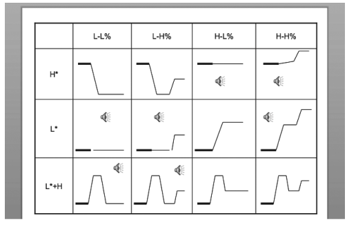
   examples of syllable accents:

   

3. a break-index tier

   • break indices are to be marked at the right edges of words transcribed in the Orthographic tier. All junctures have an explicity break index value.
   • break-index values include:
     • “0” for clear phonetic marks of clitic groups (e.g., “0” between “Did” and “you” indicating palatalization)
     • “1” for most phrase-medial word boundaries (e.g., a mere word boundary between “you” and “want”)
     • “2” strong disjuncture due to a pause
     • “3” intermediate intonation phrase boundary: “a single phrase tone affecting the region from the last pitch accent to the boundary”
     • “4” full intonation phrase boundary (e.g., “4” at the end of a sentence.)
   • (in practice, its frequently “0” = no juncture, “1” normal pauses between words. See section Tone Sequence Models for more example)
   • if you are uncertain, use “-“ (e.g., “2-“ means uncertainty between “2” and “1”)
   • disfluencies are indicated by “p”, meaning an audible hesitation. (e.g., “3p”)

4. a miscellaneous tier, used for comments or markings of laughter, disfluencies, etc.

   • labels should be applied at the temporal beginnings and endings by:

     event< ... event>
     

     for example, a period of laughter plus speech (...) looks like:

     laughter< ... laughter>
     

Pragmatics and Prosody

Variation in prosody (i.e., intonation) can influence the interpretation of languages. This section discusses aspects of prosodic variation (e.g., when and where intonation changes) and pragmatic meaning that have been explored by researchers.

To achieve this, many conventions for describing prosodic variation has been developed = can easily compare across researchers

• continuous descriptions focus on describing the F0 contour
• categorical systems describes prosodic events as tokens from a given inventory of prosodic phenomena. Example include TOBI.

TOBI annotations often have some interpretations:

• H* accents of an accented (prominent) word in a declarative sentence = the accented item is new information
• L+H* accents can be used to produce a sense of contrast
• and more

research on the prosody-syntax interface = can these two affect each other?

• how prosodic phrases divide an utterance into meaningful chunks? Can this aid syntactic parsing?

• useful in resolving syntactic disambiguation, such as:

  VP-attachment: Anna frightened the woman | with the gun (Anna held the gun)
  NP-attachment: Anna frightened | the woman with the gun (the woman held the gun)
  

  While prosodic variation can disambiguate syntactically ambiguous utterances, evidence that it does so reliably is mixed. Speakers often manage to convey the distinctions illustrated above without employing particular prosodic means.

• this relationship exists in many languages

Prosodic prominence and phrasing can also influence the semantic interpretation of utterances.

• signal focus, define the scope of negation, quantification, and modals, and influence the interpretation of presupposition

  DOGS must be carried
  dogs must be CARRIED
  

  being a sign on a British train in 1967 confused people that every trainer should have a dog and carry them.

• reference resolution = pronouns may be interpreted differently depending upon whether they are prominent or not, in varying contexts. For instance:

  John called Bill a Republican and then he insulted him
  John called Bill a Republican and then HE insulted HIM
  

  With both deaccented, the likely referent of he is John and him is Bill, but if both are accented, the preferred referents of each are switched.

Prosodic can indicate some discourse phenomena (i.e., extract meta information from a conversation)

• information - such as focus of attention, topic/comment, theme/rheme, given/new - is often correlated with variation in accent or phrasing

• signaling focus of attention and contrast: not only that prosodic prominence can signal focus but that inappropriate deaccenting of items in focal contexts or accenting of items in non-focal contexts show differences in brain activity in ERP experiments with Dutch speakers.

• conveying information about discourse topic: in task-oriented monologues, speakers referred to local topics with deaccented pronominal expressions, and accented, full NPs otherwise

• distinguishing new/old information: an expression may be prosodically marked as given (i.e., old information) by deaccenting

• convery discourse structure by varying pitch range, pausal duration between phrases, and speaking rate. For instance, it has been found that phrases beginning new topics are begun in a wider pitch range, are preceded by a longer pause, and are louder and slower than other phrases;

• there is considerable evidence that full intonational contours can, in the appropriate context, signal syntactic mood, speech act, belief, or emotion

  • For example, the L*H L-H% contour may convey uncertainty

  A: Did you feed the animals?
  B: I fed the L*+H GOLDFISH L-H% (is that what you meant?)
  

See PDF as cs.columbia.edu/~julia/papers/Chapter_28.pdf

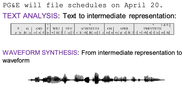
Text-To-Speech Analysis

Requirements for a TTS system:

• Front End: pronounciation modeling; text normalization; intonation

• Backend: waveform production

For example:

And there are many issues and challenges:

• disambiguation in context: “bass”, “reading” (e.g., “Reading is the place he hated most” is pronounced as “reding”)
  • this can be done with Letter-to-Sound Rules or even Pronunciation Dictionary
  • or learn from data
• text normalization issues: “The NAACP just elected a new president.” is pronounced as “N double A CP”
• sentence and phrase break. You think you can just use punctuations, but what about “234-5682”?
  • traditional: hand-built rules
  • current approach: machine learning on large labeled corpus
• assigning pitch contours: in reality no one knows how to assign complex varieties of how human talks
  • e.g., with just “.”’ = declarative contour, wh-question v.s. “?” = yes-no-question contour is doable now
  • but in reality people can put accent everywhere

More on Waveform Generation

They are many types of approaches today:

• (early days) Articulatory Synthesis: Model the actual movements of articulators and acoustics of vocal tract
• (early days) Formant Synthesis: Start with acoustics, create rules/filters to create each formant (i.e., produce formants for each group)
  • the DECtalk system that Stephen Hawking use
• Concatenative Synthesis: Diphone or Unit Selection using databases to store speech segments (i.e., select from database + glue the waveforms)
  • this is actually used a lot in commercial products until late 1990s
  • directly using this produces a speech that is not very smooth. How do we do post-processing on the output?
• Parametric Synthesis: ML-based learning methods
  • used by SIRI in early days
• End2End Models

Concatenative Sythesis

There are two ways to do this:

• diphone synthesis: every sound/unit is a diphone (two phones)
  • all you need is a collection of recording for all possible diphones
  • then you just fetch the diphones and concatenate them to produce speech
  • intelligible, but not very natural/continuous
• unit selection synthesis: use larger units than diphone
  • not only diphone, but also record common ones and common phrases
  • use dynamic programming to search to find best sequence of units, and then concatenate them
  • better than diphone synthesis since you are joining less disjunct chunks

Visually, diphone synthesis could cut at eh and join things:

Example Diphone 1	Example Diphone 1

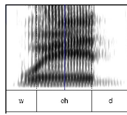For unit synthesis, the challenge is how to find the unit that best matches the desired synthesis specification. What does best mean here?

• Target cost: Find closest match in terms of
  • Phonetic context
  • F0, stress, phrase position
• Join cost: Find best join with neighboring units
  • Matching formants + other spectral characteristics
  • Matching energy
  • Matching F0

and more. The end goal is to get a better prosody selection. However, this is good only when the database is large and diverse enough:

• This has bad performance when no good match in database
• Hard to control the overall prosody/vary speaker identity

Parametric Synthesis

The idea is to use ML to generate acoustic features:

• Hidden Markov Model Synthesis (good in the early days)
  • predict the acoustic property of each phone in each context
  • a best non-neural parametric system
• Neural Net Synthesis (many modern TTS systems)
  • can capture more complex relationships
  • began to overcome naturalness issues

An example of NN systhesis approach:Merlin and Neural Net Synthesis: use NN to predict acoustic features, and use a backend to generate waveforms

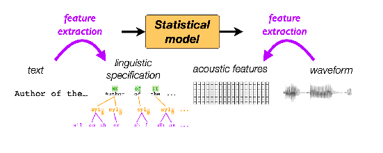
• features for each phone include: “Current phone; Surrounding phones; Position in syllable/word/sentence; Stress; …”
• so this NN is only doing the frontend. It is not an end-to-end model.

Problem: not end-to-end means error can accumulate!

End-to-End Models

Directly generate waveforms from text:

• even more natural, and used in many TTS systems today

• but also require a lot of training data

• examples include WaveNet (based on CNN), Tacrotron (based on Transformer)

  

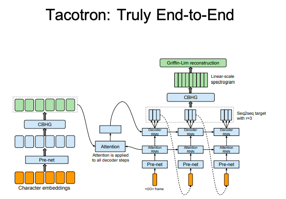
But why was Tacrotron so good?

• Autoregression is very useful: each new waveform is conditioned on previous context
• Neural nets are mostly better at learning contextual features
• Attention mechanism: Only minor improvements

Problems with this approach:

• losing low-level control as we let the model do everything
• need large data and large model

Producing Trustworthy Voices

The second part of the lecture was about how to produce trustworthy speech, and how human perceive trustworthiness in speech.

Some studies that does this include synthesizing speech + putting online survey to have people rate them

• use STRAIGHT toolkit in Matlab, which allows you to manipulate sound
• specifically considered speech stimulus in 5 parameters:
  • F0, frequency, spectro-temporal density, aperiodicity
• manipulate and combine parameters
• only focus on the producing the word: “hello”

Some interesting results found were:

Overall Features	Red is rated as more trustworthy

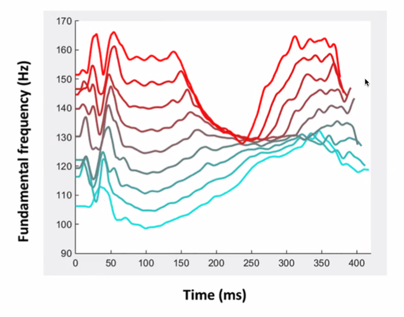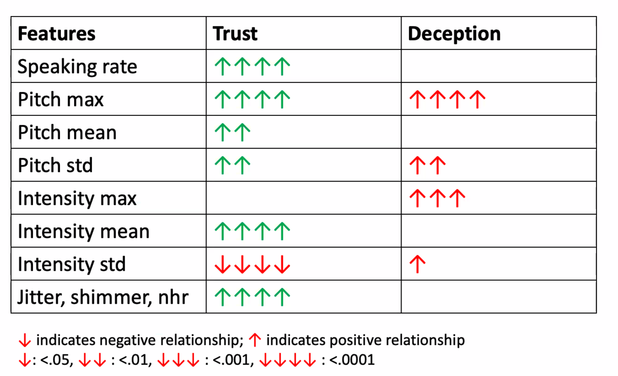
The more latest approach is that you can SOTA TTS model (Amazon Polly) + voice manipulation (Generating Speech from SSML Documents) and meausure longer speeches:

High level features	Lower level features

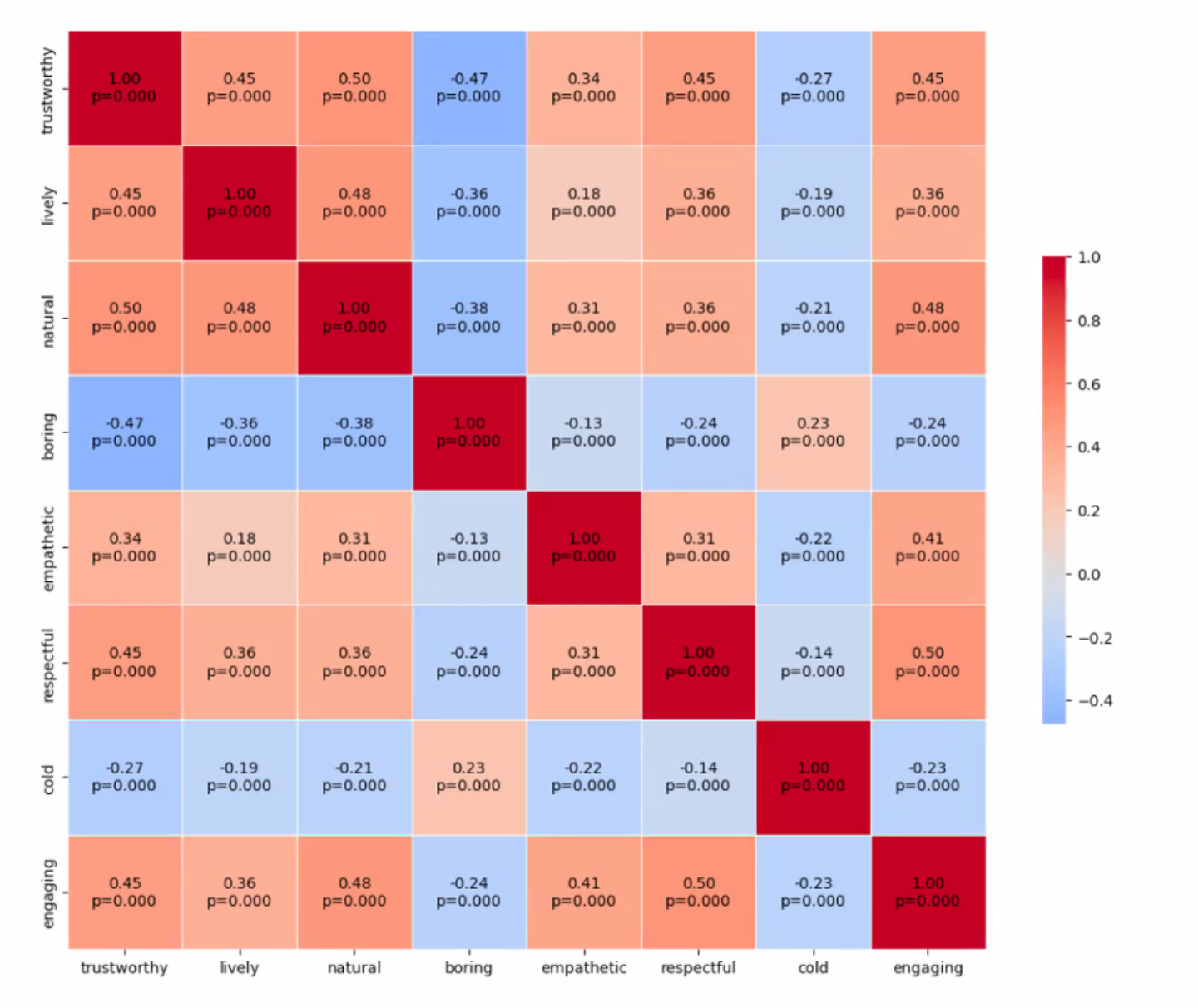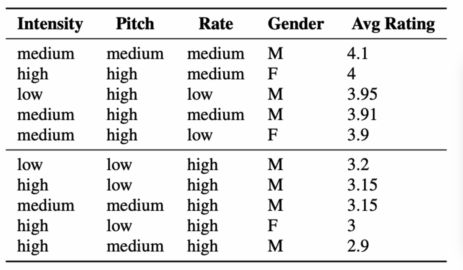where here, they found that trustworthiness (first column) correlates with mostly positive traits such as “engaging and lively”, and that speaking at a lower rate can make you sound more trustworthy.

Speech Recognition

The task of automatic speech recognition is to map waveform to texts

Wave form Input	Text Output

Multilingual modeling for SR today = how can you take a model that is strong in one language/resource, and share/transfer these representations to other tasks and languages?

Some challenges in this area:

• code switching: speaker switches between languages within a single utterance (phrase)
  • relates to language identification task (LID) mentioned below (Reading Notes for Lecture 6)
  • need to cater to different dialects as well
• ambiguity in transcription: there may be more than one way to write the same said phrase in some languages = can artificially inflate WER.
  • need to differentiate modeling error (actual errors) and render error (wrong language due to code switching)
  • some attempts: map all the transcribed words and reference into a single language space

Code-switching has been a “pain” and yet so practical that there are many attempts includeing

• data augmentation: synthesize code-switching utterances

  • some great datasets to begin with FLEURS: Few-shot Learning Evaluation of Universal Representations of Speech (arxiv.org)

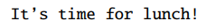
  • pretraining with unlabled speech, as well as incorporating multimodal data (primarily unspoken speech = text) Google USM: Scaling Automatic Speech Recognition Beyond 100 Languages (arxiv.org)

    

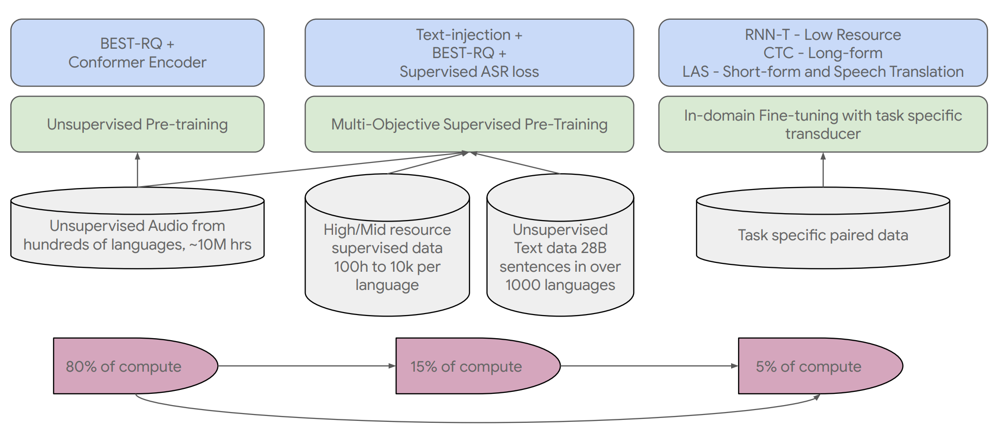
    where BEST-RQ means BERT-based Speech pre-Training with Random Projection Quantizer. The idea is to predict random numbers that correspond to the masked waveform section, as long as the masked-to-random-number-mapping is consistent across different speech segments

    

  • in fact, the idea of modality matching (from non-speech domains) to improve speech models has been quite popular MAESTRO: Matched Speech Text Representations through Modality Matching (arxiv.org)

• other training techniques: constraint the representations of same word different language to be close together

• other modeling techniques:

  • mixture of expert. For each language cluster (e.g., english, spanish, german, etc as one cluster, and Japanese, Chinese, Korean, … in the second cluster, etc.) train a model.
  • language-agnostic approach: transliterate all languages into the same script (e.g. Latin), do inference, and translate back
  • language-dependent approach: just model everything end-to-end

Some key findings:

• shared model representation useful for different languages
• shared data modalities useful for improving ASR and TTS tasks (since these two tasks are like “inverse” of each other!)

How does different kind of data affect the different abilities.

Reading Notes for Lecture 6

• modern ASR tasks vary in different dimensions in practice
  • vocabulary size: standard system involve vocabularies up to 60,000 words
  • recognizing read speech (e.g., audio books) is different from conversational speech
  • whether its recorded in a quiet room or in a noisy environment
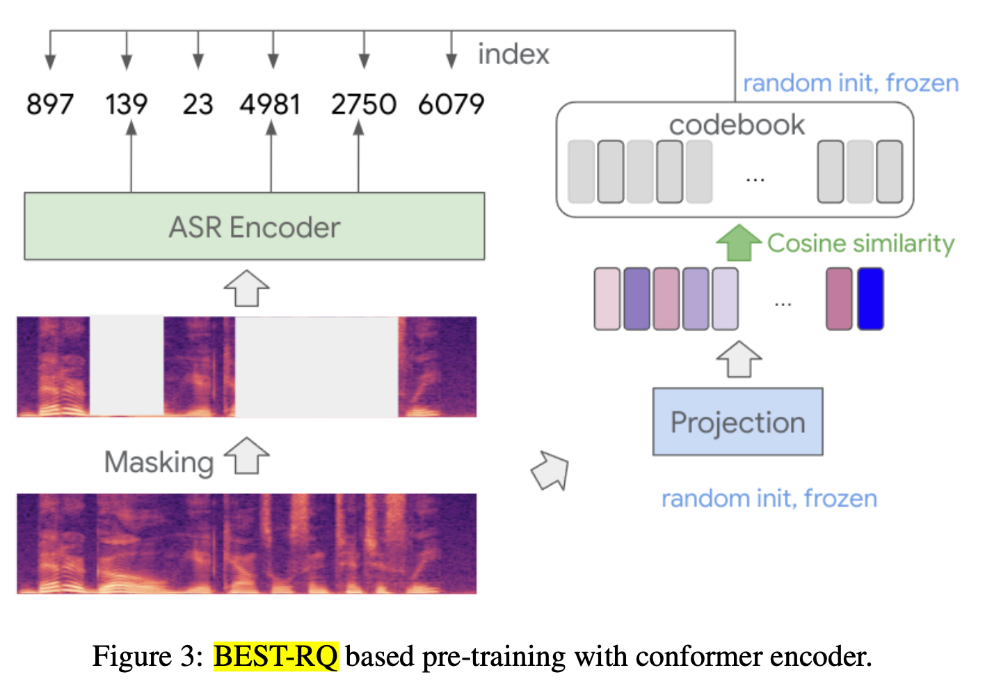
  • speaker identity: dialects, languages, etc. to illustrate the difficulties, modern ASR systems already have a very low word error rate for read speech, but can still have high errors for conversational speech:

  

• examples of modern large scale speech datasets include
  • LibriSpeech: 1000 hours of read English speech
  • Switchboard: 2430 conversations averaging 6 minutes each
  • etc.
• so how do we do ASR?
  1. feature extraction: log mel spectrum. First we want to transform the waveform into a sequence of acoustic feature vectors.
     • first we slice the waveform into frames (e.g., periods of 25ms)
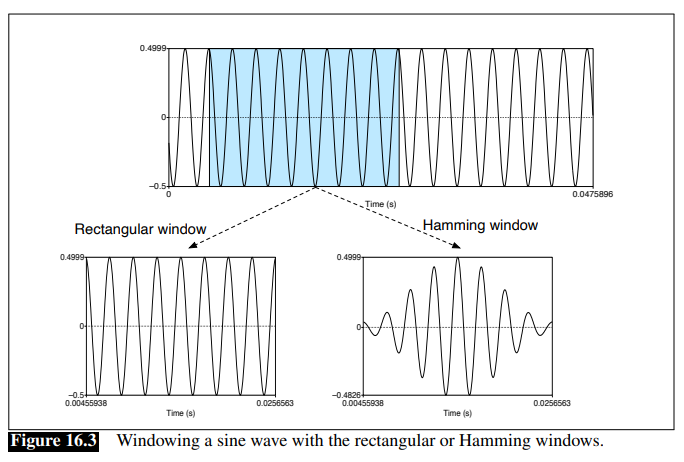
     • you may naively use a rectangular window, but in practice people use Hamming window since the former will create problems with Fourier transform

     Framing	Hemming Window vs Rec Window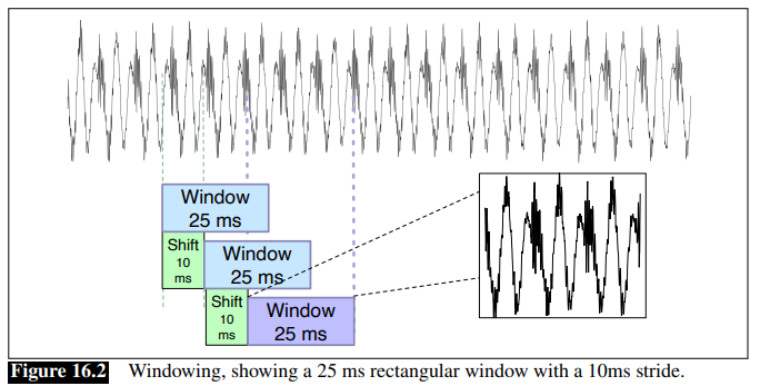

  2. extract spectral information using Discrete Fourier Transform (DFT)
     • take each of the windowed signal, and transform it to obtain a spectrum of frequencies:
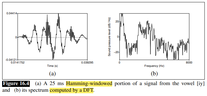
     • this is useful because it tells us approximately the anergy at each frequency band
  3. since human hearing is less sensitive at high frequencies, we can use mel scale to transform the spectrum into a mel spectrum
     • this is done by using a mel filter bank to transform the spectrum into a mel spectrum
     • then you take the log
  4. finally, this sequence of log mel spectral features are used as input to the ASR system
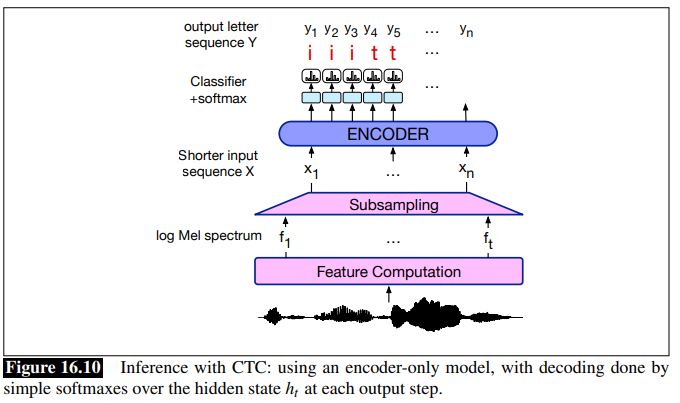
• what model architectures for ASR?
  • typical encoder-decoder models (e.g. with transformers)
  • for example, the system below takes in a sequence of $t$ acoustic feature vectors $f_1, …, f_t$, each being a 10ms frame. Then, the output will be a sequence of letters/word pieces (done by a decoder)
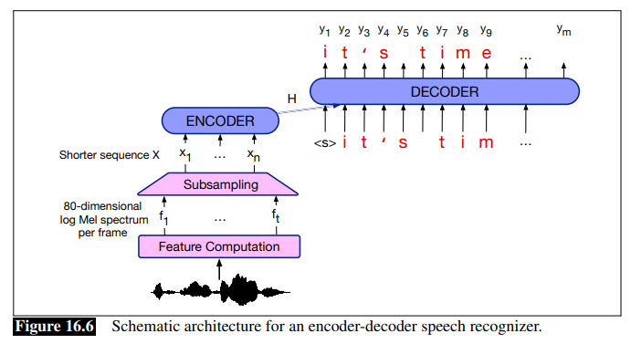
  • however, as shown above a single, 5 characters long word might have 200 acoustic frames, often there is a special compression stage to shorten the feature sequence, denoted as subsampling above.
  • another common practice is to augment the system with an LLM. Since large scale pretraining ASR data is much smaller than pure text, people do 1) use ASR to produce many candidate sequences, and 2) use LLM to rescore them.
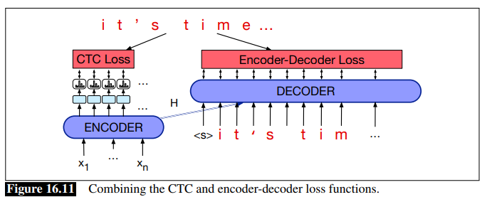
• besides encoder-decoder, another very important algorithm and loss function is called Connectionist Temporal Classification (CTC)

  • idea: output a single character for every frame of the input, but post-process them afterwards by collapsing identical letters. An naive example:

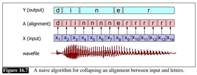
    where the intent was to say “dinner”, but a naive de-dup algorithm would produce “diner”.

  • the smart part of CTC is to add a special blank token:

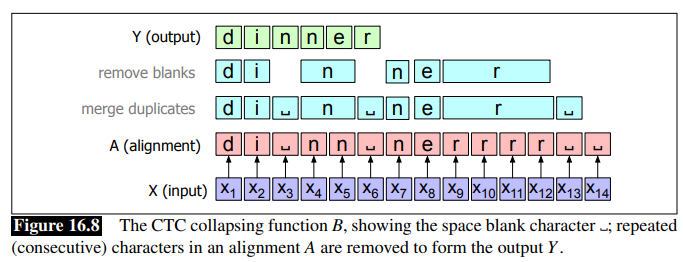
  • but note that this algorithm means there can be many different alignments that produce the same output. This will also be used to formalize how we algorithmically compute the loss function/inference for CTC.

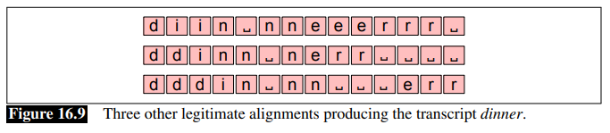
• CTC inference: first we find the best alignment by assuming that each frame is independent to each other (notice that this is different from LM):

  \[P_{\mathrm{CTC}}(A|X) = \prod_{t=1}^{T} P(a_t|X)\]

  where $A = { a_1, …, a_n}$ is an alignment for the input $X$ and output $Y$. Based on this formulation, the best alignment will be:

  \[a_{t} = \arg \max_{a_t} P(a_t|X)\]

  at the end of the day this can be implementing with a traditional encoder LM:

  • but this has a problem: the most likely alignment is not necessarily the most likely output sequence.

  • in fact, the most probable output sequence is the highest sum over probability of all possible alignments:

    \[P_{\mathrm{CTC}}(Y|X) = \sum_{A \in \mathcal{A}(X, Y)} P(A|X) = \sum_{A \in \mathcal{A}(X, Y)} \prod_{t=1}^{T} P(a_t|X)\]

    so it is actually:

    \[\hat{Y} = \arg \max_{Y} P_{\mathrm{CTC}}(Y|X)\]

    which is very expensive to do, and in practice this is approximated using Viterbi beam search.

• CTC loss function using the above, we can formalize a loss function as:

  \[\mathcal{L}_{\mathrm{CTC}}(X, Y) = - \log P_{\mathrm{CTC}}(Y|X)\]

  but since $P_{\mathrm{CTC}}(Y\vert X)$ is expensive as it needs all alignments, we can approximate it with the forward-backward algorithm.

  In reality, people often combine this with the traditional LM loss, and you end up with a CTC+LM loss and an model training that looks like:

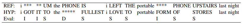
• ASR Evaluation: word error rate: how much the word string returned by the recognizer (the hypothesized word string) differs from a reference transcription
  1. first, compute the minimum edit distance between the two strings

  2. compute word error rate as:

     \[\text{Word Error Rate} = 100 \times \frac{\text{Insertions} + \text{Substitutions} + \text{Deletions}}{\text{Total Words in Ground Truth}}\]

     for example, the following made 6, 3, 1 errors in insertion, substitution, and deletion, and the total number of words in the ground truth is 13, so the WER is 76.9%:

• other speech tasks beyond ASR and TTS include:
  • wake word detection: e.g., “Hey Siri”, but you want to maintain privacy
  • speech translation (ST): conversational spoken phrases are instantly translated and spoken aloud in a second language
  • speaker identification: e.g., “who is speaking?”
  • speaker diarization: e.g., “who is speaking when?”

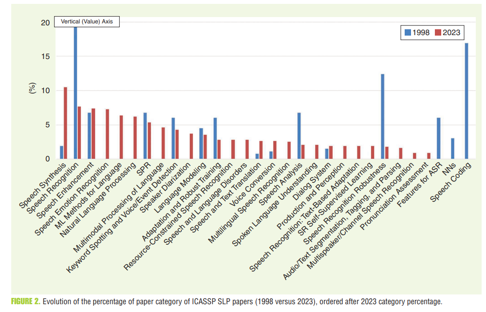
Twenty-Five Years of Evolution in Speech and Language Processing

• overview of the Speech Language Processing field
  • speech coding task: compress speech signals for efficient transmission
  • ASR and TTS: mostly data-driven today
  • speech enhancement and separation: remove noise from speech
• main driving forces in SLP over the last decade
  • big data: it was estimated that 2.5 quintillion bytes of data would be created every day in 2022
  • big, pretrained models: transformer-based models gathered a lot of attention, and self- or semi-self supervised methods used to pretrain many speech models.
• major technical breakthroughs
  • ASR: encoder-decoder models, CTC, and attempts at self-supervised learning methods for speech models
  • TTS: a combination of WaveNet-based vocoder and encoder-decoder models achieved near-human-level synthetic speech, and recently some non-autoregressive models have been proposed to show better performance
• current and future trend:

Spoken Dialogue Systems

some downstream research and applications in spoken dialogue systems

Empathetic Conversations in Dialogue Systems

What is emphay

• cognitive emphasis: “perspective-taking” or being to put yourself into someone else’s place (useful skill for managers)
• emotional empathy: being able to feel other peoples emotions (e.g., you get sad if your friend is sad)
• compassionate empathy: feeling someone’s pain and taking action to help mitigate their problems

Why is this useful?

• empathetic robots = encourage users to like the agents more
• think the agents are more intelligent = more willing to take their advice
• help establish social bonds, promote or diffuse conflict, persuade, succeed in negotiations, etc.
• etc.

some models used:

• speechT5, OpenAI TTS, ElevenLabs, Suno/Bark, meta’s AudioBox for text to speech
• MetaVoice: voice cloning (speak things in some speaker’s style)
• wave2vec for intermediate representation used for classification task (e.g., emotion classification)
• whisper for speech to text

Reading Notes for Lecture 7

Chatbots & Dialogue Systems from the textbook

• Properties of Human Conversation

  • each utterance in a dialogue is a kind of action being performed by the speaker = dialogue acts
  • Speakers do this by grounding each other’s utterances.
  • have structures such as Q and A, sub-dialogues, and clarification questions
  • speakers take turn to have conversational initiative
  • conversational implicature: speaker seems to expect the hearer to draw certain inferences; in other words, the speaker is communicating more information than seems to be present in the uttered words

• chatbots

  • ELIZA and PARRY: rule based systems

  • GUS: Simple Frame-based Dialogue Systems serving as a prototype for task-based dialogue.

    • frames. A frame is a kind of knowledge structure representing the kinds of intentions the system can extract. Basically a collection of key, value pairs, constituting a domain ontology.

      

    • so the goal was to get these slots filled by asking the relevant questions. Some challenges: an utterance may touch multiple slots.

    • domain/intent classification, and extractive slot filling

RASwDA: Re-Aligned Switchboard Dialog Act Corpus for Dialog Act Prediction in Conversations

• The Switchboard Dialog Act (SwDA) corpus has been widely used for dialog act prediction and generation tasks. However, due to misalignment between the text and speech data in this corpus, models incorporating prosodic information have shown poor performance.

  • this transcripts and speech was originally aligned using a GMM-HMM speech recognition system.
  • However, these alignment results are unreliable, making it extremely difficult to use both speech and text data to accurately predict or generate DAs.
  • for example, they have found 27 conversations in which speakers were recorded on the wrong channel, resulting in incorrect speaker identifications

• In this paper, they report the misalignment issues present in the SwDA corpus caused by previous automatic alignment methods and introduce a re-aligned, improved version called RASwDA

  • there are large scale text data annotated with DA, but only a few have been transcribed in speech.

• To produce high-quality alignments between the audio and transcripts of SwDA, we employ a two-step process.

  1. obtain the text grid of each speech file. Since both transcripts and speech spectrogram is there, they then used aeneas library to do automatic alignment
  2. we manually correct the TextGrids produced both from the NXT-format Switchboard Corpus alignments and the aeneas forced alignments

  with this re-aligned corpus, they show that you can have a higher DA classification performance after training.

Nora the Empathetic Psychologist

• Nora is a new dialog system that mimics a conversation with a psychologist by screening for stress, anxiety, and depression as she understands, emphasizes, and adapts to the user.

  • capable of recognizing stress, emotions, personality, and sentiment from speech
  • included an emotional intelligence (EI) module is incorporated to enable emotion understanding, empathy, and adaptation to users

• system design

  

  • empathetic dialog system that takes audio and facial image of the user as input, and basically consists of a) ASR and TTS modules from prior work, 2) empathic module, and 3) a mixed-initiative (text) dialogue system
  • the key new component is this emphathic module, which consists of four submodules
    • stress detection from audio: detect stress from spoken utterances by training on Natural Stress Emotion corpus
    • Automatic emotion detection from audio: another CNN trained with emotion detection dset (6 labels)
    • sentiment analysis
    • personality analysis
  • most models are trained by processing wave spectrograms using CNNs.

Speech Analysis: Emotion Detection and Solicitation

Downstream application of speech analysis.

Emotion and Sentiment Detection

• has many downstream tasks,

• some findings and prior work in emotional recognition

  

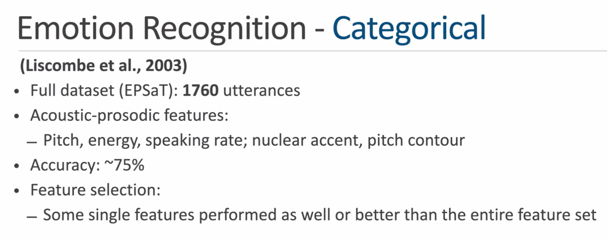
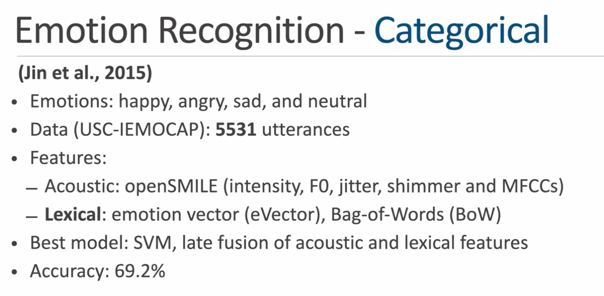
  lexical feature is important:

  

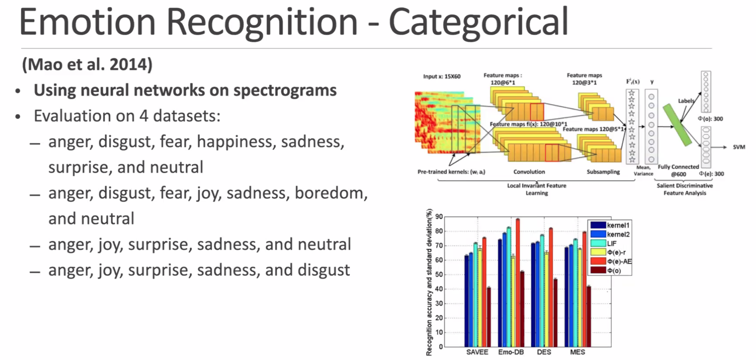
  CNN is strong enough to learn from raw spectrogram and understand emotions

  

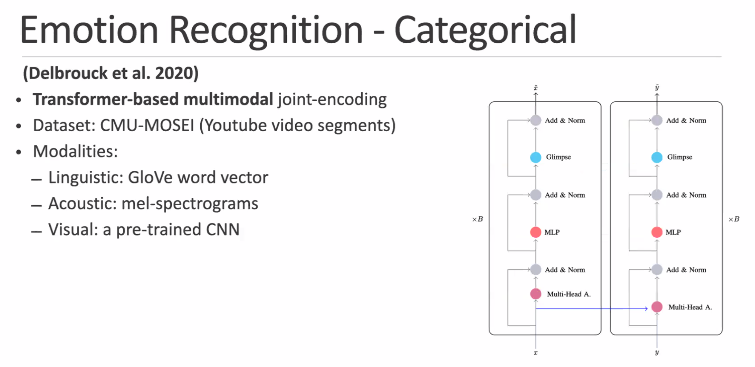
  transformers + multimodal data are great as well

  

Emotion Elicitation

Reading Notes for Lecture 8

Predicting Arousal and Valence from Waveforms and Spectrograms using Deep Neural Networks

• task: Automatic recognition of spontaneous emotion in conversational speech

  • idea: by exploiting waveforms and spectrograms as input, and use CNN to capture spectral information with Bi-LSTM to capture temporal information

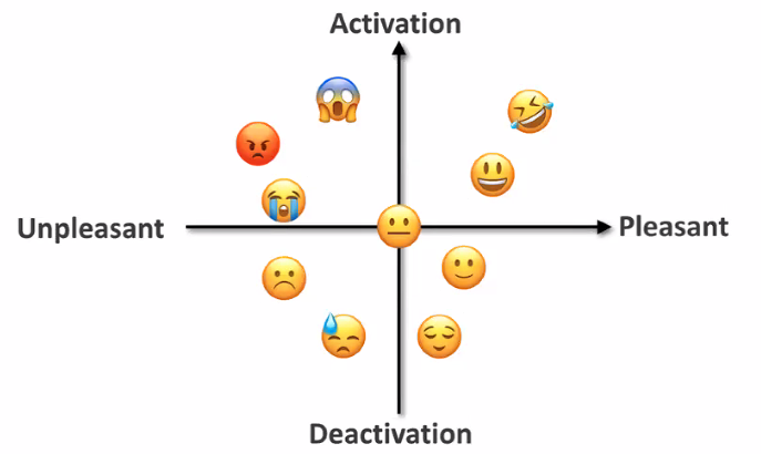
  • instead of classifying into a few emotion cases, map it into a continuous multi-dimensional space (valence-arousal)

    

  • significantly outperforms model using hand-engineered features

• datasets include

  • SEMAINE database: The user’s emotion is annotated by 6-8 annotators for arousal and valence at 20ms intervals
  • RECOLA database: Conversations were annotated for arousal and valence at 40ms intervals by 6 annotators; scores range from -1 to 1 with 2 decimal places

• proposed model architecture: output of CNN layers are then concatenated together for BiLSTM.

  

  but since things are continuous, what does the input really look like?

  • waveform: we normalize waveform signals on the conversation level with zero mean and unit variance to reduce the inter-speaker difference. Then we re-sample the speech to 16kHz sampling rate, and segment the conversation into 6s segments
  • spectrogram: a 40-dimensional mel-scale log filter bank as the spectrogram features. Similar with our preprocessing of waveforms, we first perform normalization and segmentation.

• how do you then measure performance? MSE from the ground truth:

  Arousal	Valence

Emotions and Types of Emotional Responses

• Understanding emotions can help us navigate life with greater ease and stability.
• what are emotions?
  • emotions are complex psychological states that involve three distinct components: a subjective experience, a physiological response, and a behavioral or expressive response.
  • Subjective Experience: experiencing emotion can be highly subjective = what you feel internally differs
  • Physiological response: e.g., your stomach lurch from anxiety or your heart palpate with fear, you’ve already experienced the strong physiological reactions that can occur with emotions
    • early research believes these are mostly due to the sympathetic nervous system, a branch of the autonomic nervous system.
    • but recent research has targeted the brain’s role in emotions. Brain scans have shown that the amygdala, part of the limbic system, plays an important role in emotion and fear in particular.
  • Behavioral response: the actual expression of emotion.
    • ability to accurately understand these expressions is tied to what psychologists call emotional intelligence
    • sociocultral norms also play a role: Western cultures tend to value and promote high-arousal emotions (fear, excitement, distress) whereas Eastern cultures typically value and prefer low-arousal emotions (calmness, serenity, peace).
  • “evolutionary theory of emotion”: emotions are adaptive to our environment and improve our chances of survival
• what kind of emotions do we have?
  • Paul Ekman defined six basic emotions universal throughout human cultures: fear, disgust, anger, surprise, joy, and sadness.
  • Robert Plutchik defined wheel of emotions: how different emotions can be combined or mixed together
• primary vs secondary emotion
  • Primary emotions are the emotions that humans experience universally (e.g., happiness, sadness, fear, disgust, anger, and surprise)
  • Sometimes, we have secondary emotions in response to our primary emotions (i.e., “I’m frustrated that I’m so sad”).
• emotions, feelings, and moods
  • Emotions are reactions to stimuli, but feelings are what we experience as a result of emotions. Emotions are also likely to have a definite and identifiable cause. Feelings are influenced by our perception of the situation
  • A mood can be described as a temporary emotional state. For example, you might find yourself feeling gloomy for several days without any clear, identifiable reason.

Eliciting Rich Positive Emotions in Dialogue Generation

• task: evoking positive emotion state in human users in open-domain dialogue
  • prior work simply aim to “elicit positive emotions”. here they consider more fine-grained emotions such as “Hopeful”, “Joy” and “Surprise”.
  • idea: represent the elicited emotions using latent variables in order to take full advantage of the large-scale unannotated datasets

• prior work: EmpDG

  • EmpDG extracts implicit information from the next utterance as feedback for semantic and emotional guidance of targeted response. These are then used to enhance the base generator model
  • problem? the extracted feedback can be sparse and noisy, which introduces uncertainty in empathetic generation

  

• this work then trains a CVAE network using some pretrained emotion classifier in a GAN-like setting.

Speech Analysis: Entrainment and Code Switching

Entrainment: speakers start to mimic each other’s speaking style as conversation continues.

Code-switching: a person changing languages or dialects throughout a single conversation and sometimes even over the course of a single sentence.

Some findings on conversation with code-switching:

• lexical entrainment exists: similar vocabularies
• acoustic-prosodic entrainment: correlations on stuff like intensity, HNR, etc.
• code-switching behavior entrainment:
  • turn-level synchrony: if I switch language after one turn, the other is likely to switch as well
  • amount of code-switching: if I switch language very often, the other will switch often as well

Speech Analysis: Personality and Mental State

aaa

Reading Notes for Lecture 10

Predicting the Big 5 personality traits from digital footprints on social media: A meta-analysis

• You can use social medai content to predict user personailtiy, and these predictions can then be used for a variety of purposes, including tailoring online services to improve user experience. Specifically, this paper considers
  • meta-analyses to determine the predictive power of digital footprints collected from social media over Big 5 personality traits.
  • impact of different types of digital footprints on prediction accuracy
• digital footprints: information shared by users on their social media profiles - e.g., personal information about age, gender orientation, place of residence, as well shared texts, pictures, and videos
• Big 5 traits have been shown to be significantly associated with users’ behaviors on social media. For example, individuals with high extraversion have been characterized by higher levels of activity on social media
• Some interesting results
  • Results of univariate regressions showed significant effects for use of multiple types of digital footprints, demographics, and activity statistics. For each trait except agreeableness, results showed an increase in strength of association
  • The use of demographic statistics was associated with a significant increase in correlation strength between digital footprints and both agreeableness (β = 0.25, R2 = 0.19), and neuroticism (β = 0.25, p < 0.05, R2 = 0.19)

Multimodal Deep Learning for Mental Disorders Prediction from Audio Speech Samples

• Key features of mental illnesses are reflected in speech. This paper then aims to design DNN to extract salient features from speech that can be used for mental disorder prediction.

• HIgh level approach: combine audio+text embeddings and do prediction

  

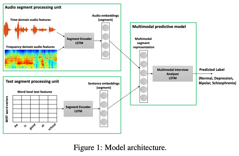
  the key insight to our model is that depending on the encoded information in textual and acoustic modalities, the relative importance of their associated learned embeddings may differ in the bimodal feature fusion layer.

  • textual feature representation layer uses 1) segment-level features extraction to learn fine-grained textual embeddings for every segment, and 2) emotion-specific representation of text segment which extracts emotion information contained in every segment. These two are then concatenated as a single text feature
  • audio feature extraction module also uses: 1) segment-level acoustic features extraction to learn audio embeddings for every segment, and 2) emotion-specific representation of audio segment

**Speech Processing Approach for Diagnosing Dementia in an Early Stage **

• Our hypothesis is that any disease that affects particular brain regions involved in speech production and processing will also leave detectable finger prints in the speech. This paper, in particular, aims to detect Alzheimer’s disease

• dataset

  • standard protocol for collecting speech samples for aphasia work is to ask volunteers to describe what they see in a picture
  • features: from speech to
    • acoustic feature extraction using pitch, energy, and voice activity detector
    • linguistic feature extraction using POS tags, syntactic complexity, LIWC, and syntactic density.
  • the pen-and-paper test for this before was the MMSE score.
    • MMSE scores greater than or equal to 24 points (out of 30) indicates a normal cognition.
    • Below this, scores can indicate severe (≤9 points), moderate (10–18 points) or mild (19–23 points) cognitive impairment

• goal, develop a system that is fully automatic (without assessing the MMSE test)

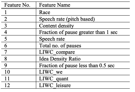
  • with MMSE, the accuracy achieved was 94.4% using only five features, one of which was the MMSE score. The five features selected (in order of importance) were MMSE score, race, fraction of pauses greater than 10sec, fraction of speech length that was pause and LIWC.

  • without MMSE, In order to achieve the 91.7% accuracy, 12 features were needed:

    

Speech Analysis: Sarcasm, Simile and Metaphor; WordsEye

$R^3$: Reverse, Retrieve, and Rank for Sarcasm Generation with Commonsense Knowledge

• generating sarcasm is challenge: there is no parallel corpus of non-sarcastic to sarcastic text

• even if we have this data, generating novel sarcasm would be issue

• approach: $R^3$ reversal, retrieve, and re-rank

  • motivating example:

    • reverse valence “Zero visibility in fog makes driving difficult” $\to$​ “Zero visibility in fog makes driving easy”
    • retrieve common sense and append: “Zero visibility in fog makes driving easy” $\to$ “Zero visibility in fog makes driving easy. It is advisable to insure your …”
    • re-rank to get more semantic incongruity: “Zero visibility in fog makes driving easy” $\to$​ “Zero visibility in fog makes driving easy. Suffered three three bones in the accident.”

  • approach:

    • reversal can be simply done with wordnet

    • retrieve common sense?

      1. use COMET which is GPT-2 tuned on ConceptNet (a knowledge graph)
      2. input words without stopwords: “zero, visibility, fogs, drive, easy”
      3. COMET output: “accident”
      4. retrieve sentences that contains accident from a database: got many
      5. re-rank by Roberta tuned on MNLI, i.e., the less it entails, the more incongruity it has = the better.

      note that this entire process is purely unsupervised = generating sarcasm without any training/parallel corpus.

  • testing: against SOTA and against human annotators

Metaphor generation: again hard since there is no parallel corpus.

• here, the proposed method is an unsupervised way to create parallel corpus

• approach

  1. first taking sentences from a poetry dataset, and then find ones that has metaphoric verbs, $v$ (have existing models to do it)
  2. pick words replacing $v$ that are consistent according to COMET’s “relates to” and is literal
  3. training: train the model to input sentence from step 2, and output step 1

Simile generation:

• before it was like changing a word to do metaphor generation. But
• approach:
  • similar to above, to use COMET to a literal version of a similie but swapping multiple words = obtain parallel corpus = train BART

Visual metaphors:

• given a text “he is like a lion on the battlefield”, how do you create an image to represent the man is fierce while being faithful in meaning
• approach: human-AI collaboration to get a dataset
  • convert the linguistic metaphor prompt to a more detailed linguistic metaphor
  • ask some human expert to make minor edits to the above
  • prompt DALLE/Stable-Diffusion
• evaluation:
  • human evaluation
  • (image, claim) entailment? visual metaphors is a bit complex for since before it was trained with literal pairs/reasoning

---

WordsEye: An Automatic Text-to-Scene Conversion System

Reading Notes for Lecture 13

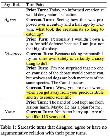
“Laughing at you or with you”: The Role of Sarcasm in Shaping the Disagreement Space

• Users often use figurative language, such as sarcasm, either as persuasive devices or to attack the opponent by an ad hominem argument. This paper then demonstrate that modeling sarcasm improves the argumentative relation classification task (agree/disagree/none) in all setups

  

• so what did they do?

  • feature based approach: extract Argument-relevant features (ArgF) such as N-gram, and Sarcasm-relevant features (SarcF) such as sarcasm markers (e.g., capitialization, quotation marks, etc.) and do logistics regression on each set.
  • NN based:
    • multitask of LSTM with sarcasm prediction + argument relation prediction
    • multitask of BERT doing the same as above
  • results, in all cases additionally including sarcasm features/modeling sarcasm gives performance improvement.

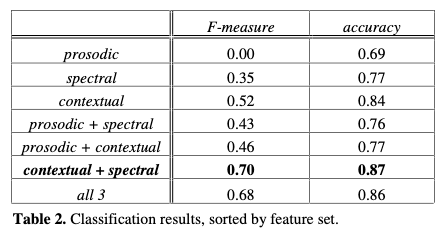
“YEAH RIGHT”: SARCASM RECOGNITION FOR SPOKEN DIALOGUE SYSTEMS

• This paper presents some experiments toward sarcasm recognition using prosodic, spectral, and contextual cues. This paper shows that spectral and contextual features can be used to detect sarcasm as well as a human annotator would, and that prosody alone is not sufficient to discern whether a speaker is being sarcastic.
• task: classify if “year right” is sarcastic or not.
• approach:
  • non-prosodic features include “whether or not tehre is laughter”, “whether the ‘year right’ is an answer or a question”, etc.
  • prosodic features: average pitch, energy, intensity, etc.
• results:
  • with human annotators trying to label them, they found it only works when context is provided: Insofar as a sarcastic tone of voice exists, a listener also relies heavily on contextual and, when available, visual information to identify sarcasm
  • experiments using decision tree classifier found that using prosody feature at all will hurt performance
  • 

“Sure, I Did The Right Thing”: A System for Sarcasm Detection in Speech

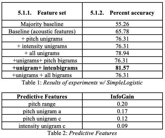
• In this paper, we present a system for automatic sarcasm detection in speech. The authors found that you can 1) use pitch and intensity contours, and 2) using a SimpleLogistic (LogitBoost) classifier to predict sarcasm with 81.57% accuracy. This result suggests that certain pitch and intensity contours are predictive of sarcastic speech.

  • so this is a counter argument of the previous paper.

• first they found that prior sarcasm related corpus is problematic, and therefore constructed their own sarcasm corpus based on “Daria”. We collected what we determined to be 75 sarcastic sentences and 75 sincere sentences – these judgments took context into consideration.

  • first they went on to let human participants rate them as the definition of “sarcasm” varies. They found that instead of a bimodal distribution, there was a trimodal distribution ni annotation:

    

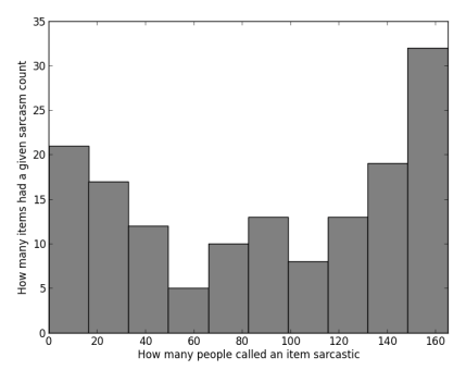
    indicating that there are also a substantial number of sentences for which participants were inconsistent.

• so how to do you model this?

  • use sentence level acoustic features such as mean pitch, pitch range, mean intensity, speaking rate, and etc

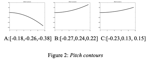
  • use word level acoustic features: prosodic contours within each word modeled by a 3 coefficient Legendre polynomial expansions, and then do some clustering + distance over all words to provide a contour over the entire sentence:

    

  • simply use Logistics regression based on the above features, and find that a (baseline is the sentence-level acoustic feature)

    

Speech Analysis: Charismatic speech

How to make charismatic speech?

• is it what you say?

• or how you say it?

• are there differences across culture?

Some experiments done and results:

• First American English Experiments: speech from democratic nomination for US president in 2004

  • found that raters have good agreement on if a speaker is “accusatory, angry, passionate, intense”, but not very good agreement on “desperate, friendly, trustworthy”
  • also tested this on arabic speakers/raters, and find strong correlation in “passionate and charismatic”

• is there any correlation between charismatic and other characteristics? Found positive correlation on:

  • enthusiastic, persuasive, not boring, and more
  • for Arabic, also found correlation on enthusiastic, persuasive, not boring

• does content matter? Measured how certain topics could correlate to charismatics

  • english: speech about healthcare, postwar Irqa, reasons for running, greating, taxes, etc.
  • arabic: skipped.

  so it definitely does matter! Additionally

  • using “our” is better than using “you”
  • lower complexity (grade-level content) is helpful (for winning elections)
  • positive emotions words: love, nice, etc.

• does speech matter? Found positive correlation on:

  • duration: longer better
  • speaking rate:
    • faster is better for english, but faster is worse for arabic
    • higher pause to word ratio is better
    • high F0 is better for both cultures
  • TOBI labels:
    • !H* and L+H* positively correlated with charisma rating for both languages (ends with a high/emphasis note = engaging)
    • L* has a negative correlation
  • ratio of repeated words is surprisingly helpful with charismatic

• interesting, when speakers rate speech which they don’t understand

  • charisma ratings is positively correlated across language even without understanding it